Patterns in Saccharomyces cerevisiae yeast colonies via magnetic resonance imaging

Abstract

We report the use of high-resolution magnetic resonance imaging methods to observe pattern formation in colonies of Saccharomyces cerevisiae. Our results indicate substantial signal loss localized in specific regions of the colony rendering useful imaging contrast. This imaging contrast is recognizable as being due to discontinuities in magnetic susceptibility (χ) between different spatial regions. At the microscopic pixel level, the local variations in the magnetic susceptibility (Δχ) induce a loss in the NMR signal, which was quantified via T₂ and T₂* maps, permitting estimation of Δχ values for different regions of the colony. Interestingly the typical petal/wrinkling patterns present in the colony have a high degree of correlation with the estimated susceptibility distribution. We conclude that the presence of magnetic susceptibility inclusions, together with their spatial arrangement within the colony, may be a potential cause of the susceptibility distribution and therefore the contrast observed on the images.

---

Insight, innovation, integration

This work presents a new method to study patterns in microorganism colonies. We applied magnetic resonance imaging methods to observe pattern formation in colonies of Saccharomyces cerevisiae. The contrast and signal efficiency allow for spatial resolution capable of differentiating the typical petal/wrinkling patterns observed in the colony that radially originate from a central hub. Interestingly, these different regions show marked signal contrast which is certainly associated with colony cell distribution and structural heterogeneity. Therefore the reported imaging method allows for one to investigate the process of yeast colony formation. Finally, the method is noninvasive and, by simply manipulating external pulse sequence parameters, the contrast can be tuned for specific regions or even completely suppressed.

1. Introduction

The microorganism Saccharomyces cerevisiae is one of the most studied yeasts. The interest on this microorganism rests on its easy handling compared to other yeasts, its use as a eukaryotic model cell, and its controllable growth.^1–4 This microorganism is largely used as an active ingredient in pharmaceutical drug formulations (probiotics) applied in the treatment of gastric-intestinal diseases.^5,6

Saccharomyces cerevisiae when growing in solid, liquid or semi-solid surfaces develop two main types of structure patterns called either colonies or biofilms. These structures consist of the growing mass of reproducing cells that spread in two or three dimensions. These structures have defined boundaries and specialized functions.^7–9 A distinction between these two structures depends upon the nature of the developing substrate. The term biofilm is utilized when describing structures formed in a natural habitat, on a substrate of complex nature and with an uncontrolled amount of nutrients. A complex structured growth is expected from a biofilm environment. Conversely, the term colony is used for a structure grown in a controlled surface with, at least, qualitative information about the content of the substrate.^10–13 Nevertheless, these terminologies are sometimes used interchangeably.^14,15 In this work, we will use the definitions above to address colony growth.

In structured colonies, the elucidation of the fundamental aspects that lead to a specific pattern is of great interest. It is known that genetic aspects and phenotype alterations, such as exposition to low levels of carbon source, nutrition levels, stiffness of the growing surface, and changes to the ambient conditions (relative humidity and temperature) can induce different kinds of colony patterns.^16–20

Pattern formation in colony growth has been studied using various imaging techniques used in biomedical sciences.^21–23 Recently, it has been shown that scattered light images of bacterial colonies could be used as a new method to identify the microorganism, given that the scattered light contains a signature of the characteristic morphologies of each microorganism. This experimental approach has been tested with success in attributing the identities of the microorganism.^24–26 Using confocal microscopy, Wilking et al. were able to show the self-formation of capillary channels in the surface of Bacillus subtilis biofilms of a wild type strain and their role in liquid transportation inside the colony.²⁷ A different approach illustrates the use of confocal microscopy in the study of biofilm architecture formation in Pseudomonas aeruginosa, revealing the contribution of exopolysaccharides in the formation of structured heterogeneous biofilm surfaces.²⁸

High field magnetic resonance imaging (MRI) provides the opportunity to improve resolution and evaluate details at the microscopic scale noninvasively. Furthermore the presence of spatial magnetic heterogeneities allows for enhanced contrast. Here, we used magnetic resonance micro-imaging (micro-MRI) to study the pattern of colonies of Saccharomyces cerevisiae growing in flat surfaces. Although our focus here is different, this imaging technique has been used before in the study of liquid flow through biofilms growing in porous materials.^29–31 Interestingly, direct imaging of the colony has not been reported. We plan here to investigate the potential of high field MRI to spatially resolving the structure of a colony where new features of biofilm structure may be detectable. The emphasis here will be on the understanding of the observed images focusing on the NMR relaxation parameters that are responsible for the contrast seen.

2. Experimental

2.1 Colony strain and growth conditions

Saccharomyces cerevisiae strain fr1972, from the probiotic Florax™ (HEBRON company), were grown in semisolid media YAPD (1% yeast extract, 2% peptone, 2% dextrose and 0.3% agar–agar). 2 mL of the semi-solid culture media YAPD were distributed into several bottom-flat glass vials with 22 mm of internal diameter. 2 μL volumes of a phosphate buffer suspension of S. cerevisiae (concentration of 10⁸ cells per mL) were gently poured into the center of the medium culture and, after drying, the vials containing the yeast were incubated at 23 °C, in a upright position, for 6 days. Controlled relative humidity conditions during incubation were obtained by placing the vials inside closed boxes containing over saturated salt solutions. To obtain the desired condition of relative humidity, RH = 32%, a CaCl₂ salt was used. The relative humidity in all boxes was monitored using hygrometers placed inside the boxes.

2.2 Micro-MRI experiments

Micro-MRI experiments were performed using VARIAN UNMRS 400 MHz (9.4 T) equipped with a microimaging probe. Two basic pulse sequences were employed: GEMS (Gradient Echo Multi Slice) and SEMS (Spin Echo Multi Slice). The pulse sequence parameters were adjusted to obtain a satisfactory signal to noise efficiency without affecting the quality of the images. To guarantee no saturation of the NMR signal, the repetition time (T_R) was set to approximately 5T₁ (T_R = 5 s). The flip angle was calibrated and adjusted to 90° in all sequences. Unless when explicitly stated, the echo times (T_E) during the experiments were 5 ms and 15 ms for the GEMS and SEMS sequences, respectively. MGEMS (Multi Gradient Echo Multi Slice) and MEMS (Multi Echo Multi Slice) were utilized when obtaining T_E variable images.

The MEMS sequence works as a CPMG sequence: there is an interval between echoes δT_E where π refocusing pulses are sandwiched with space encoding gradients. Therefore setting the interval between echoes and the number N of echoes to be acquired one will be able to register a total of N images with different echo times where, for a given N_i image, one has a T_E = N_iδT_E for the echo decay period. With this arrangement, one limits the effect of signal decay caused by diffusion to the δT_E interval. The number of echoes in the MEMS sequence was fixed to N = 64 with δT_E = 5 ms. The echo times varied then from 5 ms up to 320 ms for each image acquired in steps of 5 ms. MEMS eliminates the effects of static inhomogeneous fields whereas diffusion decay will occur only during the 5 ms intervals between echoes. For the MGEMS sequence, both diffusion decay and inhomogeneous field decay remain and increase their effects as longer T_E echoes are acquired. The data matrix was set to 256 × 256 in all images. The field of view was 25 × 25 mm, unless otherwise stated in the text, which corresponds to a resolution of ≈97 μm per pixel.

T ₂ and T₂* spatial maps are obtained by fitting, pixel by pixel, the signal decay in a series of images, MEMS and MGEMS, respectively, obtained for an interval of T_E values. The signal decay for each pixel in a sequence of images was adjusted using the equation S = S₀ exp(−T_E/T₂) (in the case of gradient echo images, T₂ should be changed for T₂*).

3. Results and discussion

3.1 Gradient and spin echo images of Saccharomyces cerevisiae colonies

The spin echo (SEMS) sequence can be used to generate density images if the repetition time is made long enough (T_R ≫ T₁), and the echo time short enough (T_E ≪ T₂), such that all hydrogen nuclear spins in the colony can be observed. Furthermore, using this sequence, the echo defocusing effect produced by inhomogeneities of the susceptibility local fields (B_loc) is reduced. Therefore the decay of the spin-echo signal with increasing values of T_E becomes sensitive primarily to the spin–spin relaxation time T₂. If the condition T_R ≫ T₁ is satisfied and T_E is varied, the sequence can be used to obtain multiple images rendering a spatial T₂ map which is sensitive to molecular mobility in different regions of the colony.^32,33

In the gradient echo (GEMS) sequence the variation in the local fields, generated by susceptibility effects, is not eliminated and increases with the echo time T_E. While the inhomogeneity of the external magnetic field (B₀) in high resolution NMR equipment can be made negligibly small, the same cannot be said about the local field variations generated by susceptibility gradients. These local field distributions are mainly generated by variations in the magnetic susceptibility (χ) of the constituents of the colony. A difference in magnetic susceptibility, Δχ, at the microscopic level (pixel dimension), will induce a phase shift Δϕ₀ = γΔBT_E, with ΔB = ΔχB₀ denoting the local field variation. This phase averaging process within the pixel is responsible for the observed signal contrast.^32,34 This contrast is particularly important at the interfaces between regions with different magnetic susceptibility distributions. Likewise in the spin echo sequence, with gradual changes in T_E, it is possible to obtain a spatial T₂* map that also includes the local field dephasing contributions due to susceptibility gradients. The separation between the T₂ and susceptibility gradient contributions from T₂* can be cumbersome but some strategies have been proposed.^35–37

Fig. 1 shows two typical images of the same colony of S. cerevisiae obtained by standard gradient echo (b) and spin echo (c) pulse sequences. Fig. 1(a) shows a coronal image slice of the colony. Highlighted on this image is the axial slice region for all the images that will be reported in this work. The colony was incubated in a semi-solid culture medium of YAPD for 6 days, at a temperature of incubation (T_i) equal to 23 °C and RH = 32%. A large difference between the contrast from the two images of the colony is apparent and some general features are worth noticing. The colony resembles a flower shape with a radial symmetry including a central hub, from where petals rise from forming surface wrinkles, at their boundaries. The choice of parameters in Fig. 1(c) corresponds to a spin density image for the selected slice of the sample (colony + culture medium).

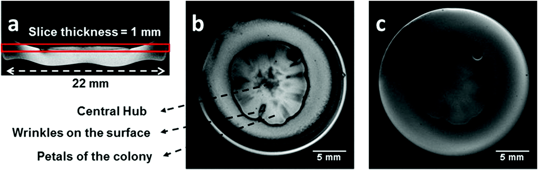Fig. 1 Images of the same colony of S. cerevisiae obtained using micro-MRI with different pulse sequences. The colony was grown for 6 days with T_i equal to 23 °C and RH = 32%. (a) Lateral view of the colony showing the selected slice position and thickness. (b) Axial image – top view of the colony – obtained using the gradient echo sequence. (c) Same slice as for (a) obtained using the spin echo sequence. In both (b) and (c), the thickness of the slice was 1 mm.

A collection of several images with gradual increases in the echo time, T_E, for both kinds of images shown in Fig. 1(b) and (c) permits the calculation of T₂* and T₂ maps, respectively. Fig. 2 shows some images obtained with this approach. Note that, the gradual loss in the intensities, as T_E is increased, is different in the two kinds of images. Whereas in the images obtained using the spin echo sequence (Fig. 2(b)) a smooth, quasi-homogeneous, decrease in the signal is observed; in the images obtained using the gradient echo sequence (Fig. 2(a)), the decrease in the signal is much more heterogeneous.

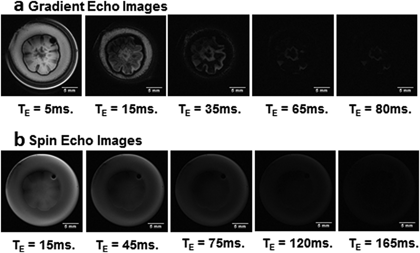Fig. 2 Images of the same colony of S. cerevisiae obtained using micro-MRI with a gradual increase in T_E. This colony was grown for 6 days with T_i equal to 23 °C and RH = 32%. (a) Image obtained using a gradient echo sequence (MGEMS) with T_R = 5 s and T_E = 5, 15, 35, 65 and 80 ms. (b) Image obtained using a spin echo sequence (MEMS) with T_R = 5 s and T_E = 15, 45, 75, 120 and 165 ms.

The reason for this difference is the contribution of the susceptibility local field generated by differences in magnetic susceptibility that are not suppressed in gradient echo pulse sequences.³⁴ Conversely, the smooth and uniform decrease in the signal intensities of the images obtained using the spin echo sequence indicates a constant distribution of hydrogen water throughout the sample. The chemical composition of both culture medium and colony is mainly water arrested in a matrix of polysaccharides and proteins with minor differences in molecular mobility.^20,38–40

The expected value for the T₂ in the agar medium should be in the range of 40–150 ms. These values are the typical values found in gels of agarose and agar, including other polysaccharides.^41,42 This low value, compared to free water (T_2water ∼ 2.72 s),³³ indicates that the water mobility in the gel matrix is restricted by its interaction with the biopolymer matrix, mainly through hydrogen bonding interaction. Throughout the colony, such mobility restriction should be similar. This explains the similar signal decay inside the colony when compared with the culture medium.

The much more significant decrease in the signal intensity in gradient echo images can be observed in the line profiles of the selected images, as shown in Fig. 3. The signal intensity along the dotted line in images (a), (b) and (c), seen in Fig. 3 yields the profiles shown in (d), (e) and (f), respectively. The profiles cover the entire structure of one petal of the colony and can be considered as representative of all petals seen in the images according to an approximate axial symmetry.

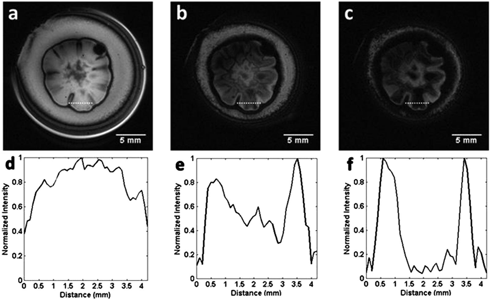Fig. 3 Gradient echo images and correlated profiles, with gradual increases in T_E. (a–c) Images obtained using a gradient echo sequence with T_E = 5 ms, 15 ms and 25 ms, respectively, for the same yeast colony. The plots in (d–f) show intensity profiles along the dotted selected line in images (a), (b) and (c) respectively.

The contrast changes drastically within the selected line profile as a function of the echo time. The signal of the region between 1.5 mm and 3.2 mm (length Δ = 1.7 mm, Fig. 3(d–f)) decreases to approximately zero, in this range of T_E variation. On the other hand, the interface of the petal with its surroundings still exhibits signal, even for T_E = 25 ms. This means that the susceptibility gradient effect inside the petals that causes the loss of the signal is more significant than in the border of the colony.

From Fig. 3(a–c), we conclude that the signal ratio between the center of the petal to the border of the petal (interface) goes from approximately 1.2, with T_E = 5 ms (Fig. 3(a)), to 0.05, with T_E = 25 ms (Fig. 3(c)). Fig. 4 shows an almost linear decrease in the signal intensity ratio for the center of the petal with respect to the border. It is worth emphasizing that the effect of the local field induced by susceptibility changes is more pronounced close to the interfaces separating regions with distinct magnetic susceptibilities being more evident as Δχ increases.³² This explains the loss of the signal, even for small T_E, for the portion of the culture medium near the boundary of the glass tube due to the air-culture medium difference of magnetic susceptibility.

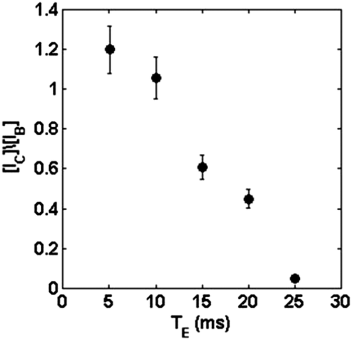Fig. 4 Evolution of the contrast between the center of the petals and the border of the colony as a function of T_E. The data were calculated by the ratio of the normalized intensity of the signal in the center of the petal in the colony (I_C) versus the normalized intensity of the border of the colony (I_B).

3.2 T ₂ and T₂* image relaxation maps of Saccharomyces cerevisiae colonies

One way of quantifying the effects discussed in the previous section is by producing T₂ and T₂* maps (see the Experimental section).⁴³

Fig. 5 shows the results obtained by this approach. The images seen in (a) and (b) of Fig. 5 represent maps of T₂* and T₂, respectively. It is important to notice that in both maps, to highlight the contrast in the images, the grey scale was inverted, so that darker regions in the image correspond to the higher values of the relaxation time. While in (b) the observed T₂ map shows a quasi-homogenous contrast in all the regions of the colony, in the T₂* map (a), the contrast is more pronounced, with a large effect of the wrinkles and boundaries of the colony.

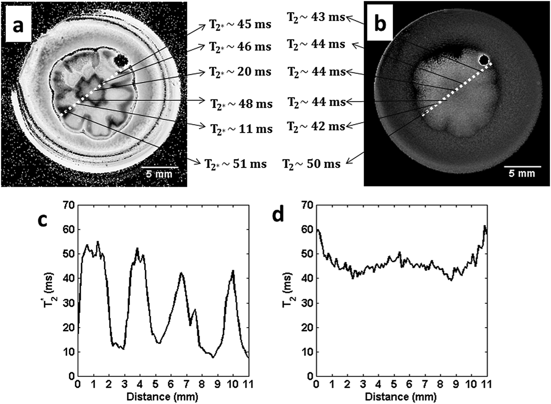Fig. 5 Maps of T₂* and T₂ of the colony of S. cerevisiae. Images (a) and (b) are the T₂* and T₂ maps, respectively, with the grey scale inverted in both images. The plots in (c) and (d) are data taken along the white dotted line of images (a) and (b), respectively.

To emphasize this visual difference, line profiles from the same region along the diameter of the colony were extracted for the two maps. Fig. 5(c) and (d) represent the T₂* and T₂ extracted from the white dotted line in (a) and (b), respectively. The line profile in (d) shows an oscillation around an average T₂ value of 46.4 ms. This oscillation around the average T₂* value (27.3 ms) is more pronounced in the line profile (c).

The large variation in T₂* values can be explained by the discontinuities of the magnetic susceptibility (χ) in the colony. The variation in the magnetic susceptibility (Δχ) introduces a factor in the signal amplitude that, in some models, scales with ∼exp(−iγgΔχB₀T_E), where γ is the constant of gyromagnetic ratio, g is the geometric factor of the magnetic susceptibility and B₀ is the applied magnetic field.^32,34 In reality, the contribution of the magnetic susceptibility to the loss of the signal is quite difficult to calculate in such a complex structure as a colony, but some simple models may be helpful.

As an illustration of the effect of susceptibility gradients, one can discuss the variation of the local magnetic field (ΔB_local) for a cylindrical symmetry inclusion. Assuming that the magnetic susceptibility inside the cylinder is constant and different from outside, the local magnetic field can be expressed, inside the cylinder, by approximately ΔB_in = gΔχB₀, where g = (3 cos² θ − 1)/6 and θ is the angle between the direction of the main magnetic field B₀ and the axis of orientation of the cylinder. On the other hand, outside the cylinder, the variation in the magnetic field induced by the difference in the magnetic susceptibility is dependent on the distance (r) from the cylinder, ΔB_out(r), and scales with ∝ΔχB₀/r².^34,44 These relations indicate that the effect of a variation in the local susceptibility has a dependence on the orientation of the structure with respect to the main magnetic field, and also on the distance (r) from the source of the magnetic susceptibility variation.

The extrapolation of the above relationships to the structure of the colony, which is much more complex than the simple case of a cylinder, allows some possible explanations for the heterogeneity in the T₂* that can be seen in the T₂* map. First, the wrinkled contour that defines the borders of the colony always appears darker than other parts, corresponding to the largest values of T₂*. Furthermore, the measured values in this region are very close to the T₂ values, as can be inferred from Fig. 5(a) and (b). If it is assumed that the relationship 1/T₂* = (1/T₂) + γΔB holds,³⁵ one can conclude that in this region (wrinkle) the local field due to susceptibility gradients is negligible, since 1/T₂* ∼ 1/T₂.

Conversely, looking to the relaxation time values found around the vicinity of the center of the petals and in the central hub of the colony, in both maps (Fig. 5(a) and (b)), and making a similar analysis, it can be observed that the ratio of these values changes by a factor of approximately 3.8 in the petals and 2.2 in the central hub. So it can be concluded that in these regions there is a signal dephasing effect induced by a change in the local magnetic field, which is stronger in the regions of the petals than in the central hub.

In fact, if we apply the above relaxation time relationship, we can roughly estimate the size of the magnetic susceptibility variation, Δχ, in these two regions. This is simply done by Δχ = ΔB/(B₀〈g〉), where ΔB = ((1/T₂*) − (1/T₂))/γ, and 〈g〉 is the geometric factor averaged over all possible values of θ in a sphere. To simplify the analysis, the geometric factor can be assumed to be equal to the cylindrical case, as discussed earlier. Therefore, the averaged value of the geometric factor can be approximated by 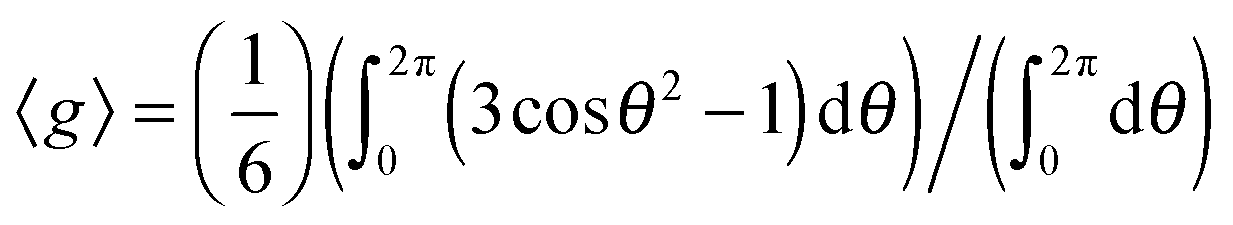. The assumption that 〈g〉 has been averaged over all possible angles in a sphere finds a reasonable justification. Around the vicinity of the petal and inside the central hub, there is not a preferential orientation of the objects with respect to the main magnetic field. In the S. cerevisiae colony the discontinuity in the magnetic susceptibility when going from one cell to another and through the interfaces and extracellular matrix induces a rapid change in χ which leads to the drop in the signal. Fig. 6 illustrates the above model to explain the variation in magnetic susceptibility.

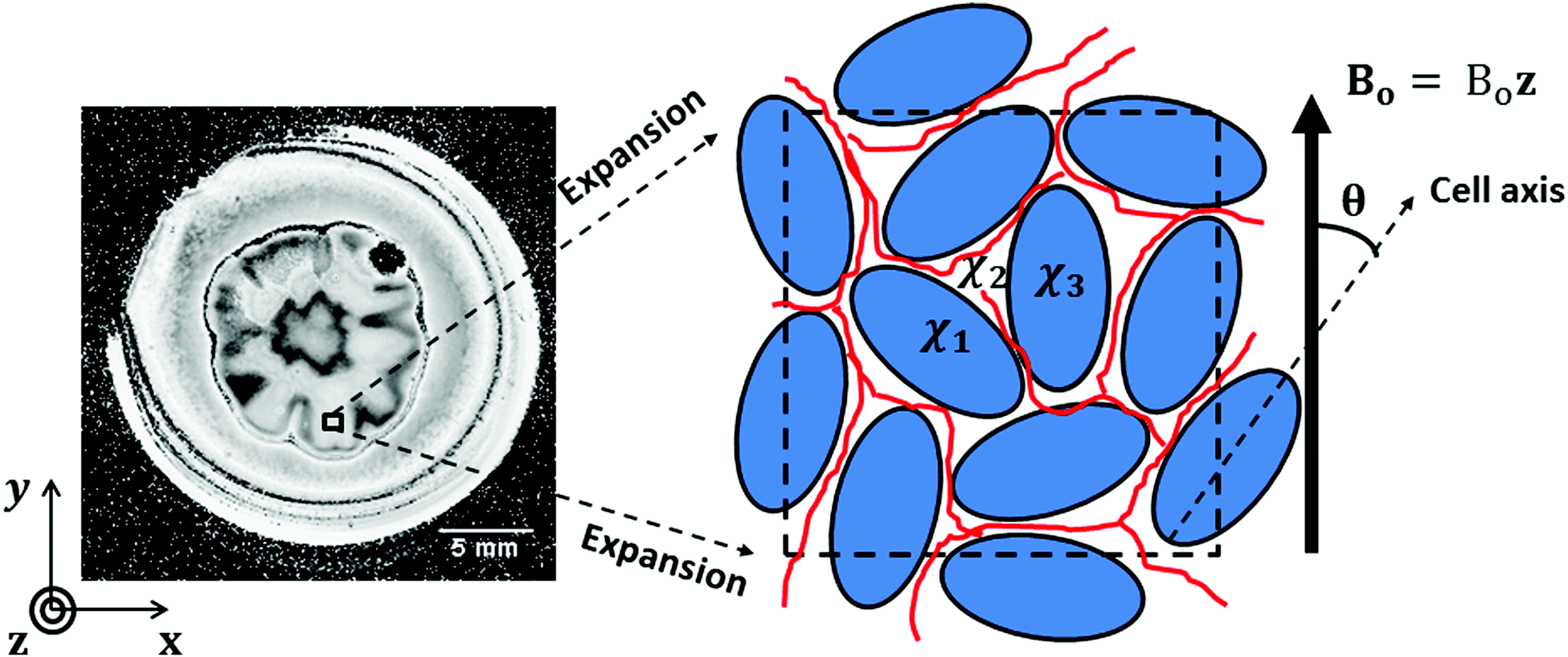Fig. 6 Schematic illustration of magnetic susceptibility variation. The ellipses represent the cells of S. cerevisiae of the selected area, showing the cell axis orientation with respect to the main magnetic field which is aligned along the z direction.

Taking the magnetic field, B₀, as equal to 9.4 × 10⁴ G, the constant of gyromagnetic ratio, γ, as 2.685 × 10⁴ G⁻¹ s⁻¹ and the values of T₂* and T₂ as 11 ms and 42 ms, respectively, for the region in the petal, and as 22 ms and 44 ms, respectively, for the region in the central hub, and calculating the value of 〈g〉, an estimate of the magnetic susceptibility variation is quite straightforward. In the region of the petal, the calculated Δχ was approximately 0.319 ppm and 0.108 ppm in the region of the central hub (in SI units).

These values are of the same order of magnitude as typical values found for biological tissue. In deoxygenated versus oxygenated blood, for instance, Δχ is found to be approximately 0.45 ppm.³⁴ In another study, the correlation between the iron content, in some parts of the human brain, and Δχ was investigated, and a value around 0.21 ppm was correlated with an iron concentration of 60 μg g⁻¹ of dry tissue.⁴⁵

Nevertheless, the susceptibility effect observed in the petals and in the central hub cannot be attributed solely to the amounts of paramagnetic cations inside the cells of S. cerevisiae that are located in these regions. As was stated in a recent paper, the content of iron, manganese and other paramagnetic species in cells of S. cerevisiae depends on the amount available in the culture medium.^46,47 However, it was demonstrated, through analysis of gradient echo MRI in human brains, that more important than the amounts of paramagnetic entities and other magnetic inclusions particles, like proteins and lipids, present in the biological system, is their spatial distribution at cellular and subcellular levels, with increasing importance of the pattern formed by the developing architecture.⁴⁸ In other words, any changes in the cultivation and growing conditions of the S. cerevisiae, with impact in the colony architecture, would lead to a different MRI imaging pattern.

Furthermore, a factor of almost 3 in ratio between the Δχ measured in the petals and in the central hub indicates that in the central hub the presence of magnetic inclusions is less pronounced. This could be explained by the known fact that in the center of the colony the rate of cell division is much slower than in the borders, due to the difficulty of the cells in that region to obtain nutrients for growth.⁴⁹ This condition will reduce the influx of driven chemical substances, from the medium to the central hub.

4. Conclusions

Images of colonies of Saccharomyces cerevisiae were obtained using high-field micro-MRI. The images exhibited contrast sensitivity due to susceptibility gradients caused by spatial magnetic heterogeneity across the structure of the colony. By changing specific NMR pulse sequence parameters an increase or suppression of contrast between the signal from different regions of the colony was monitored.

The regions of increased susceptibility coincide with the areas of specific colony regions, namely the petal structure. The increased susceptibility in these regions could be associated with cell concentration. We can also establish correlation between the reduced contrast in the central hub and the cell distribution viability in that region. This interpretation is reinforced by the work of Reynolds et al. (2008) that shows a little growth rate in the center of the colony as compared to the periphery.¹⁹

Our experimental approach opens a new way to noninvasively study patterns and self-assembly in the colonies of the microorganism by taking advantage of the spatially resolved physico-chemical sensitivity of micro-MRI. We would like to emphasize that, apart from the intrinsic structure features of the colonies, the susceptibility contrast depends both on field intensity and image resolution. Therefore this type of contrast may not be available at low magnetic fields. In the future we plan to obtain quantitative maps of paramagnetic concentration as well as diffusion and elucidate their possible role on the pattern formation contrast mechanism.

Acknowledgements

We thank Prof. Mario Engelsberg for helpful comments. This work was financially supported by the Brazilian Scientific Agency FACEPE (process number: APQ-1245-1.06/15).

References

1. H. Karathia, E. Vilaprinyo, A. Sorribas and R. Alves, PLoS One, 2011, 6(2), e16015,  DOI:10.1371/journal.pone.0016015.
2. D. Botstein, S. A. Chervitz and J. M. Cherry, Science, 1997, 277(5330), 1259–1260.
3. L. Alberghina, G. Mavelli, G. Drovandi, P. Palumbo, S. Pessina, F. Tripodi, P. Cocetti and M. Vanoni, Biotechnol. Adv., 2012, 30, 52–72.
4. G. G. Stewart, Saccharomyces cerevisiae, In Encyclopedia of Food Microbiology, ed. C. A. Batt, Academic Press, London, UK, 2nd edn, 2014, pp. 309–315.
5. D. Czerucka, T. Piche and P. Rampal, Aliment. Pharmacol. Ther., 2007, 26(6), 767–778.
6. T. Kelesidis and C. Pothoulakis, Ther. Adv. Gastroenterol., 2012, 5(2), 111–125.
7. V. Štóvíček, L. Váchová and Z. Palková, Commun. Integr. Biol., 2012, 5(2), 203–205.
8. T. B. Reynolds and G. R. Fink, Science, 2001, 291, 878–881.
9. L. Chen, J. Noorbakhsh, R. M. Adams, J. Samaniego-Evans, G. Agollah, D. Nevozhay, J. Kuzdzal-Fick, P. Mehta and G. Balázsi, PLoS Comput. Biol., 2014, 10(12), e1003979,  DOI:10.1371/journal.pcbi.1003979.
10. H. Mikkelsen, Z. Duck, K. S. Lilley and M. Welch, J. Bacteriol., 2007, 189(6), 2411–2416.
11. C. Hung, Y. Zhou, J. S. Pinkner, K. W. Dodson, J. R. Crowley, J. Heuser, M. R. Chapman, M. Hadjifrangiskou, J. P. Henderson and S. J. Hultgren, mBio, 2013, 4(5), e00645,  DOI:10.1128/mBio.00645-13.
12. R. Sidari, A. Caridi and K. S. Howell, Int. J. Food Microbiol., 2014, 189, 146–152.
13. Z. Palková, EMBO Rep., 2004, 5(5), 470–476.
14. L. Váchová, V. Štóvíček, O. Hlaváček, O. Chernyavskiy, L. Štěpánek, L. Kubínová and Z. Palková, J. Cell Biol., 2011, 194(5), 679–687.
15. V. Štóvíček, L. Váchová, M. Kuthan and Z. Palková, Fungal Genet. Biol., 2010, 47, 1012–1022.
16. J. S. Finkel and A. P. Mitchell, Nat. Rev. Microbiol., 2011, 9(2), 109–118.
17. E. A. Hope and M. J. Dunham, G3: Genes, Genomes, Genet., 2014, 4(9), 1773–1786.
18. J. A. Granek and P. M. Magwene, PLoS Genet., 2010, 6(1), e1000823,  DOI:10.1371/journal.pgen.1000823.
19. T. B. Reynolds, A. Jansen, X. Peng and G. R. Fink, Eukaryotic Cell, 2008, 7(1), 122–130.
20. J. N. Wilking, T. E. Angelini, A. Seminara, M. P. Brenner and D. A. Weitz, MRS Bull., 2011, 36, 385–391.
21. L. E. P. Dietrich, C. Okegbe, A. Price-Whelan, H. Sakhtah, R. C. Hunter and D. K. Newman, J. Bacteriol., 2013, 195, 1371–1380.
22. H. Gu, S. Hou, C. Yongyat, S. D. Tore and D. Ren, Langmuir, 2013, 29, 11145–11153.
23. Y. Chao and T. Zhang, Anal. Bioanal. Chem., 2012, 404(5), 1465–1475.
24. P. P. Banada, K. Huff, E. Bae, B. Rajwa, A. Aroonnual, B. Bayraktar, A. Adil, J. P. Robinson, E. D. Hirleman and A. K. Bhunia, Biosens. Bioelectron., 2009, 24, 1685–1692.
25. P. P. Banada, S. Guo, B. Bayraktar, E. Bae, B. Rajwa, J. P. Robinson, E. D. Hirleman and A. K. Bhunia, Biosens. Bioelectron., 2007, 22, 1664–1671.
26. E. Bae, D. Ying, D. Kramer, V. Patsekin, B. Rajwa, C. Holdman, J. Sturgis, V. J. Davisson and J. P. Robinson, J. Biol. Eng., 2012, 6, 1–12.
27. J. N. Wilking, V. Zaburdaev, M. De Volder, R. Losick, M. P. Brenner and D. A. Weitz, Proc. Natl. Acad. Sci. U. S. A., 2013, 110, 848–852.
28. M. Ritenberg, S. Nandi, S. Kolusheva, R. Dandela, M. M. Meijler and R. Jelinek, ACS Chem. Biol., 2016, 11(5), 1265–1270.
29. B. Ramanan, W. M. Holmes, W. T. Sloan and V. R. Phoenix, Curr. Microbiol., 2013, 66, 456–461.
30. B. Manz, F. Volke, D. Goll and H. Horn, Biotechnol. Bioeng., 2003, 84(4), 424–432.
31. S. J. Vogt, A. B. Sanderling, J. D. Seymour and S. L. Codd, Biotechnol. Bioeng., 2013, 110(5), 1366–1375.
32. Y. Xia, Concepts Magn. Reson., 1996, 8, 205–225.
33. P. T. Callaghan, k-Space microscopy in biology and materials science, Principles of Nuclear Magnetic Resonance Microscopy, Oxford University Press, New York, 1st edn, 1991, pp. 228–327.
34. E. M. Haacke, S. Mittal, Z. Wu, J. Neelavalli and Y. C. Cheng, Am. J. Neuroradiol., 2009, 30, 19–30.
35. G. B. Chavhan, P. S. Babyn, B. Thomas, M. M. Shroff and E. M. Haacke, Radiographics, 2009, 29(5), 1433–1449.
36. S. C. L. Deoni, B. K. Rutt and T. M. Peters, Magn. Reson. Med., 2003, 49, 515–526.
37. D. A. Yablonskiy and E. M. Haacke, Magn. Reson. Med., 1997, 37, 872–876.
38. G. S. Baillie and L. J. Douglas, J. Antimicrob. Chemother., 2000, 46, 397–403.
39. A. Beauvais, C. Loussert, M. C. Prevost, K. Verstrepen and J. P. Latgé, FEMS Yeast Res., 2009, 9, 411–419.
40. D. Romero, C. Aguilar, R. Losick and R. Kolter, Proc. Natl. Acad. Sci. U. S. A., 2010, 107, 2230–2234.
41. E. Davies, Y. Huang, J. B. Harper, J. M. Hook, D. S. Thomas, I. M. Burgar and P. J. Lillford, Int. J. Food Sci. Technol., 2010, 45, 2502–2507.
42. B. Dai and S. Matsukawa, Carbohydr. Res., 2013, 365, 38–45.
43. E. M. Haacke, R. W. Brown, M. R. Thompson and R. Venkatesan, Magnetic Resonance Imaging: Physical Principles and Sequence Design, John Wiley & Sons Inc, New York, 1st edn, 1999, pp. 111–138.
44. J. F. Schenck, Med. Phys., 1996, 23(6), 815–850.
45. E. M. Haacke, M. Ayaz, A. Khan, E. S. Manova, B. Krishnamurthy, L. Gollapalli, C. Ciulla, I. Kim, F. Petersen and W. Kirsch, J. Magn. Reson. Imaging, 2007, 26, 256–264.
46. G. P. Holmes-Hapton, N. D. Jhurry, S. P. McCormick and P. A. Lindahl, Biochemistry, 2013, 52, 105–114.
47. M. S. Cyert and C. C. Philpott, Genetics, 2013, 193(3), 677–713.
48. X. He and D. A. Yablonskiy, Proc. Natl. Acad. Sci. U. S. A., 2009, 106(32), 13558–13563.
49. M. Varon and M. Choder, J. Bacteriol., 2000, 182(13), 3877–3880.

---