
From millimetres to metres: the critical role of current density distributions in photo-electrochemical reactor design†‡
A.
Hankin
*,
F. E.
Bedoya-Lora
,
C. K.
Ong§
,
J. C.
Alexander¶
,
F.
Petter||
and
G. H.
Kelsall
Department of Chemical Engineering, Imperial College London, London, SW7 2AZ, UK. E-mail: anna.hankin@imperial.ac.uk
First published on 21st December 2016
Abstract
0.1 × 0.1 m2 tin-doped hematite photo-anodes were fabricated on titanium substrates by spray pyrolysis and deployed in a photo-electrochemical reactor for photo-assisted splitting of water into hydrogen and oxygen. Hitherto, photo-electrochemical research focussed largely on the fabrication, properties and behaviour of photo-electrodes, whereas both experimental and modelling results reported here address reactor scale-up issues of minimising inhomogeneities in spatial distributions of potentials, current densities and the resultant hydrogen evolution rates. Such information is essential for optimising the design and photon energy-to-hydrogen conversion efficiencies of photo-electrochemical reactors to progress their industrial deployment. The 2D and 3D reactor models presented here are coupled with a modified micro-kinetic model of oxygen evolution on hematite thin films both in the dark and when illuminated. For the first time, such a model is applied to a scaled-up photo-electrochemical reactor and validated against experimental data.
Broader contextThe abundance of solar energy on Earth and the natural photosynthesis in plants has motivated extensive worldwide research into photon capture by synthetic materials and conversion into storable fuels in a process broadly termed ‘artificial photosynthesis’. This remains focused largely on the development of materials for solar fuel production that are: (i) efficient in converting photons to chemical product(s), (ii) inexpensive to fabricate and (iii) robust. The ultimate objective is to identify the best performing materials for integration in photo-electrochemical systems. However, despite substantial progress in material development, the question ‘What might an industrial scale photo-electrochemical reactor system ultimately look like?’ still remains unanswered. This will remain so until scalable reactor demonstration units are modelled, designed, fabricated, and their performance, durability and cost assessed. Upon scale-up, several effects, often negligible at laboratory scale, become important and may limit device performance. Current density distribution is one of these effects that needs to be addressed and understood for successful reactor design and scale-up. |
Introduction
The long awaited industrial deployment of photo-electrochemical systems for hydrogen production via water splitting still necessitates considerable progress to be made in the development and operation of scalable demonstration units, coupled with numerical models that describe their performance and guide further design optimisation.The vast body of experimental work carried out to date worldwide has largely been limited to small-scale laboratory studies, focusing on the production and characterisation of potential photo-electrode materials. However, encouraging reports of experimental work in scaled systems are beginning to emerge. For the time being, we refer to ‘scaled’ systems as those incorporating photo-electrodes with lengths of 0.1 m or greater. For example, the performance of a reactor, designed to accommodate 0.1 × 0.1 m2 electrodes, during photo-assisted electrolysis has been reported by Lopes et al.1 A wide range of considerations, such as the transparency or otherwise of the photo-electrode substrate, electrode orientation within the reactor, reactor illumination, the requirement for a membrane/diaphragm for product separation, compatibility of reactor materials with the electrolyte, electrolyte flow and reactor component costs were addressed in the design of the device. More recently, a reactor with multiple pairs of series-connected a-Si:H/μc-Si:H tandem solar cells that were fully integrated inside the device and connected with nickel foam anodes and cathodes has been developed and demonstrated a solar to hydrogen (STH) conversion efficiency of 3.9% on an active area of 52.8 cm2 during solely solar-driven photo-electrolysis under 1 Sun.2 Another photo-electrochemical reactor, with electrode lengths of order 0.2 m, coupled to a novel light distribution system is currently under development.3
Modelling of photo-electrochemical processes has been a topic of more intensive research. For example, 1-D kinetic models and transport processes in photo-electrochemical systems have been studied extensively by Berger et al.4,5 Primary current and potential distributions, as well as cell resistance, have also been investigated in 2-D for reactors containing slotted semiconductor photo-electrodes by Orazem et al.6,7 However, such models are applicable to material and kinetic studies on the laboratory scale only. Haussener et al.8 developed a detailed 2-D model for determining the effects of different geometrical configurations on current density and overpotential distributions, ohmic losses, H2–O2 cross-over losses and hydrogen yield in an electrolyser operating at 200 A m−2; kinetic models applicable exclusively to metal|electrolyte interfaces were used. Subsequently, the model was extended to dual-absorber tandem cells and incorporated the semiconductor physics of the constituent materials.9 The model was used to determine the solar to hydrogen conversion efficiency as a function of the electrode characteristic length and other geometric parameters within the reactor. A more recent publication addressed additional limitations imposed on photo-electrochemical reactor performance by the photon flux, band gap and other photo-electrode parameters.10 However, there has been a lack of analyses of current and overpotential distributions along photo-electrodes in 2-D and 3-D and there is still a paucity of an experimentally validated comprehensive model that could be used for designing scaled-up systems.
In this work, we present a model describing experimental data from photo-assisted electrolysis in a photo-electrochemical reactor utilising 0.1 × 0.1 m2 electrodes (hematite photo-anode and platinised titanium cathode) of various geometries and in various geometric configurations; our experimental data corroborated the numerical model predictions in COMSOL Multiphysics 4.4. The model was developed to aid the understanding of the impact of geometric effects on current and overpotential distributions at electrode surfaces and to guide reactor design. It incorporated parameters characterising both the semiconductor and the semiconductor|electrolyte interface that were determined from our own experimental data.
Synthetic hematite, the photo-absorber and photo-anode in our study, has been subject to considerable research as a photo-anode for solar water splitting. Theoretically, its band gap of 1.9–2.2 eV11 enables it to absorb up to 37–30% of solar photons, as determined by integrating the AM 1.5 solar irradiance spectrum (ASTM G173-03 Reference Spectra12) with respect to wavelength, λ, for λ ≤ λband![[thin space (1/6-em)]](https://www.rsc.org/images/entities/char_2009.gif) gap. However, the low conductivity of hematite, even when doped, requires a conductive substrate to serve as current feeder. Typically, for use in small scale reactors, hematite films are deposited onto glass substrates coated with a thin layer of conductive fluorine-doped tin oxide (FTO). However, the manufacturer-specified sheet resistivity of 0.2–1.5 Ω cm2 (Sigma Aldrich) renders this substrate unsuitable for scale-up.13 Hence, Ti|Fe2O3 photo-anodes14 were developed for deployment in alkaline aqueous electrolytes; this was motivated by the high conductivity of titanium,15 as well as its chemical stability in such media. The formation of a TiO2 inter-layer between Ti and Fe2O3 during the fabrication process was shown not to be seriously disadvantageous, provided the TiO2 thickness does not exceed several nanometres.14 However, the lack of transparency of a comparatively thick metallic substrate limits the photo-electrode configuration geometries by which photon fluxes can be absorbed.
gap. However, the low conductivity of hematite, even when doped, requires a conductive substrate to serve as current feeder. Typically, for use in small scale reactors, hematite films are deposited onto glass substrates coated with a thin layer of conductive fluorine-doped tin oxide (FTO). However, the manufacturer-specified sheet resistivity of 0.2–1.5 Ω cm2 (Sigma Aldrich) renders this substrate unsuitable for scale-up.13 Hence, Ti|Fe2O3 photo-anodes14 were developed for deployment in alkaline aqueous electrolytes; this was motivated by the high conductivity of titanium,15 as well as its chemical stability in such media. The formation of a TiO2 inter-layer between Ti and Fe2O3 during the fabrication process was shown not to be seriously disadvantageous, provided the TiO2 thickness does not exceed several nanometres.14 However, the lack of transparency of a comparatively thick metallic substrate limits the photo-electrode configuration geometries by which photon fluxes can be absorbed.
Below, we report the experimental performance of 0.1 × 0.1 m2 Ti|SnIV–Fe2O3 photo-anodes in 1 M NaOH (and in some cases in 0.1 M NaOH) solution in two possible irradiation configurations:
(a) directly illuminated photo-anode surface facing away from the counter electrode;
(b) photo-anode surface facing towards the counter electrode mesh, which was interposed between the photo-anode and the light source.
In both cases, the reverse sides of the Ti substrates were painted with an inert (acrylic) lacquer.
The two configurations are illustrated schematically in Fig. 1(a) and (b), respectively; both configurations have advantages and disadvantages. In Fig. 1(a), the surface of the photo-electrode is illuminated directly, with some degree of attenuation of the photons with λ ≤ λbandgap by the quartz window and the electrolyte; however, with this geometry, the ionic current is forced to flow around the photo-electrode so is non-uniformly distributed, on scale-up leading to increasing undesirable inhomogeneities in the reaction rate at the photo-electrode surface. In Fig. 1(b), the illuminated photo-anode surface faces the cathode, leading to a more uniform ionic current density distribution; however, the presence of the mesh cathode, a larger body of electrolyte populated by (reflective) bubbles and, potentially, an ion permeable membrane in the pathway of the light, would lead to a significant attenuation of the incoming photon flux.
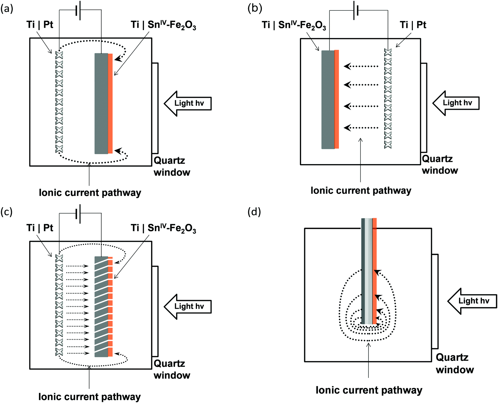 | ||
| Fig. 1 Electrode geometries and configurations investigated experimentally and/or computationally using finite element analysis in a photo-electrochemical reactor: (a) directly illuminated photo-anode surface (hematite film on a Ti foil substrate) facing away from counter electrode; (b) photo-anode surface facing towards the counter electrode mesh, which is interposed between the photo-anode and light source; (c) directly illuminated photo-anode surface (hematite film on a perforated Ti foil substrate) facing away from counter electrode; (d) directly illuminated hematite film, which is a part of a wireless ‘photo-bipole’ type electrode assembly. The current paths of OH− anions, corresponding to each scenario, are shown with dotted arrows. The photo-inactive sides of the photo-anodes were covered with insulating varnish, so were not electrochemically active. | ||
Fig. 1(c) shows a potential solution to the problem of macroscopically inhomogeneous ionic current distribution in Fig. 1(a): we propose the use of a titanium substrate, perforated in order to homogenise ionic current distributions. The perforations are made at an angle <90° to the surface in order to maximise the capture of photons.
Experimental measurements of current as a function of applied photo-anode potential obtained with the systems depicted in Fig. 1(a)–(c) are presented. Furthermore, the performances of systems (a) and (c) are compared using finite element analysis (COMSOL Multiphysics 4.4) in order to assess the effectiveness of the perforations in improving the average photocurrent density at the hematite surface in 1 M and 0.1 M NaOH solutions.
Finally, we used finite element analysis to model a wireless ‘photo-bipole’ geometry in 2-D, Fig. 1(d),16–18 in order to investigate the limitations imposed on the performance of such photo-electrochemical reactors.
The model developed for the determination of potential and current density distributions in a photo-electrochemical reactor in both 2-D and 3-D incorporated:
(1) Bulk photo-anode properties, including band gap, conductivity, dielectric constant, absorption coefficient and charge carrier density and bulk cathode properties, including the conductivity;
(2) Micro-kinetics of O2 evolution at the Ti|SnIV–Fe2O3 interface with 1 M NaOH electrolyte, based on the incident photon flux, flat band potential, charge carrier density, absorption coefficient, absorber thickness and charge separation efficiencies;
(3) Micro-kinetics of H2 evolution at the Ti|Pt cathode surface in 1 M NaOH solution;
(4) Different photo-anode geometries, including solid and perforated electrodes;
(5) Different electrode configurations, including wired and ‘wireless’ geometries.
Experimental
Photo-anode fabrication
Photo-anode electrodes were fabricated in two sizes:• 0.01 × 0.06 m2 electrodes for the purpose of determining film thickness, the flat band potential and the micro-kinetics of O2 evolution (photocurrent and dark current as a function of applied potential); the parameters determined at this scale were incorporated subsequently into the photo-electrochemical reactor model in COMSOL Multiphysics 4.4;
• 0.1 × 0.1 m2 electrodes for deployment in different configurations in a scaled-up photo-electrochemical reactor. These electrodes were produced on substrates both of Ti foil (0.74 mm thick, Alfa Aesar) and perforated Ti sheet (1 mm thick, titanium grade 2 with approximate perforation dimensions: 3 mm (L) × 1.5 mm (W), repeated every 5.8 mm horizontally and 2 mm vertically, The Expanded Metal Company), shown in Fig. 2.
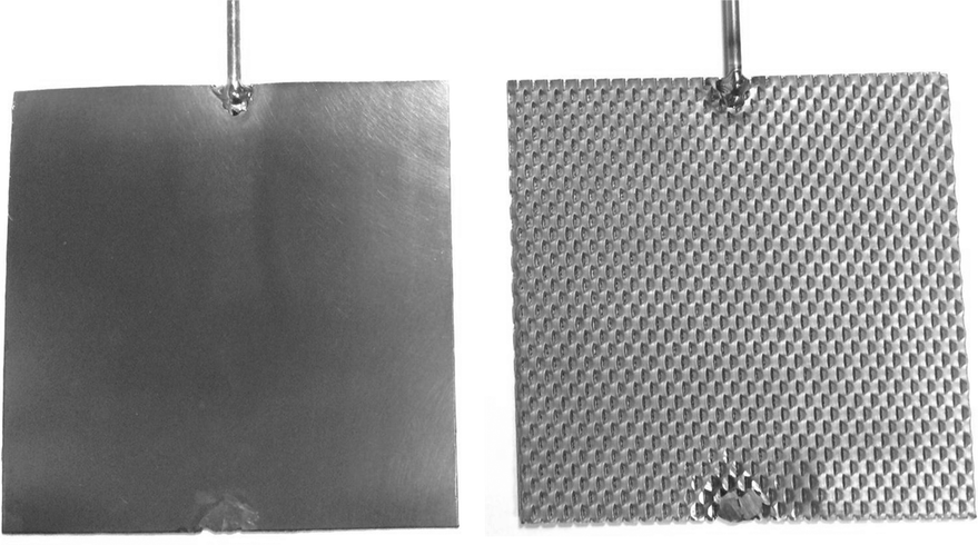 | ||
| Fig. 2 Solid and perforated 0.1 × 0.1 m2 Ti substrates employed in the scaled-up photo-electrochemical reactor (image shows substrates prior to the deposition of Fe2O3 films). Electronic contacts, made by welding, are also visible. | ||
For both electrode sizes, the tin-doped iron oxide films were deposited by spray pyrolysis.14 Prior to the deposition, the Ti foil substrates were polished using alumina powder on an automated polishing machine (Buehler), degreased with acetone, ultrasonicated, soaked in 0.5 M oxalic acid to dissolve air-formed titanium oxide and, finally, washed in de-ionised water.
The precursor solution for spray pyrolysis comprised 0.1 M FeCl3 (Sigma Aldrich, UK) and 6 × 10⁻⁴ M SnCl4 (Sigma Aldrich, UK) dissolved in ethanol absolute (AnalaRNormapur, VWR BDH Prolabo). A quartz nebuliser (Meinhard, US), which acted as the spray nozzle, was attached onto a CNC machine (Heiz T-720, Germany) and was maintained at a height of 150 mm above the surface of the substrate. The movement of the CNC was software-automated (WinPC-NC CNC Software, BobCad-CAM, USA) to facilitate the formation of homogeneous coatings. The FeIII precursor was delivered to the nebuliser by a syringe pump at 2 cm3 min−1; pressurised air was supplied at 345 kPa. During the spray pyrolysis process the substrates were maintained at 480 °C with the use of a hotplate.
Forty passes of the nebuliser over the heated substrate generated hematite coatings of 47 ± 6 nm in thickness, which was measured using a stylus profilometer (TencorAlphastep 200 Automatic Step Profiler).
Electronic contact to the electrodes was made externally with the aid of titanium rods (2 mm diameter, Alfa Aesar), pre-welded to the edges of the Ti foil substrates, as shown in Fig. 2.
To minimise dark current contributions to photocurrent densities from areas of the electrodes that were exposed to electrolyte but not radiation, such areas were coated in electrochemically inert, insulating acrylic lacquer (RS components).
Photo-anode characterisation
Unless specified otherwise, electrochemical measurements were performed in 1 M NaOH solution (pH measured ca. 13.7 and temperature 25(±2) °C) at Ti|SnIV–Fe2O3 working electrodes, with a Ti|Pt mesh (circa 56% open area, The Expanded Metal Company, UK) counter electrode and a HgO|Hg reference electrode (0.109 V vs. SHE) using a potentiostat/galvanostat (Autolab PGSTAT 30 + Frequency Response Analysis module, Eco Chemie, Netherlands). All electrode potentials are reported relative to the standard hydrogen electrode (SHE) in the results. Electrolyte conductivity was measured with a conductivity meter (Hach Lange).Photo-electrochemical characterisation of the 0.01 × 0.06 m2 photo-electrodes (exposed area of 0.003 × 0.006 m2) was performed in a 60 cm3 photo-electrochemical reactor (PVC body with a single quartz aperture). Photocurrents at these electrodes were recorded as a function of potential, applied at a scan rate of 10 mV s−1 from 0 to 1.4 V (SHE), under illumination from a 300 W Xe arc lamp (LOT-Oriel). The total power density after concentration of light with Fresnel lenses was 5600 W m−2, measured with a spectrometer (Stellarnet, UV-Vis spectrometer, BLK-CXR); the irradiance spectrum is shown in Fig. 1S in the ESI.‡ Light attenuation by the quartz window in the reactor and the NaOH electrolyte were also measured using the spectrometer in order to correct the illumination intensity incident on the hematite surface. Finally, the extent of photon absorption by the hematite film itself was measured for a SnIV–Fe2O3 sample deposited on fused silica. The absorption spectrum of the film was further used to determine the band gap of the material, which was 2.16 eV (575 nm).
Photo-electrochemical impedance spectroscopy (PEIS) using the lamp described above was used to determine electron–hole recombination efficiencies and interfacial capacitance as a function of applied electrode potential.19 Each applied potential was perturbed sinusoidally by ±10 mV (p–p) at frequencies in the range 10−1–105 Hz and the resultant impedance was measured. An equivalent electrical circuit with two time constants was used to fit experimental data. The recombination and electron transfer resistances were used to estimate the charge transfer efficiencies. Interfacial capacitance values were used to generate Mott–Schottky plots, from which the flat band potential and the electron donor density of the SnIV–Fe2O3 films were determined. Details of the calculations are presented in the ESI.‡
Photo-electrochemical characterisation of 0.1 × 0.1 m2 electrodes in the configurations shown in Fig. 1(a)–(c) was performed in a 1 dm3 photo-electrochemical reactor, under illumination from a solar simulator (Sun2000, Abet Technologies) with a 550 W Xe arc lamp; the irradiance spectrum is shown in Fig. 2S in the ESI.‡ The photo-anodes and the 0.1 × 0.1 m2 Ti Pt mesh cathode (open area circa 56%) were tested in 1 M and 0.1 M NaOH electrolytes. In addition to electrode characterisation by voltammetry, the reactor was operated in a two-electrode arrangement under a constant applied cell bias of 1.6 V for 24 hours, during which the cell current, electrolyte temperatures and evolved H2 and O2 volumes were recorded. Performance was thus assessed with both planar and perforated electrodes, as well as with 1 M and 0.1 M NaOH electrolytes. During these experiments, the anolyte and catholyte were separated by a cation-permeable membrane (Nafion 424, DuPont Inc.) in order to minimise product cross-over; gas flow rates were monitored with gas flow meters (MilliGascounter MGC-1, Ritter, Germany).
A custom-made HgO|Hg reference electrode was introduced into the anode compartment in both reactors to enable the control of the photo-anode potential.
Modelling
COMSOL Multiphysics 4.4 with a Batteries and Fuel Cells module and LiveLink for MATLAB was used to run models using the finite element method. A stationary non-linear solver and a relative tolerance for convergence criteria of 0.001 were used in all models; the suitability of this convergence criterion is demonstrated in a convergence study in the ESI.‡ A predefined ‘fine’ mesh with a maximum element size of 0.014 m and a minimum of 0.00175 m was used for the 3-D photo-electrochemical reactor model (0.1 × 0.1 m2). The suitability of this choice of mesh is demonstrated in the ESI.‡ A custom mesh with a maximum size element of 0.005 m and minimum size of 10−7 was used for the 2-D model.Fig. 3 shows a schematic view and positions of the 0.1 m × 0.1 m electrodes, separated by 0.03 m of electrolyte, in the 3-D photo-electrochemical reactor model. Due to the high ionic strength of the 0.1–1 M NaOH electrolyte employed in the experiments, the electrolyte was modelled as a homogeneous continuous medium. Electrode potentials were applied at the top of the electrical contacts: the cathode potential was fixed at zero and the anode potential was varied relative to a reference electrode (SHE), positioned as shown in Fig. 3.
 | ||
| Fig. 3 Isometric view of the reactor showing relative positions of the working (Ti|SnIV–Fe2O3 photo-anode), counter (Ti|Pt) and reference (SHE) electrodes as well as the kinetic models applied at each electrode|solution interface. | ||
 | (1) |
 | (2) |
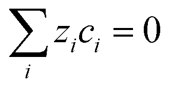 | (3) |
| ∇2ϕ = 0 | (4) |
 | (5) |
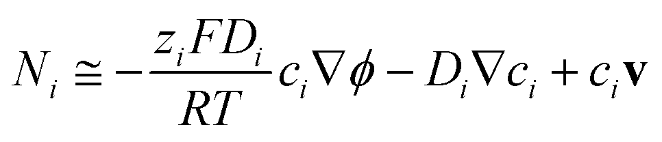
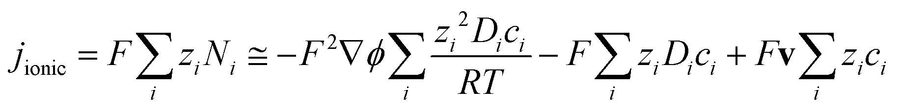
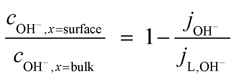
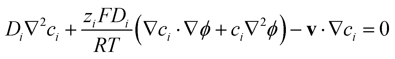
However, such high pHs may be undesirable, as they correspond to conditions in which Fe2O3 and quartz windows are predicted20 to dissolve to some extent, as are SnIV/SnII dopants, and atmospheric CO2 gas may also dissolve in electrolyte solutions unless precluded by judicious design. However, decreasing solution pHs to 10, for example, to mitigate these effects would result in concentration gradients due to depletion of OH− ions by oxygen evolution reaction at photo-anode surfaces, causing violation of assumptions for eqn (4). Under those conditions, a more complex eqn (6) would the need to be solved, allowing both for concentration and potential gradients, as in a future publication. In the steady state (∂ci/∂t = −∇·Ni = 0), eqn (1) results in:
 | (6) |
For the condition of (infinitely) dilute solutions, ionic conductivities are predicted to be linearly dependent on concentration, according to:
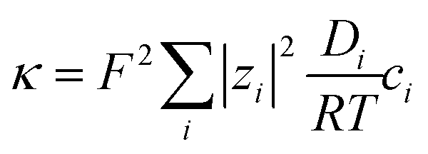 | (7) |
 | (8) |
| UH2O/H2(SHE)/V = −0.0592 pH − 0.0296logpH2 | (9) |
 | (10) |
 | (11) |
 | (12) |
 | (13) |
A further correction is introduced to account for the extent of the absorption of incident radiation by a thin film semiconductor. The absorption by a material with absorption coefficient αλ and thickness x is computed using the Beer–Lambert law:
| Ix,λ = I0,λexp(−αλx) | (14) |
 | (15) |
 | (16) |
| janode,dark ≈ j0,anodeexp(βaηanode) | (17) |
| UO2/H2O(SHE)/V = 1.23 − 0.0592 pH + 0.0148logpO2 | (18) |
| janode,total = jphoto + janode,dark | (19) |
Summary of model assumptions
• Electrochemical reactions were the oxidation and reduction of water at the photo-anode and cathode, respectively;• Charge conservation in the liquid electrolyte phase, which was modelled as a homogeneous continuous medium (i.e. concentration gradients were negligible, as were effects of any gas bubbles generated);
• Photocurrent densities were modelled using a modified Gärtner–Butler eqn (16);
• Photocurrent densities were limited by the incident photon flux and by the potential-dependent charge carrier recombination kinetics;
• Butler–Volmer kinetics were assumed for the cathodic and anodic (dark) currents;
• The condition of ∇ci = 0 was assumed for the electrolyte;
• Temperature effects were negligible for the conditions used; parameter values quoted here were determined at room temperature.
Results and discussion
Photo-electrochemical characterisation of hematite
 | ||
| Fig. 4 Oxygen evolution kinetics at a 0.01 × 0.06 m2 Ti|SnIV–Fe2O3 anode in the dark and under illumination in 1 M NaOH solution recorded at a potential scan rate 10 mV s−1; arrows indicate the direction of the potential sweep. The dotted line shows exclusively the photocurrent density, computed by subtracting the dark current density from that recorded in light. Inset shows a magnified data range. | ||
A shift of −0.6 V in the potential was observed for the oxygen evolution onset on hematite under illumination relative to the behaviour under dark conditions. The photocurrent generated by reaction (20) reached a plateau of circa 25 A m−2 (1.9 × 10⁻² A W−1), prior to the onset of dark current from reaction (21) at 0.8 V (SHE).
| 4OH− + 4h+ → O2 + 2H2O | (20) |
| 4OH− → O2 + 2H2O + 4e− | (21) |
 | ||
Fig. 5 (a) Nyquist and (b) Bode-phase plots characterising the SnIV–Fe2O3|1 M NaOH interface (0.01 × 0.06 m2 electrodes) at 0.57, 0.67 and 0.77 V (SHE) under illumination from a Xe arc lamp. Experimental (●) and modelled (![[dash dash, graph caption]](https://www.rsc.org/images/entities/char_e091.gif) ) data is presented, with the equivalent circuit shown in the inset. ) data is presented, with the equivalent circuit shown in the inset. | ||
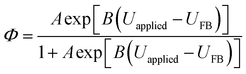
The resistances obtained using the equivalent circuit were used to compute the efficiency of interfacial electron transfer in eqn (12), according to:19
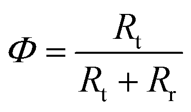 | (22) |
 | (23) |
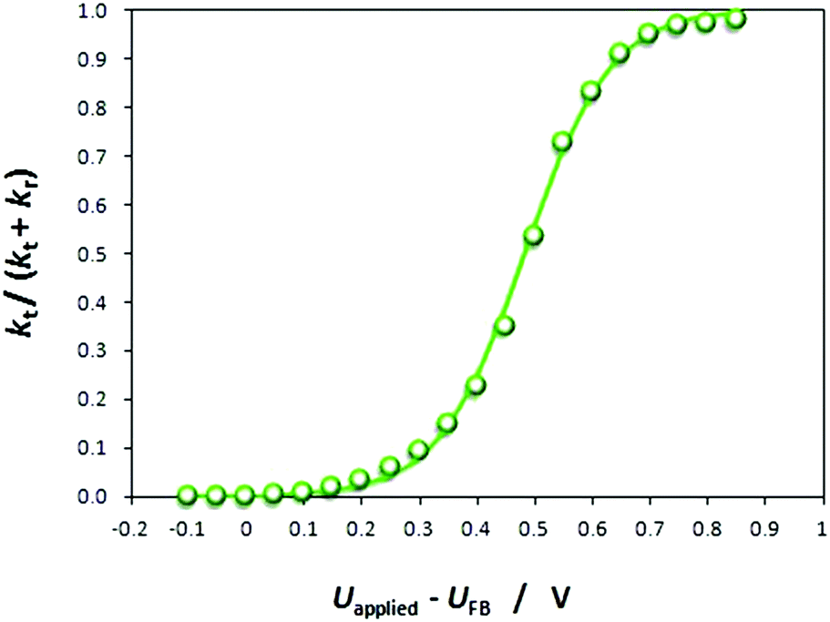 | ||
| Fig. 6 Effect of band bending (Uapplied − UFB) on interfacial transfer efficiencies for 0.01 × 0.06 m2 Ti|SnIV–Fe2O3 under illumination from a Xe arc lamp. Line shows the fit to the data obtained by non-linear regression. | ||
|electrolyte interface:25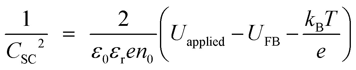 | (24) |
 | ||
| Fig. 7 Mott–Schottky plot obtained from PEIS measurements on a 0.01 × 0.06 m2 Ti|SnIV–Fe2O3 electrode in 1 M NaOH electrolyte. | ||
C SC were extracted from the constant phase elements corresponding to the high frequency semicircles, which were computed during the fitting of aforementioned equivalent circuit to experimental data according to:
| CSC = Y0,t1/nRt(1−n)/n | (25) |
U FB is determined from the intercept of the linear portion of the Mott–Schottky plot with the potential axis. For four samples, UFB (SHE) was computed to be +0.16 (±0.022) V, in agreement with predictions.26
 | ||
| Fig. 8 Predicted effects of electrode potential on photocurrent densities at a hematite|1 M NaOH interface according to the Gärtner–Butler equation and that allowing for recombination kinetics, determined from experimental electrochemical impedance data and described by eqn (10), (13), (15) and (16). | ||
| Parameter | Symbol | Value | Unit | Ref. |
|---|---|---|---|---|
| Electronic charge | e | 1.60 × 10⁻¹⁹ | A s | 30 |
| Hematite film thickness | x | 4.7 × 10⁻⁸ | m | This work |
| Band gap | E G | 2.16 | eV | This work |
| Un-attenuated light intensity (λ < 575 nm) | I | 3.57 × 10²¹ | m−2 s−1 | This work |
| Un-attenuated power density (λ < 575 nm) | P | 1.33 × 10³ | W m−2 | This work |
| Spectrally resolved product of light intensity and absorption coefficient | ∑I0,λ·αλ | 2.53 × 1029 | m−3 s−1 | This work |
| Spectrally resolved product of light intensity and absorption coefficient (corrected for attenuation by quartz and electrolyte) | ∑(I0 − Ix)λ·αλ | 1.53 × 1029 | m−3 s−1 | This work |
| Maximum photocurrent ((I0 − Ix) × e) | j photo,max | 248 | A m−2 | This work |
| A (coefficient in eqn (23)) | A | 2.61(±0.996) × 10−3 | 1 | This work |
| B (coefficient in eqn (23)) | B | 13.3(±0.972) | V−1 | This work |
| Permittivity of free space | ε 0 | 8.85 × 10⁻¹² | A s V−1 m−1 | 30 |
| Relative permittivity of hematite | ε r | 38.2(±0.463) | 1 | This work |
| Flat band potential | U FB | +0.16(±0.022) | V (SHE) | This work |
| Charge carrier density | n 0 | 2.73(±0.398) × 1027 | m−3 | This work |
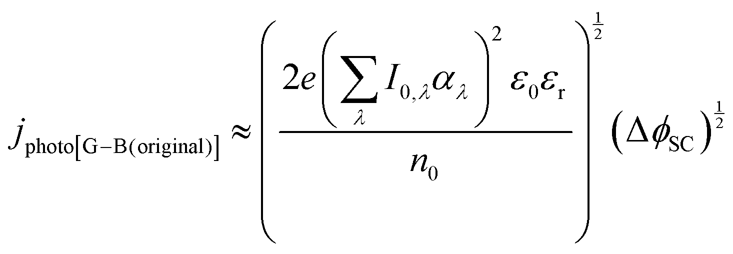
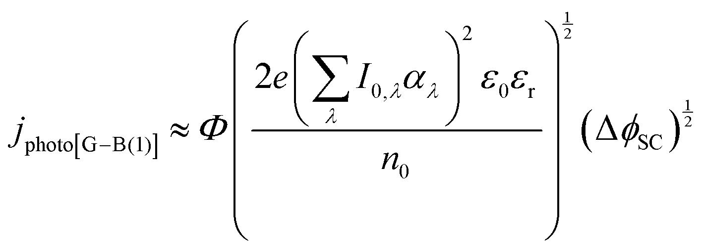
It was evident that the process of recombination considerably altered the current densities predicted by the original Gärtner–Butler equation. However, this correction alone, embodied in jphoto[G–B(1)], is not sufficient. To further improve the prediction, corrections for the attenuation of incident light by the quartz window of the reactor, the NaOH electrolyte and only partial absorption of the incident light by the thin hematite film were made in jphoto[G–B(2)]. Finally, it is important to correct the photocurrent density, predicted by jphoto[G–B(original)] to increase indefinitely with (ΔϕSC)1/2, by the limiting photocurrent density, corresponding to the incident flux for λ < λmax at a quantum yield of unity in jphoto[G–B(3)].
Fig. 9 shows the agreement between the photocurrent density predicted by jphoto[G–B(3)] using parameters in Table 1 and experimental data obtained on four SnIV–Fe2O3 samples.
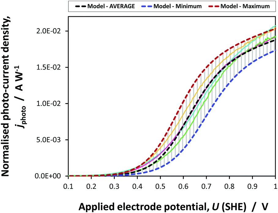 | ||
| Fig. 9 Average, maximum and minimum photocurrent densities predicted by jphoto[G–B(3)] using parameters in Table 1 and experimental data obtained on four 0.01 × 0.06 m2 SnIV–Fe2O3 samples. | ||
The prediction was made using the average values of parameters determined in this study. Error boundaries are shown by the maximum and minimum photocurrents predicted by the errors associated with n0, UFB, εr and coefficients A and B in eqn (23). The experimental data obtained on four samples falls within the error boundaries. The photocurrent densities have been normalised with respect to the incident power density to allow for the difference in intensities under which the samples were characterised. This kinetic model of the photo-anode was employed in the 2D and 3D simulations of the performance of the photo-electrochemical reactor incorporating 0.1 × 0.1 m2 electrodes.
Reactor operation with different electrode configurations
The 0.1 × 0.1 m2 photo-anodes were irradiated with light emitted by a 550 W Xe lamp in the solar simulator and reflected by a mirror.In the first instance, we conducted an experimental comparison of the currents generated at 0.1 × 0.1 m2 hematite photo-electrodes as a function of applied potential, when arranged according to the schematics in Fig. 1(a) and (b). Fig. 10 shows a comparison between front-side illumination of the 0.1 × 0.1 m2 photo-anode when positioned in front of and behind the Ti|Pt cathode mesh of 56% open area.
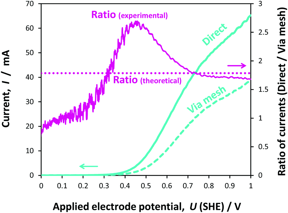 | ||
| Fig. 10 Oxygen evolution kinetics at a 0.1 × 0.1 m2 Ti|SnIV–Fe2O3 anode in 1 M NaOH solution recorded at a potential scan rate of 10 mV s−1 when illuminated directly and through the Ti|Pt cathode mesh; the ratio between the currents recorded for the two configurations, as well as the theoretical ratio based on the 56% open area of the mesh, are also shown. | ||
As expected, the photocurrent at the photo-anode with the configuration shown in Fig. 1(a) was greater than that for the configuration shown in Fig. 1(b), as the presence of the mesh between the light source and the hematite surface resulted in the attenuation of the photon flux. A 56% attenuation was estimated based on spectra measured with and without the mesh, resulting in the decrease in current by 1.79 times relative to the current measured in configuration (a). This was especially apparent at higher potentials. At lower potentials, the diversion from the theoretical value of 1.79 was attributed to lateral recombination, which would take place at the boundaries between the illuminated and shaded areas of the photo-anode, especially when Uapplied ≈ UFB. Hence, the ratio gradually increased from unity as the positive ‘overpotential’ was increased; at potentials negative of the flat band potential (+0.16(±0.022) V (SHE)), there was no difference between the currents as the photocurrent was negligible. The subsequent rise in the ratio above 1.79 in the region +0.3 ≤ Uapplied (SHE) ≤ +0.7 V was related to the scan rate, as demonstrated from the ratios computed from data obtained at scan rates of 10, 50 and 100 mV s−1 (Fig. 9S in the ESI‡); interestingly, the peak flattened with increasing scan rate.
It was concluded that the decrease in the current from case (a) to case (b) was almost exclusively caused by the decrease in the number of photons reaching the electrode surface. In principle, the extent of attenuation could be obviated by employing a mesh cathode with a larger open area, but mesh electrodes would suffer ohmic potential losses on scale-up, depending on current densities. The presence of a membrane or micro-porous separator, would cause additional attenuation.
The correlation between the geometry of the cathode and the decrease in current in configuration (b) relative to configuration (a), demonstrated that the effect was minimal of spatial inhomogeneities in the ionic current on the current measured on 0.1 × 0.1 m2 electrodes in configuration (a) in 1 M NaOH. This was not known a priori and demonstrated that the inhomogeneities in current distribution were minimal at operating geometric current densities below at least 6 A m−2 (computed from 60 mA using the geometric area of 0.01 m2).
Prediction of potential and current density distributions in the reactor
The effect of any inhomogeneities in the ionic current distribution in configuration (a) of Fig. 1 was studied further by comparing the experimental and simulated results with those for configuration (c). The numerical simulation was performed in COMSOL Multiphysics version 4.4, using the parameters listed in Table 2, together with previously defined boundary conditions and kinetic parameters specified in Table 1. We note that the light intensity, as well as the extent of light attenuation by the quartz in the larger reactor differed from that in the smaller reactor, due to the different light sources and their respective intensity spectra.| Parameter | Symbol | Value | Unit | Ref. |
|---|---|---|---|---|
| Un-attenuated light intensity incident on reactor (λ < 575 nm) | I | 4.36 × 10²⁰ | m−2 s−1 | This work |
| Spectrally resolved product of light intensity and absorption coefficient | ∑I0,λ·αλ | 3.08 × 1028 | m−3 s−1 | This work |
| Spectrally resolved product of light intensity and absorption coefficient (corrected for attenuation by quartz and electrolyte) | ∑(I0 − Ix)λ·αλ | 2.49 × 1028 | m−3 s−1 | This work |
| Exchange current density (H2O/O2 on α-Fe2O3) | j 0,anode | 5.56 × 10⁻³ | A m−2 | This work |
| Anodic Tafel coefficient (on α-Fe2O3) | β a | 0.295 | V dec−1 | This work |
| Exchange current density (H2O/H2 on Pt) | j 0,cathode | 3.1 | A m−2 | 31 |
| Electrolyte conductivity (1 M NaOH) |
σ
1MNaOH(25°C)
|
20.6 | A V−1 m−1 | This work |
| Titanium conductivity | σ Ti(25°C) | 1.8 × 10⁶ | A V−1 m−1 | 15 |
| Planar anode surface area | A planar | 10−2 | m2 | This work |
| Perforated surface area | A perforated | 8.6 × 10⁻³ | m2 | This work |
The modified Gärtner–Butler in eqn (16) was used to calculate the effect of applied photo-anode potential on photocurrent densities in terms of absorbed irradiance and electron–hole recombination rate for the two geometries. Dark current densities for the photo-anode were calculated from experimental voltammetric data obtained at 1 mV s−1 that fitted the Tafel equation well.
Fig. 11 shows the predicted local current density distribution for both a planar and a perforated photo-anode in 1 M NaOH. Higher current densities were predicted close to the edge of the planar electrode, but with a difference of only 0.08 A m−2 (2.9%) between maximum and minimum values. However, perforations helped to decrease this difference to 0.02 A m−2 (0.7%). It is evident that at this scale and with an electrolyte solution of 1 M NaOH, non-uniformity in current densities was predicted not to be an issue. Hence, the simulation results corroborated the conclusions drawn from comparison of experimental data collected for configurations (a) and (b) in Fig. 1. However, inhomogeneities in current density distribution may become an issue for larger electrodes or for electrolyte solutions with lower conductivities, resulting in less homogeneous distributions of potential in solution. For example, when that conductivity in the model was decreased notionally to 2 S m−1, while maintaining all other parameter values, a decrease of 0.71 A m−2 (25%) in the local current density was predicted along the surface of the planar 0.1 × 0.1 m2 photo-electrode, but only 0.17 A m−2 (6%) for the perforated photo-electrode. Hence, an a priori understanding of reactor performance may be achieved with this model which could greatly aid the design of reactors and explain their performance.
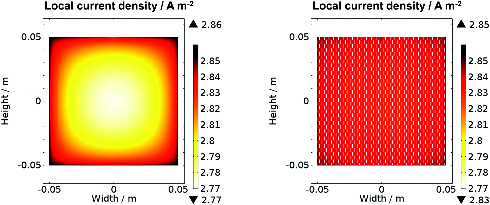 | ||
| Fig. 11 Secondary current density distribution at illuminated solid and perforated α-Fe2O3 surfaces in 1 M NaOH electrolyte as a function of spatial co-ordinates in the photo-electrochemical reactor at 0.7 V vs. SHE (1.5 V vs. RHE); modelled using COMSOL Multiphysics 4.4. | ||
Fig. 12 shows comparisons of experimental data with model predictions of the dependence on electrode potential of photocurrents at planar and perforated photo-electrodes, normalised with respect to the geometrical area of the electrode (0.01 m2) in 1 M NaOH. In the potential range 0.2–1.0 V (SHE), experimental current densities were not an exact match with their model counterparts. However, even such a match between the predictions, which were based on micro-kinetic parameters obtained at small electrodes, and experimental data collected at 0.1 × 0.1 m2 electrodes is rather extraordinary and falls well within the percentage error indicated in Fig. 9. There will always be differences, as even a scalable deposition processes like spray pyrolysis will yield different film thicknesses at small and large electrodes, for example due to temperature differences across substrate surfaces (caused by any substrate curvature that may be present), which affect solvent evaporation rates. Furthermore, larger light sources give rise to larger spatial intensity distributions, which will affect both the experimental performance and model predictions.
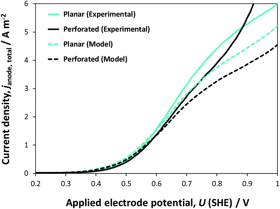 | ||
| Fig. 12 Comparison of effects of potential and electrode structure on experimental and predicted current densities for 0.1 × 0.1 m2 Ti|SnIV–Fe2O3 anode in 1 M NaOH solution; currents normalised by geometrical area of electrode. | ||
At potentials >0.9 V (SHE), higher current densities were obtained experimentally for the perforated photo-anode compared with those for the model prediction, probably because the areas inside the perforations were not insulated properly, as they were difficult to cover with lacquer to avoid increased dark currents.
The influence of perforations on current distributions became more pronounced as the electrolyte conductivity was decreased notionally by an order of magnitude, as evidenced from the comparison in Table 3 of current densities determined on planar and perforated electrodes in 1 M and 0.1 M NaOH solutions. Results are compared for measurements and simulations performed at an applied potential of +1.73 V (RHE) (corresponding to +0.91 V (SHE) in the 1 M NaOH electrolyte and +0.95 V (SHE) in the 0.1 M NaOH electrolyte).
| Parameter | 0.1 M NaOH | 1 M NaOH |
|---|---|---|
| Electrolyte conductivity, σ/A V−1 m−1 | 2.01 | 20.6 |
| pH | 13.3 | 13.9 |
| U FB/V (SHE) | 0.37 | 0.16 |
| Experimental – planar photo-anode: j/A m−2 | 2.81 | 4.59 |
| COMSOL model – planar photo-anode: j/A m−2 | 3.10 | 4.43 |
| Experimental – perforated photo-anode: j/A m−2 | 3.20 | 4.06 |
| COMSOL model – perforated photo-anode: j/A m−2 | 3.47 | 4.48 |
| Experimental – ratio of planar:perforated |
0.88 | 1.13 |
| COMSOL model – ratio of planar:perforated |
0.89 | 0.99 |
| Experimental – ratio of planar (0.1 M NaOH):planar (1 M NaOH) |
0.61 | |
| COMSOL model – ratio of planar (0.1 M NaOH):planar (1 M NaOH) |
0.70 | |
| Experimental ratio of perforated (0.1 M NaOH):perforated (1 M NaOH) |
0.79 | |
| COMSOL model ratio of perforated (0.1 M NaOH):perforated (1 M NaOH) |
0.77 | |
The comparison of ratios measured between planar and perforated electrodes showed that while inhomogeneity was not a significant issue in 1 M NaOH electrolyte, as evidenced from the ratio being ≈1, the impact of perforations certainly became pronounced as the electrolyte concentration and conductivity were decreased notionally by an order of magnitude, when the ratio becomes ≈0.89. This conclusion is supported by the simulations in COMSOL.
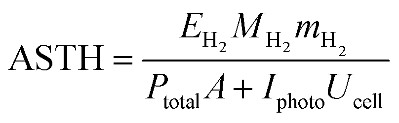
The above conclusion is supported further by experimental determination of the faradaic efficiencies of H2 evolution and also the assisted photon-to-hydrogen conversion efficiencies (ASTH) during 24 hour tests in a two-electrode arrangement. Faradaic efficiencies of H2 evolution,  , were computed from the ratio between the charge passed to generate the measured quantity of hydrogen to the total charge passed within a fixed time period (eqn (26)). The proposed formula for calculating solar to hydrogen efficiencies during assisted photo-electrolysis is shown in eqn (27).
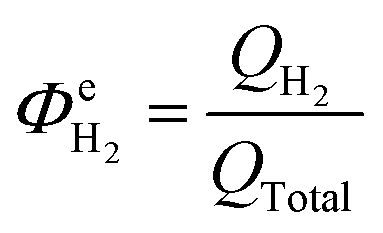 | (26) |
 | (27) |
In the first six to ten hours of reactor operation, several phenomena took place that significantly affected the  and ASTH values. Firstly, a proportion of the charge passed contributed towards the depletion of dissolved oxygen levels in the catholyte, as well as saturating the catholyte with H2. Secondly, the irradiation of the reactor resulted in the heating of the aqueous electrolyte. It was determined that 6 hours were required for the temperatures of both the anolyte and the catholyte to reach steady state values of 42.5 ± 2.5 °C. In order to ensure the reported values corresponded to steady state, we used only the data recorded during the second half of the 24 hour experiment.
Fig. 13 shows the faradaic efficiencies with which H2 was evolved at a Ti|Pt mesh cathode under steady state conditions during photo-assisted electrolysis at an applied cell potential difference of 1.6 V (corresponding to the photo-anode potential of +0.7 V (SHE)) with planar and perforated photo-anodes in 0.1 M and 1 M NaOH electrolytes. The average  values obtained during the 12 hour period are presented in Table 4. The charge and hydrogen gas volume measurements are presented in the ESI.‡
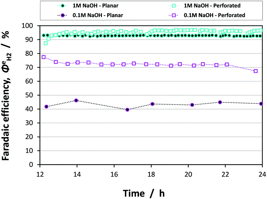 | ||
| Fig. 13 Faradaic efficiencies of H2 evolution at a Ti|Pt mesh cathode during photo-assisted electrolysis utilising planar and perforated 0.1 × 0.1 m2 hematite electrodes in 0.1 M and 1 M NaOH electrolytes. | ||
 ) and assisted solar-to-hydrogen conversion efficiencies obtained with planar and perforated 0.1 × 0.1 m2 electrodes in 0.1 M and 1 M NaOH electrolytes at an applied cell potential difference of 1.6 V
| Parameter | 0.1 M NaOH | 1 M NaOH |
|---|---|---|
 (planar)/% (planar)/% |
43.3(±2.5) | 93.2(±2.5) |
 (perforated)/% (perforated)/% |
73.0(±3.4) | 95.9(±3.0) |
| ASTH (planar)/% | 0.08(±0.01) | 0.83(±0.05) |
| ASTHgeometric (perforated)/% | 0.25(±0.01) | 0.79(±0.04) |
| ASTHactive (perforated)/% | 0.29(±0.02) | 0.91(±0.05) |
It is apparent that, within error, the faradaic H2 evolution efficiencies were the same for both the planar and perforated electrodes in 1 M NaOH solution. Hence, although the current density distribution is more homogeneous for the case of the perforated photo-anode as shown in Fig. 11, the effect of this on the H2 evolution efficiency was minimal in an electrolyte of high ionic strength/conductivity and at electrodes of 0.1 × 0.1 m2 scale. However, in the 0.1 M NaOH electrolyte, there was a stark difference between reactor performance with planar and perforated photo-absorbers. Firstly, the efficiencies for both the planar and perforated electrodes decreased significantly relative to the 1 M NaOH case; the decreased current density resulted in a greater proportion of charge being passed to reduce dissolved oxygen in the catholyte. Dissolved oxygen concentration would not be expected to decrease to zero with time due to the cross-over of dissolved oxygen from the saturated anolyte, so this problem will always affect steady state operation. Secondly, the difference between the planar and perforated case was due entirely to the conductivity of the electrolyte, resulting in non-uniform current density distribution in the planar case. The same conclusions may be drawn from the assisted solar-to-hydrogen conversion efficiencies presented in Table 4.
The findings qualitatively support the results of the experimental and numerical analysis of photo-current at the hematite photo-anodes under different conditions presented in Table 3. A direct numerical comparison is not appropriate here, as the faradaic efficiency of H2 evolution and H2–O2 cross-over have not been modelled and cannot be computed from the anodic photo-current density alone. Furthermore, photo-anode characterisation was carried out at 25 °C, whereas during steady state measurements, from which an ASTH was determined, the electrolyte temperature in the large reactor was 42.5 ± 2.5 °C. Further system modelling and investigation of water splitting kinetics as a function of temperature will be the subject of a subsequent manuscript.
The effect of electrode dimensions on the homogeneity of current distributions was further demonstrated via a 2D model of a 1.5 mm thick monolithic photo-bipole with length, ![[small script l]](https://www.rsc.org/images/entities/char_e146.gif) , in the range 10 mm to 1 m in 1 M NaOH. The model employed a configuration similar to that shown schematically in Fig. 1(d), while retaining geometrical similarity to the 3-D model in all directions for all sizes, including the volume of (1.0 M NaOH) electrolyte. Fig. 14 shows the spatial distribution of local current density as a function of electrode length at a fixed potential of +0.7 V vs. SHE (1.5 V vs. RHE), with all other parameter values the same as previously. As expected, the local current density along the electrode was predicted to decay with increasing length from an initial value of 2.7 A m−2, decreasing by 13% of that value at 0.1 m and 30% at 0.3 m. Consequently, while in 1 M NaOH the current distribution is not significant for 0.1 m electrodes, the decay in current density will become substantial on further scale-up.
, in the range 10 mm to 1 m in 1 M NaOH. The model employed a configuration similar to that shown schematically in Fig. 1(d), while retaining geometrical similarity to the 3-D model in all directions for all sizes, including the volume of (1.0 M NaOH) electrolyte. Fig. 14 shows the spatial distribution of local current density as a function of electrode length at a fixed potential of +0.7 V vs. SHE (1.5 V vs. RHE), with all other parameter values the same as previously. As expected, the local current density along the electrode was predicted to decay with increasing length from an initial value of 2.7 A m−2, decreasing by 13% of that value at 0.1 m and 30% at 0.3 m. Consequently, while in 1 M NaOH the current distribution is not significant for 0.1 m electrodes, the decay in current density will become substantial on further scale-up.
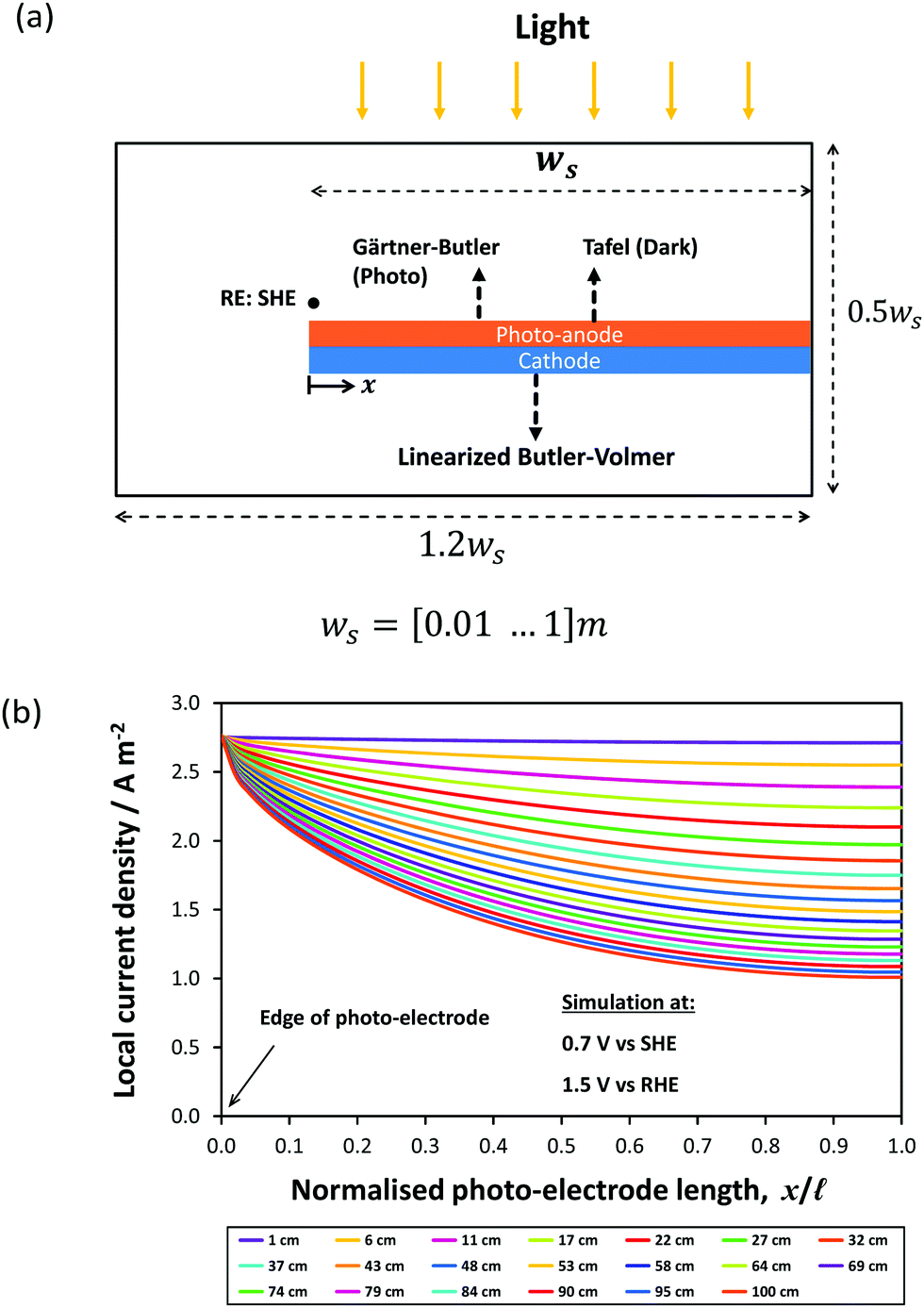 | ||
| Fig. 14 Predicted local current density distribution of Pt|Ti|SnIV–Fe2O3 photo-bipole under Xe arc lamp with power intensity of 312 W m−2 and 0.7 V vs. SHE (1.5 V vs. RHE). (a) Schematic view of the model and (b) predicted effect of photo-anode length on photocurrent density distributions. | ||
Finally, an ‘enhanced’ model photo-anode was evaluated as a component of a photo-bipole, but for an idealized case with a flat band potential UFB = 0 V vs. SHE, electron donor density of n0 = 1 × 1025 m−3, band gap of 1.7 eV and the absorbed photon flux (now, λ < 729 nm) was taken from AM 1.5 solar irradiance spectrum instead of the solar simulator, i.e., I0 = 1.21 × 10²¹ m−2 s−1. The electron–hole recombination kinetics (Fig. 6) in 1.0 M NaOH electrolyte solution were retained. Fig. 15 shows local current density distributions for different photo-bipole lengths up to 1.0 m, causing even sharper decays of local current density than shown in Fig. 11; from an initial value of circa 40 A m−2, local current densities were predicted to decrease by 78% of that value at 0.2 m from the edge. Hence, if more active photo-anodes are used instead of the α-Fe2O3 for which results are presented in this paper, inhomogeneities in current density distributions will be an even more important design issue when scaling-up reactors. Further complications may arise with lower electrolyte conductivities, when membrane/micro-porous separators are used to separate H2 and O2 evolved, and/or bubbles that reflect incoming photons are formed on electrode surfaces and that decrease conductivities of electrolyte solutions non-linearly with increasing gas fraction.
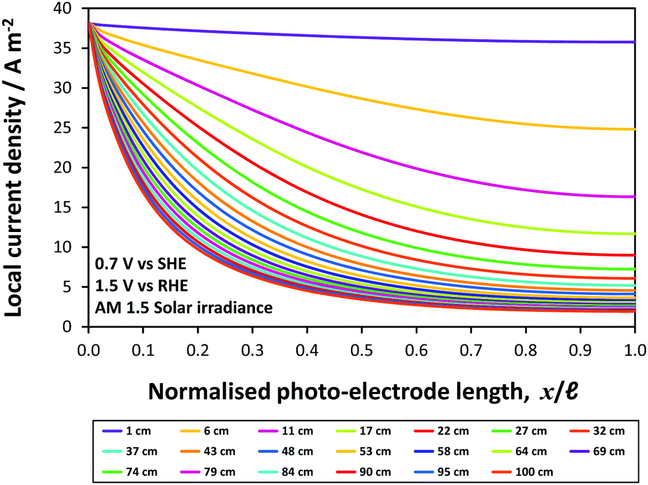 | ||
| Fig. 15 Predicted local current density distribution of ‘enhanced’ photo-bipole with Pt|Ti|photo-anode with Ebg = 1.7 eV under AM 1.5 solar irradiance at 0.7 V vs. SHE (1.5 V vs. RHE) in 1 M NaOH. | ||
In summary, it has been shown that current density distributions may limit device performance significantly, if the combined effects of electrode geometry/configuration and electrolyte conductivity are not considered prior to scale-up. Current density distributions will not have a pronounced effect on the faradaic efficiency and ASTH of H2 evolution at small electrodes (<0.1 × 0.1 m2 in size) and in concentrated (≥1 M) electrolytes. However, both the decrease in electrolyte conductivity and increase in electrode size in the direction of ionic current flow will result in current density distributions affecting device performance. Furthermore, as demonstrated in the ‘enhanced’ model, the importance of current density distributions also increases when better photo-absorbers and catalysts than hematite are employed.
The experimental and simulation results presented here were obtained in a type of reactor that is commonly referred to as a ‘wired’ device. In such a device, the (photo-)anode and (photo-)cathode are fabricated independently and integrated separately inside the reactor; hence, the electronic circuit is completed with the aid of a physical wire connecting the two electrodes. The alternative is a ‘wireless’ device in which the photo-absorbing and electro-catalyst elements are integrated in a monolithic assembly. Both device types can accommodate Z-scheme systems33–35 and photo-voltaic cells2,9,36,37 for solely solar-driven water splitting. However, current density distributions will affect both device designs and hence require careful analysis using the methods presented here and using an appropriate model of the photo-electrochemical kinetics. In integrated solar cells, careful consideration must be given to the spacing between the cells9 and/or electrode size;2 in wired devices, the relative electrode orientations and electrode geometry are of great importance, as demonstrated in this study. Ultimately, in the best performing device there will be a performance and cost-based optimisation of multiple factors, which include the choice of light absorber(s),10 catalysts, electrode geometry, electrolyte composition, electrolyte flow,13 reactor size and materials, product harvesting, method of photo-absorber illumination and intensity of illumination, which could be either non-concentrated or concentrated.38,39 Hence, accurate material characterisation as well as device modelling and optimisation, and the validation of such models in scaled systems, is essential to paving the way towards industrial deployment of photo-electrochemical devices.
Conclusions
The effect of electrode geometries and electrode configurations within a photo-electrochemical reactor have been predicted to affect the performance of photo-electrochemical reactors very significantly, especially on scale-up to electrodes with lengths >0.1 m, due to the spatial distributions of potential, photon flux and current densities, which were evaluated using finite element models. Decreasing electrolyte conductivities and increasing activities of photo-anodes caused greater inhomogeneities in the current density distributions. Including perforations in photo-electrodes was shown to offer a potential solution by decreasing ionic current path lengths and so decreasing macroscopic inhomogeneities in current density distributions, despite losses in effective absorber areas.A micro-kinetic model of oxygen evolution photocurrent based entirely on experimentally determined parameters: semiconductor film thickness, band gap, absorption coefficient, relative permittivity, charge carrier density, flat band potential and electron–hole recombination efficiencies, was validated against experimentally determined voltammograms, successfully describing data sets recorded at small and up-scaled (0.1 × 0.1 m2 in size) photo-electrodes.
Acknowledgements
The authors thank the UK Engineering and Physical Sciences Research Council for a studentships for CKO and JCA and a post-doctoral research associateship for AH, and COLCIENCIAS scholarship 567 for PhD studies abroad for FB.References
- T. Lopes, P. Dias, L. Andrade and A. Mendes, Sol. Energy Mater. Sol. Cells, 2014, 128, 399 CrossRef CAS.
- B. Turan, J.-P. Becker, F. Urbain, F. Finger, U. Rau and S. Haas, Nat. Commun., 2016, 7, 12681 CrossRef PubMed.
- J. J. H. Videira, K. W. J. Barnham, A. Hankin, J. P. Connolly, M. Leak, J. Johnson, G. H. Kelsall, K. Kennedy, J. S. Roberts, A. J. Cowan and A. J. Chatten, 2015, IEEE PVSC 42, 1.
- A. Berger and J. Newman, J. Electrochem. Soc., 2014, 161, E3328 CrossRef CAS.
- A. Berger, R. A. Segalman and J. Newman, Energy Environ. Sci., 2014, 7, 1468 CAS.
- M. E. Orazem and J. Newman, J. Electrochem. Soc., 1984, 131, 2582 CrossRef CAS.
- M. E. Orazem and J. Newman, J. Electrochem. Soc., 1984, 131, 2857 CrossRef CAS.
- S. Haussener, C. Xiang, J. M. Spurgeon, S. Ardo, N. S. Lewis and A. Z. Weber, Energy Environ. Sci., 2012, 5, 9922 CAS.
- S. Haussener, S. Hu, C. Xiang, A. Z. Weber and N. S. Lewis, Energy Environ. Sci., 2013, 6, 3605 CAS.
- S. Hu, C. Xiang, S. Haussener, A. D. Berger and N. S. Lewis, Energy Environ. Sci., 2013, 6, 2984 CAS.
- A. A. Akl, Appl. Surf. Sci., 2004, 233, 307 CrossRef CAS.
- ASTM, ASTM G173-03 Standard Tables for Reference Solar Spectral Irradiances: Direct Normal and Hemispherical on 371 Tilted Surface, 2012.
- C. Carver, Z. Ulissi, C.-K. Ong, S. Dennison, K. Hellgardt and G. H. Kelsall, ECS Trans., 2010, 28, 103 CAS.
- C. K. Ong, S. Dennison, S. Fearn, K. Hellgardt and G. H. Kelsall, Electrochim. Acta, 2014, 125, 266 CrossRef CAS.
- R. W. Powell and R. P. Tye, J. Less-Common Met., 1961, 3, 226 CrossRef CAS.
- S. Y. Reece, J. A. Hamel, K. Sung, T. D. Jarvi, A. J. Esswein, J. J. H. Pijpers and D. G. Nocera, Science, 2011, 334, 645 CrossRef CAS PubMed.
- P. Carmichael, D. Hazafy, D. S. Bhachu, A. Mills, J. A. Darr and I. P. Parkin, Phys. Chem. Chem. Phys., 2013, 15, 16788 RSC.
- B. Neumann, P. Bogdanoff and H. Tributsch, J. Phys. Chem. C, 2009, 113, 20980 CAS.
- K. G. Upul Wijayantha, S. Saremi-Yarahmadi and L. M. Peter, Phys. Chem. Chem. Phys., 2011, 13, 5264 RSC.
- G. H. Kelsall and R. A. Williams, J. Electrochem. Soc., 1991, 138, 931 CrossRef CAS.
- W. W. Gärtner, Phys. Rev., 1959, 116, 84 CrossRef.
- M. A. Butler, J. Appl. Phys., 1977, 48, 1914 CrossRef CAS.
- L. M. Peter, J. Solid State Electrochem., 2013, 17, 315 CrossRef CAS.
- B. Klahr, S. Gimenez, F. Fabregat-Santiago, T. Hamann and J. Bisquert, J. Am. Chem. Soc., 2012, 134, 4294 CrossRef CAS PubMed.
- N. Sato, Electrochemistry at Metal and Semiconductor Electrodes, Elsevier, Amsterdam, 1998 Search PubMed.
- A. Hankin, J. C. Alexander and G. H. Kelsall, Phys. Chem. Chem. Phys., 2014, 16, 16176 RSC.
- S. Onari, T. Arai and K. Kudo, Phys. Rev. B: Solid State, 1977, 16, 1717 CrossRef CAS.
- J. H. Kennedy and K. W. Frese, Jr., J. Electrochem. Soc., 1978, 125, 723 CrossRef CAS.
- R. K. Quinn, R. D. Nasby and R. J. Baughman, Mater. Res. Bull., 1976, 11, 1011 CrossRef CAS.
- IUPAC. Compendium of Chemical Terminology, 2nd edn, (the “Gold Book”). Compiled by A. D. McNaught and A. Wilkinson, Blackwell Scientific Publications, Oxford, UK, 1997.
- P. Ekdunge, K. Jüttner, G. Kreysa, T. Kessler, H. Ebert and W. J. Lorenz, J. Electrochem. Soc., 1991, 138, 2660 CrossRef CAS.
- Z. Chen, T. F. Jaramillo, T. G. Deutsch, A. Kleiman-Shwarsctein, A. J. Forman, N. Gaillard, R. Garland, K. Takanabe, C. Heske, M. Sunkara, E. W. McFarland, K. Domen, E. L. Miller, J. A. Turner and H. N. Dinh, J. Mater. Res., 2010, 25, 3 CrossRef CAS.
- H. S. Park, H. C. Lee, K. C. Leonard, G. Liu and A. J. Bard, ChemPhysChem, 2013, 14, 2277 CrossRef CAS PubMed.
- M. Grätzel, Nature, 2001, 414, 338 CrossRef PubMed.
- F. E. Osterloh and B. A. Parkinson, MRS Bull., 2011, 36, 17 CrossRef CAS.
- T. J. Jacobsson, V. Fjällström, M. Edoff and T. Edvinsson, Energy Environ. Sci., 2013, 6, 3676 CAS.
- T. J. Jacobsson, V. Fjällström, M. Sahlberg, M. Edoff and T. Edvinsson, Energy Environ. Sci., 2014, 7, 2056 CAS.
- S. Tembhurne and S. Haussener, J. Electrochem. Soc., 2016, 163, H988 CrossRef CAS.
- S. Tembhurne and S. Haussener, J. Electrochem. Soc., 2016, 163, H999 CrossRef CAS.
Footnotes |
| † The underlying research data for this paper is available in accordance with EPSRC open data policy from http://zenodo.org/record/200501#.WFA237KLTct |
| ‡ Electronic supplementary information (ESI) available. See DOI: 10.1039/c6ee03036j |
| § Current address: PIPDEV Ltd., PO Box 36522, London W4 2XF, UK. |
| ¶ Current address: Arup, 13 Fitzroy St, London W1T 4BQ, UK. |
| || Current address: Syngenta, 4002 Basel, Switzerland. |
| This journal is © The Royal Society of Chemistry 2017 |