Correlating geminal 2JSi–O–Si couplings to structure in framework silicates†
Received
21st September 2017
, Accepted 21st November 2017
First published on 29th November 2017
Abstract
The dependence of a 29Si geminal J coupling across the inter-tetrahedral linkage on local structure was examined using first-principles DFT calculations. The two main influences on 2JSi–O–Si were found to be a primary dependence on the linkage Si–O–Si angle and a secondary dependence on mean Si–O–Si linkage of the two coupled 29Si nuclei. An analytical expression describing these dependences was proposed and used to develop an approach for relating the correlated pair of 2JSi–O–Si coupling and mean 29Si isotropic chemical shift to the linkage Si–O–Si angle and the mean Si–O–Si angle of the two coupled 29Si nuclei. An example of this analysis is given using 29Si NMR results from the siliceous zeolite Sigma-2.
1 Introduction
The isotropic chemical shift of 29Si NMR has long been a valuable probe of structure in silicate materials.1–4 In changing coordination from SiO4 to SiO5 to SiO6 the chemical shift range of 29Si in silicates varies from approximately −100 to −150 to −200 ppm, respectively.5 In the case of tetrahedral coordination, the chemical shift varies over a range of −120 to −70 ppm as the second coordinate sphere changes from fully connected Q4 to fully disconnected Q0, respectively.6 For Q4 sites it is well established that variations in the range of −105 ppm to −120 ppm in the isotropic chemical shift of 29Si are correlated to the mean of the Q4's four inter-tetrahedral angles.7–9
The anisotropy of the 29Si chemical shift is also strongly correlated to changes in the first-coordination sphere. As first noted by Grimmer and coworkers,10,11 as the Si–O bond length decreases there is an increase in the s-character of the bonding orbital at Si and corresponding increase in shielding along the direction of the shorter bond. This strong dependence of the 29Si chemical shift anisotropy has been exploited not only for distinguishing and quantifying Qn sites,12–16 but recently has been found to be an effective probe of the modifier cation coordination to the non-bridging oxygen of Q3 sites17 and useful in the NMR refinement of crystal structures.18
In contrast to the 29Si chemical shift, accurate measurements of geminal 2JSi–O–Si couplings across the inter-tetrahedral linkage in silicates have yielded no clear relationships between coupling constant and local structure. While 2JSi–O–Si couplings in solution have been measured,19–23 motional averaging makes it difficult to use these measurements to establish empirical relationships. The number of 2JSi–O–Si measurements in solids have been limited, particularly at 29Si natural abundance levels, 4.67%, and thus far few efforts24–26 have been made in trying to establish quantitative relationships between 2JSi–O–Si and structure. Compounding this issue is that commercial computational chemistry packages have only recently reached the level where accurate J-couplings can be calculated through using expensive density function theory (DFT) methods.27 Nevertheless, geometric dependences have been reproduced using modest DFT calculations. The most recent attempts in determining such relationships, using ab initio DFT methods, were in 2009 by Cadars et al.26 and Florian et al.25 Although both groups acknowledged a dependence of 2JSi–O–Si coupling on Si–O–Si bond angle, Florian et al. suggested a one-to-one mapping, whereas Cadars et al. found that the dependence of the 2JSi–O–Si coupling is not limited to the Si–O–Si bond angle but is also influenced significantly by the local geometry around the Si–O–Si linkage. Cadars et al. concluded that such dependencies led to a relatively “large scatter” of 2JSi–O–Si coupling, with respect to Si–O–Si bond angle, and did not attempt to deduce any empirical relationship between the 2JSi–O–Si coupling and the local structure. To get a sense of that scatter, we plot the 2JSi–O–Si couplings—calculated here—as a function of Si–O–Si bond angle in Fig. S5 of the ESI.†
Here we re-examine the variation in 2JSi–O–Si using Q4–Q4 clusters that are centered on the Si–O–Si linkage extending out to four coordination spheres away from the bridging oxygen between the two coupled silicon. With greater computational resources than were available to Cadars et al. 8 years ago, we were able to increase the level of theory and obtain excellent agreement with known experimental 2JSi–O–Si couplings. Through systematic structural variations of the cluster, we investigated the influence of (1) the Si–O–Si linkage angle, (2) the Si–O bond distance, (3) the inter-tetrahedral dihedral angle, and (4) the outer Si–O–Si linkage angles of the two coupled 29Si nuclei. Most significantly we show here that after the central Si–O–Si linkage angle it is the outer Si–O–Si linkage angles of the Q4–Q4 couple that play the next most significant role in determining 2JSi–O–Si. A smaller dependence on the dihedral angle is observed while a negligible dependence on Si–O distance over relevant length scales is observed. In this study we assume the SiO4 tetrahedron does not deviate from local tetrahedral symmetry and take the intra-tetrahedral O–Si–O angle as constant. While this is a reasonable approximation in a fully connected Q4 network, it is likely that this assumption will break down as the silicate network becomes depolymerized. Further work will be required to understand the dependence of J coupling on local structure in networks having significant distortions around SiO4 tetrahedra.
As the isotropic chemical shift has a well known dependence on the mean Si–O–Si angle, we also show here that a correlation plot of mean 29Si isotropic chemical shift versus2JSi–O–Si coupling can be mapped into a two dimensional structural correlation of linkage Si–O–Si angle to mean Si–O–Si angle of the two coupled 29Si nuclei.
2 Method
All ab initio calculations were carried out using Gaussian 0928 at the Ohio supercomputing center,29 running HP SL390 G7 two-socket servers with Intel Xeon x5650 (Westmere-EP, 6 core, 2.67 GHz) processors and 48 GB memory. The natural atomic orbital and natural bond orbital analysis was performed using Gaussian NBO version 3.1.30 The 2JSi–O–Si couplings were calculated using DFT with B3LYP functional on a small O centered SiH3 terminated cluster, (H3SiO)3–Si–O–Si–(OSiH3)3, shown in Fig. 1. A perfect tetrahedron angle ∠O–Si–O = 109.5° was imposed about Si atoms in all calculations.
 |
| | Fig. 1 (H3SiO)3–Si–O–Si–(OSiH3)3 symmetric cluster used in calculating the 2JSi–O–Si coupling across Si(i)–O–Si(j). | |
A locally dense basis set was implemented on this cluster, as suggested by Cadars et al.,26 for accurate 2JSi–O–Si coupling calculations. This follows an implementation of cc-PV5Z basis set on the two central Si (labeled Si(i) and Si(j) in Fig. 1), 6-31++G basis set on all H, and 6-31++G* basis set on all O and remaining Si. Single point NMR calculations were run with tight self consistent field (SCF) convergence criteria. The integration grid size was increased to a pruned (99, 590), ‘ultrafine’ grid, although no differences in 2JSi–O–Si couplings were observed from the pruned (75, 302) ‘fine’ integration grid. All further calculations were, therefore, subjected to a ‘fine’ integration grid. With this setup each calculation took approximately four and a half hours split over 12 cpu cores.
Systematic structural variations of the cluster were performed to investigate the 2JSi–O–Si coupling dependence on and correlations between the central Si–O–Si bond angle, Ω0, and (a) Si–O bond distances, dSi–O, (b) O–Si–Si–O inter-tetrahedral dihedral bond angle, ϕ (index O1–Si(i)–Si(j)–O4 in Fig. 1) and (c) outer Si–O–Si bond angles (Ω1 to Ω6). With the geometry constrained out to the third coordination sphere of the central linkage oxygen, a geometry optimization of the outermost Si–H bond distances and the remaining dihedral angles was performed once using restricted Hartree–Fock, RHF/6-311G(d) basis set. We found, as did Cadars et al.,26 that variations in these fourth coordination sphere geometries had negligible effect on the predicted J-coupling. We confirmed this finding with several 2JSi–O–Si coupling calculation starting with RHF/6-311G(d) optimized initial geometries and the results are tabulated in Table S3 of the ESI.† A complete list of all geometrical constraints imposed in this study is tabulated in Tables S1–S5 of the ESI.†
Si–O bond distance, dSi–O
The 2JSi–O–Si coupling dependence on and correlation between Ω0 and dSi–O was explored by performing a series of 2JSi–O–Si coupling calculations on the optimized structure by varying Ω0 from 120° to 180° on a uniform grid for three Si–O bond distances, dSi–O = 1.58 Å, 1.60 Å and 1.62 Å, respectively, Fig. 2C.
 |
| | Fig. 2 Dependence and correlation of 2JSi–O–Si couplings between Si(i)–O–Si(j) bond angle, Ω0 and (A)  , (B) O–Si–Si–O inter tetrahedral dihedral angle, ϕ and (C) Si–O bond distance, dSi–O. For calculations in (A) dSi–O = 1.60 Å and Ωk≠0 = Ωout varied from 120° to 180°. In (B) dSi–O = 1.60 Å, Ωout = 146° and ϕ varied from −60° to +60°. In (C) Ωout = 146° and d varied from 1.58 Å to 1.62 Å. , (B) O–Si–Si–O inter tetrahedral dihedral angle, ϕ and (C) Si–O bond distance, dSi–O. For calculations in (A) dSi–O = 1.60 Å and Ωk≠0 = Ωout varied from 120° to 180°. In (B) dSi–O = 1.60 Å, Ωout = 146° and ϕ varied from −60° to +60°. In (C) Ωout = 146° and d varied from 1.58 Å to 1.62 Å. | |
O–Si–Si–O dihedral angle, ϕ
A similar series of calculations were performed on the optimized geometry to investigate the 2JSi–O–Si coupling dependence on and correlation between Ω0 and ϕ. This was accomplished by independently varying ϕ and Ω0 from −60° to +60° and 120° to 180°, respectively, Fig. 2B. All Si–O bond distances were set to 1.6 Å.
Outer Si–O–Si bond angle, Ωk≠0
A complete systematic exploration of the 2JSi–O–Si dependence on the six outer Si–O–Si bond angles would have exceeded our computational capabilities. In light of the well established8 linear dependence of the isotropic 29Si chemical shift on the mean Si–O–Si bond angle for a Q4 tetrahedra we attempted to reduce the dimensionality of the problem by using the mean Si–O–Si bond angle for each Q4 tetrahedra, (Si(i) and Si(j)) involved in the 2JSi–O–Si coupling, that is,| |  | (1) |
to calculate a double mean| |  | (2) |
Through systematic variation of Ω0 (the central linkage angle) and  we show (vide infra) that a combined measurement of isotropic 29Si chemical shift and 2JSi–O–Si can be exploited to determine the local structure around the Q4–Q4 linkage.
Despite this effort to reduce the dimensionality of this problem from seven to two, there still exist infinite combinations of Ωk≠0 that lead to the same  in eqn (2), with the exception of the singular—and highly unlikely—occurrence of
  . To ensure a systematic variation of the local structure, we choose to constrain all Ωk≠0 = Ωout. A series of 2JSi–O–Si calculations were performed by independently vary Ωout and Ω0 from 120° to 180° on a uniform grid. The calculated 2JSi–O–Si as a function of
  and Ω0 is presented in Fig. 2A. All Si–O bond distances were set to 1.6 Å. Of course, the constraint Ωk≠0 = Ωout, implemented only to ensure a systematic local structural variation, is unrealistic even for most crystalline silicates and highly siliceous zeolites, as well as in silica glass and other silica rich disordered materials. To break free from this constraint numerous 2JSi–O–Si coupling calculations were performed at arbitrary outer Si–O–Si bond angles Ωk≠0 and ϕ, with values listed in Tables S3 and S4 of the ESI.† These calculations are used to further verify agreement with our proposed 2JSi–O–Si coupling model.
All additional numerical analysis codes were written in python using NumPy libraries.31 The least square analysis was performed using python's LMFIT32 module. The graphics were produced using python's matplotlib library.33
3 Theory
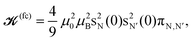
The J coupling contribution to the nuclear spin Hamiltonian can be written34| | ĤJ = ![[small mu, Greek, circumflex]](https://www.rsc.org/images/entities/i_char_e0b3.gif) N· N·![[scr K, script letter K]](https://www.rsc.org/images/entities/b_char_e148.gif) ·N′ = ℏ2γNγN′ÎN··ÎN′. ·N′ = ℏ2γNγN′ÎN··ÎN′. | (3) |
The convention is to combine the gyromagnetic ratio constants and the reduced tensor such thatwith| |  | (5) |
This gives a J tensor with dimensions of inverse time.
As we explored the calculated variations in 2JSi–O–Si with changing cluster structure, we searched for the possible empirical relationships that might characterize the observed correlation of 2JSi–O–Si to structure. In our calculations we found that the majority of the J-coupling arises from the Fermi contact (FC) contribution, and the remaining contributions from spin–dipolar (SD), paramagnetic spin–orbit (PSO), and diamagnetic spin–orbit (DSO), as illustrated in Fig. S2 of the ESI,† account for less than 10% of the net J-coupling. With this in mind, we looked for guidance in the older literature of J coupling theory and focused on the simple and highly approximate MO theory approach outlined by Pople and Santry,35–40 which considers only the isotropic Fermi contact contribution and yields the expression
| |  | (6) |
where
μ0 is the magnetic constant,
μB is the Bohr magneton, s
N(0) and s
N′(0) are the values of the valence s-orbitals of atoms N and N′ at the nuclei, and π
N,N′ is the mutual atom–atom polarizability of Coulson and Longuet-Higgins,
41 given by
| |  | (7) |
Here the summation is over occupied (
i) and unoccupied (
j) molecular orbitals, |
ψi〉, with energy
εi and given by
| |  | (8) |
which are expressed in terms of the valence hybrid type orbitals (HTOs), |
ϕμ〉, which are given by
| | | |ϕμ〉 = aμ|s〉 + (1 − a2μ)1/2|p〉, | (9) |
where |s〉 and |p〉 are the atomic-type orbitals and
a2μ is the s-character of the HTO. In the summation of
eqn (7) the
μ and
ν index the HTOs on N and N′, respectively.
An exhaustive search of the literature reveals few MO theory studies considering the geminal 2JAB coupling between tetrahedrally coordinated atoms. The most relevant and detailed discussion we could find on this topic is a chapter in 1988 by Klessinger and Barfield,42 examining the dependence of geminal 13C–13C coupling constants. In this case they derive the mutual atom–atom polarizability as
| |  | (10) |
where
a21 and
a23 are the s-character of the HTOs at carbon C
1 and C
3 along C–C bond directed towards C
2, in a C
1–C
2–C
3 linkage. The integral
βμ,ν is the matrix element of the Hamiltonian operator in the HTO basis set |
ϕμ〉,
The definition of these integrals are given in Klessinger and Barfield.
42 If all integrals in
eqn (10) except

are ignored, the mutual atom–atom polarizability term can be approximated
42 to
where
a22 is the s-character of the valence HTO at C
2. The
2JC1,C3 can then be approximated to
While
eqn (13) predicts a simple linear correlation of
2JC1,C3 to the s-character product, we expect this highly approximated correlation to deviate from linearity due to the neglect of the vicinal integrals.
42 Nevertheless, this approximate model provides a useful starting point for developing an empirical expression for geminal
J coupling across two coupled
29Si. On the basis of
eqn (13), we propose that
2JSi–O–Si is approximately given by
| |  | (14) |
where

and

are the products of the s-character of the valence HTOs associated with the Si
(i)–O and Si
(j)–O bonds across Si
(i)–O–Si
(j) linkage, respectively, as illustrated in
Fig. 3.
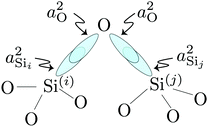 |
| | Fig. 3 Simple illustration of valence HTOs associated with the Si(i)–O and Si(j)–O bonds across Si(i)–O–Si(j) linkage. | |
4 Results and discussion
4.1 Dependence on local structure
In this subsection, we discuss and examine the contributions to the net 2JSi–O–Si coupling arising from the variations in the local structure on the basis of the underlying s-characters a2O,  , and
, and  at the bridging oxygen and adjacent silicons respectively. These values were determined from the quantum chemistry DFT cluster calculation using Gaussian NBO version 3.1. For clarity, we only present a subset of results from Fig. 2 per structural parameters considered.
Shown in Fig. 4A is the expected dependence of 2JSi–O–Si coupling on Ω0 ∈ [120°,180°], for a subset of results from Fig. 2A where the outer Si–O–Si angles are held constant at Ωk≠0 = 180° and the distances held constant at dSi–O = 1.6 Å. This dependence of 2JSi–O–Si coupling on the Si–O–Si linkage angle, Ω0, has been previously discussed by both Cadars et al.26 and Florian et al.25 In Fig. 4B we see the more intriguing result that the 2JSi–O–Si coupling has a markedly linear correlation to the product  , as predicted by eqn (14). As noted earlier, the slight deviation from linearity observed is not unexpected and is likely attributed to the neglected terms in the mutual atom–atom polarizability term. In Fig. 4C and D we see that the variation in 2JSi–O–Si primarily arises from variation in a4O,—the s-character product of the two valence HTOs at the bridging oxygen—while there is a minor yet non-negligible variation coming from
  —the s-character product of the two silicon valence HTOs in the Si–O–Si linkage. The change in a4O is the result of the change in the hybridization of the valence orbitals at the bridging oxygen from sp2 (33.33% s-character) at Ω0 = 120° to sp (50% s-character) at Ω0 = 180°. A popular approximation for the s-character at the bridging oxygen9,42 is given by
| |  | (15) |
Here we use the symbol
fO(
Ω) to distinguish the approximated s-character at the bridging oxygen from the symbol
a2O for the s-character calculated using quantum chemistry DFT calculations.
 |
| | Fig. 4 Dependence of 2JSi–O–Si coupling on (A) Si–O–Si bond angle Ω0, (B)  , (C) a4O, and (D) , (C) a4O, and (D)  for the constraints Ωk≠0 = 180° and d = 1.6 Å. for the constraints Ωk≠0 = 180° and d = 1.6 Å. | |
With the s-character of each sp3 valence HTO on a tetrahedral silicon expected to be 25%, the calculated value of  is also as expected at ∼(25%)2 = 6.25%. The slight increase in
  from 6.1% to 6.7% in Fig. 4D with decreasing Ω0 may seem surprising from a simple hybrid orbital picture—as all intra-tetrahedral angles and Si–O distances are held constant at ∠O−Si−O = 109.5° and dSi–O = 1.6 Å, respectively, in these calculations. In fact, for this subset of results, even the outer Si–O–Si angles are held fixed at 180°, so it is only the variation of the linkage angle Ω0 that is responsible for this slight change in
  . We will examine the origin of this variation shortly when the influence of the outer Si–O–Si angles on 2JSi–O–Si are considered.
In Fig. 5A is the variation of 2JSi–O–Si with the two central linkage Si–O bond distances, dSi–O ∈ [1.58 Å, 1.62 Å], for a subset of results from Fig. 2C where the central linkage angle was fixed at Ω0 = 180° and the outer Si–O–Si angles and outer distances are held constant at Ωk≠0 = 146° and dSi–O = 1.6 Å, respectively. The 2JSi–O–Si coupling remains relatively constant around 21.5 Hz over this range of central linkage Si–O bond distances, with a slight decrease from ∼22 to ∼21 Hz with increasing bond length. This relative independence of 2JSi–O–Si on the central linkage Si–O bond distances is consistent with previous observations by Florian et al.25 In Fig. 5B we find again that the 2JSi–O–Si coupling has a linear correlation to the product  , and in Fig. 5C we see no observable dependence of 2JSi–O–Si coupling on the s-character product a4O at the bridging oxygen. This is because, for this subset of calculations, the hybridization at the bridging oxygen was locked to sp through the constraint Ω0 = 180°. Since the s-character at the bridging oxygen predominantly depends on the Si–O–Si bond angle, as noted in eqn (15), the change in Si–O bond distance, dSi–O, shows no observable change in its s-character. In Fig. 5D we find that the minor variation in 2JSi–O–Si coupling is dominated by the change in
  . While a decrease in the a2Si with increasing Si–O bond distance has been previously reported by Grimmer and coworkers10,11 it was in the context of correlated changes in the intra-tetrahedral angle ∠O–Si–O. With the intra-tetrahedral angles in this calculation fixed at ∠O–Si–O = 109.5°, it seems that changes in Si–O length alone lead to minor variations in a2Si—although these result in relatively insignificant variations in 2JSi–O–Si.
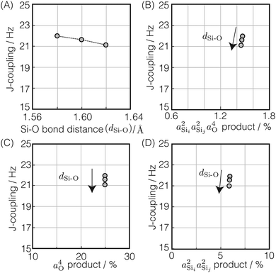 |
| | Fig. 5 Dependence of 2JSi–O–Si coupling on (A) Si–O bond distance, dSi–O, (B)  , (C) a4O, and (D) , (C) a4O, and (D)  for the constraints Ω0 = 180° and Ωk≠0 = 146°. for the constraints Ω0 = 180° and Ωk≠0 = 146°. | |
In Fig. 6A is the variation of 2JSi–O–Si with the inter-tetrahedral dihedral angle ϕ ∈ [−60°,60°] for a subset of results from Fig. 2B where the central linkage angle was fixed at Ω0 = 180°, and the outer Si–O–Si angles and outer distances are held constant at Ωk≠0 = 146° and dSi–O = 1.6 Å, respectively. A periodic modulation of the form cos![[thin space (1/6-em)]](https://www.rsc.org/images/entities/char_2009.gif) 3ϕ for 2JSi–O–Si over a range of 1.6 Hz is observed due to the local three fold symmetry of the (H3SiO)3–Si–O–Si–(OSiH3)3 cluster when rotating about ϕ. There is no observable variation in the hybrid orbital s-character products in Fig. 6B–D as expected, since this variation is associated with the vicinal integral terms of the mutual atom–atom polarizability expansion which are completely neglected in eqn (14).
3ϕ for 2JSi–O–Si over a range of 1.6 Hz is observed due to the local three fold symmetry of the (H3SiO)3–Si–O–Si–(OSiH3)3 cluster when rotating about ϕ. There is no observable variation in the hybrid orbital s-character products in Fig. 6B–D as expected, since this variation is associated with the vicinal integral terms of the mutual atom–atom polarizability expansion which are completely neglected in eqn (14).
 |
| | Fig. 6 Dependence of 2JSi–O–Si coupling on (A) O–Si–Si–O inter tetrahedral dihedral angle, ϕ, (B)  , (C) a4O, and (D) , (C) a4O, and (D)  for the constraints Ωk≠0 = 146°, Ω0 = 180° and d = 1.6 Å. for the constraints Ωk≠0 = 146°, Ω0 = 180° and d = 1.6 Å. | |
In Fig. 7A is the variation of 2JSi–O–Si with  , as calculated by eqn (2), for a subset of results from Fig. 2A subjected to the constraint Ω0 = 180°, Ωk≠0 = Ωout and d = 1.6 Å where Ωout varied from 120° to 180°. The variation in Fig. 7A is about 25% of that shown in Fig. 4A and is found to be the second most dominant dependence of 2JSi–O–Si coupling. As Ω0 is fixed, it is the change in the outer Si–O–Si bond angles, Ωout, that leads to this variation in 2JSi–O–Si. In Fig. 7B we again find the markedly linear correlation of 2JSi–O–Si coupling with
  as predicted by eqn (14). As might be expected, no observable dependence of 2JSi–O–Si coupling on a4O is observed in Fig. 7C since the hybridization at the bridging oxygen was fixed to sp with the constraint Ω0 = 180°.
 |
| | Fig. 7 Dependence of 2JSi–O–Si coupling on (A) the average Si–O–Si bond angles,  , (B) , (B)  , (C) a4O, and (D) , (C) a4O, and (D)  for the constraints Ω0 = 180° and d = 1.6 Å. for the constraints Ω0 = 180° and d = 1.6 Å. | |
Clearly, the origin of the 2JSi–O–Si dependence on the outer angles, Ωout comes from the variation in  as seen in Fig. 7D. Why would the
  or
or  increase as the outer angles, Ωout, increase? This is the same question alluded to earlier with respect to Fig. 4D. The logic is as follows. We expect the sum of the s-characters for the four HTO around each silicon to be constant. So, as the s-character of one HTO deviates from 25%, the s-characters of the other HTO compensate to maintain the constant sum. Hence, we expect the s-character of the HTO that is part of the central linkage to increase as the average s-character of the other three HTOs decreases. Close examination of the variation in
  as the function of the Si–O–Si tetrahedral angle, Ω0, and average Si–O–Si bond angle, 〈Ω〉i, also shown in Fig. S3 of the ESI,† reveals an approximate proportionality given by
| |  | (16) |
In regard to
Fig. 4D, since the outer Si–O–Si bond angles are held constant,
Ωk≠0 = 180°, the individual s-characters at Si
(i) and Si
(j) and, therefore, the product,

, decreases as
Ω0 increases.
The highly approximate J-coupling model in eqn (14) predicts a linear correlation of 2JSi–O–Si coupling with respect to the s-character product,  . From the ab initio calculations, shown in Fig. 8, however, we find that the 2JSi–O–Si coupling is better described by a quadratic in the s-character product,
  , with R2 = 0.99164. As mentioned earlier, this slight curvature is not unexpected, since the model in eqn (14) neglects all the vicinal integrals from the mutual atom–atom polarizability term. Further discussion on the effect of vicinal integrals can be found in the chapter by Klessinger and Barfield.42
 |
| | Fig. 8
2
J
Si–O–Si coupling as a function of  at Si(i), Si(j) and O across Si(i)–O–Si(j) linkage. The points in gray and black corresponds to the systematic (Ωk≠0 = Ωout) and arbitrary structural variations, respectively. at Si(i), Si(j) and O across Si(i)–O–Si(j) linkage. The points in gray and black corresponds to the systematic (Ωk≠0 = Ωout) and arbitrary structural variations, respectively. | |
Fig. 8 shows the 2JSi–O–Si couplings in two different colors, gray and black. The gray dots correspond to couplings evaluated by systematic variation of the local structure, also shown in Fig. 2, and are provided in the Tables S1 and S2 of the ESI.† The black dots correspond to couplings evaluated at arbitrary Ωk and ϕ and are listed in Tables S3 and S4 of the ESI.† Most notably a consistent trend in 2JSi–O–Si is observed with respect to the s-character product,  , for both systematic and arbitrary structural variation.
On the basis of the results and discussion presented here we can now construct an expression relating 2JSi–O–Si to local structure. The most straightforward approach would be a substitution of eqn (15) and (16) into eqn (14). We found, however, that such an approach leads to an excessive number of coefficients for calibrating the relationship. Instead we found that the same relationship can be expressed with fewer coefficients using
| |  | (17) |
For this expression the coefficients
m1 = 0.778 ± 0.004 Hz per °,
m2 = 0.0058 ± 0.0005 Hz per ° and
J0 = −8.3 ± 0.1 Hz were determined by least square minimization of the objective function
| |  | (18) |
Note there is a strong cross correlation coefficient
ρm1,J0 = −0.918 between
m1 and
J0 in this determination. A comparison of
ab initio2JSi–O–Si couplings with respect to the
2JSi–O–Si coupling model in
eqn (17) is presented in
Fig. 9A. Again, the points in gray and black correspond to systematic and arbitrary variation of the local structure, respectively. Excellent agreement between the
2JSi–O–Si coupling model and
2JSi–O–Si coupling from
ab initio calculation is observed with
R2 = 0.99518. Note that in this approach the slight dependence on Si–O bond distance,
dSi–O, has been neglected.
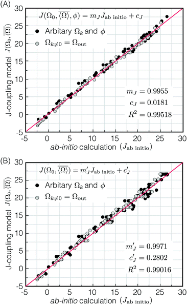 |
| | Fig. 9 (A) Plot comparing prediction of 2JSi–O–Si coupling model, eqn (17), and 2JSi–O–Si coupling from ab initio calculations. Gray and black dots correspond to 2JSi–O–Si couplings evaluated by systematic and arbitrary structural variations, respectively. The calculated Pearson correlation coefficient is R2 = 0.99518. (B) Plot comparing prediction of 2JSi–O–Si coupling model, eqn (19) and 2JSi–O–Si coupling from ab initio calculations. The calculated Pearson correlation coefficient is R2 = 0.99016. | |
Given that m2 ≪ m1 we find that the 2JSi–O–Si coupling model of eqn (17) can be simplified by dropping the m2cos3ϕ term to obtain
| |  | (19) |
A comparison of
ab initio2JSi–O–Si couplings with respect to the
2JSi–O–Si coupling model in
eqn (19) is presented in
Fig. 9B. Neglecting the
ϕ dependence leads to slightly greater scatter which is more noticeable at the higher couplings and a small drop of linear correlation coefficient to
R2 = 0.99016. Given this agreement all further analysis will use the
2JSi–O–Si coupling model of
eqn (19).
4.2 Mapping to local structure
Even with our approximate model for 2JSi–O–Si in eqn (19) being only a function of Ω0 and  there is no unique mapping of a single 2JSi–O–Si coupling back to local structure. Fortunately, the 29Si isotropic chemical shift of a Q4 site has a well established correlation7,9,43 to the mean inter-tetrahedral angle, 〈Ω〉, of a given Q4, of which, the linear correlation8is the simplest, while still giving a reasonably accurate correlation in the relevant range of 〈Ω〉 ∈ [140°,160°] as detailed further in the ESI.† The data for a number of crystalline silicas and siliceous framework silicates taken from the literature9,44,45 is shown in Fig. 10, along with a fit to eqn (20) with coefficients aδ and bδ provided in Table 1.
 |
| | Fig. 10 Linear correlation between average Si–O–Si bond angle, 〈Ω〉, about the Si tetrahedron and 29Si isotropic chemical shift, δCS. Twelve 29Si isotropic chemical shift sites in Tridymite were taken from Kitchin et al.45 and average Si–O–Si bond angles from Baur.44 The remaining were obtained from Engelhardt and Radeglia9 and references within. | |
Table 1 Final coefficients for eqn (22) after calibration with the results of Fig. 10 and eqn (23) after calibration with Sigma-2
| Coefficient |
Value |
Coefficient |
Value |
|
a
δ
|
−0.6148 ppm per ° |
b
δ
|
−19.297 ppm |
|
a
j
|
107.88° |
b
j
|
223.49° |
|
c
j
|
0.00002487° |
d
j
|
53.01 |
|
m
1
|
0.778 Hz per ° |
J
0
|
−7.5 Hz |
The 2JSi–O–Si coupling across 29Si(i)–O–29Si(j) linkage involves two 29Si isotropic chemical shifts, δCS,i and δCS,j, associated with 29Si(i) and 29Si(j) respectively. Using the linear correlation of eqn (20), the average 29Si isotropic chemical shift is given by
| |  | (21) |
With a simple inversion we have
| |  | (22) |
Inverting
eqn (19) for
Ω0 gives
| |  | (23) |
where the coefficient
aj,
bj,
cj and
dj are listed in
Table 1. Details on the solution for
Ω0 are given in Appendix A. To calibrate
eqn (23) against previous experimental measurements we use the
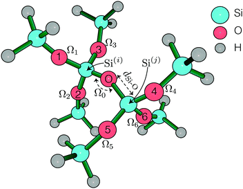
29Si INADEQUATE NMR results of Cadars
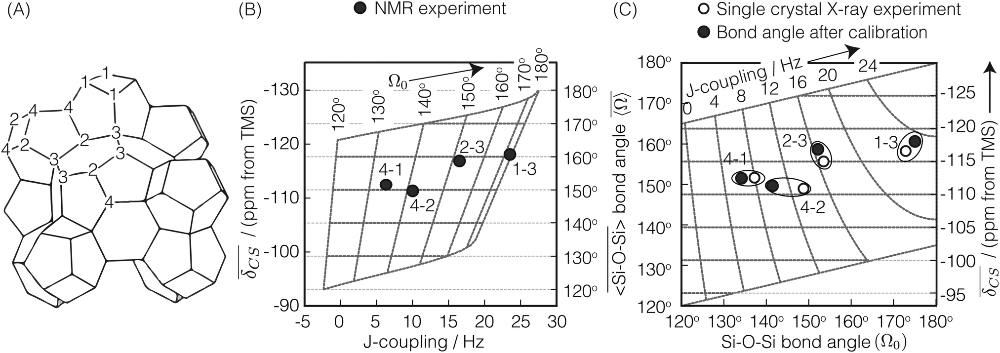
et al.26 on polycrystalline highly siliceous zeolite Sigma-2, whose structure, shown in
Fig. 11A, was predetermined using single crystal X-ray analysis. There are four observable
2JSi–O–Si couplings in Sigma-2. The observed
2JSi–O–Si coupling and the mean
29Si isotropic chemical shift,

, of the two coupled nuclei corresponding to the four
29Si–O–
29Si pairs from this measurement are listed in
Table 2. Here, the mean
29Si isotropic chemical shift,

, was determined as half the corresponding
29Si double quantum frequency of the INADEQUATE spectra. The X-ray determined Si–O–Si bond angle,
Ω0 and

, for these pairs are also listed in
Table 2. We choose to calibrate
eqn (23) by only varying
J0 to obtain agreement between model and experiment. This was accomplished by performing a least square minimization of the objective function
| |  | (24) |
where
Ω0(X-ray) is the Si–O–Si bond angle inferred from single crystal X-ray analysis, and
Ω0 is the Si–O–Si bond angle calculated using
eqn (23) with
m1 = 0.778 Hz per ° held constant. With this approach we obtain best agreement with
J0 = −7.5 ± 0.6 Hz.
 |
| | Fig. 11 (A) Schematic of highly siliceous zeolite Sigma-2 adapted from Cadars et al.26 (B) A correlation plot of  and J coupling for Sigma-2 with superimposed calibrated and J coupling for Sigma-2 with superimposed calibrated  and Ω0 grid. (C) Comparison of single crystal X-ray vs. NMR determined and Ω0 grid. (C) Comparison of single crystal X-ray vs. NMR determined  and Ω0 for the four different 29Si pairs in Sigma-2. Superimposed is the and Ω0 for the four different 29Si pairs in Sigma-2. Superimposed is the  and J coupling grid. A good agreement between the two results is observed for pair 4-1, 2-3 and 1-3. and J coupling grid. A good agreement between the two results is observed for pair 4-1, 2-3 and 1-3. | |
Table 2 Observed 2JSi–O–Si couplings (column 3) and 29Si average isotropic chemical shift,  , (column 2) for the 29Si pairs (column 1) in highly siliceous zeolite Sigma-2.26 Listed along column 4 and 5, is Ω0 and
  obtained from the crystal structure determined by single crystal X-ray analysis. Listed in column 6 and 7, is the Ω0 and
  calculated using eqn (22) and (23)
|
29Si pair |
Experimental |
Calculated |
| NMR |
Via X-ray |
Via NMR |
|

/ppm |
J/Hz |
Ω
0/° |

/° |
Ω
0/° |

/° |
| 1-3 |
−118.0 |
23.5 |
172.8 |
158.2 |
176.0 |
160.5 |
| 2-3 |
−116.8 |
16.5 |
153.5 |
155.6 |
152.0 |
158.6 |
| 4-2 |
−111.25 |
10.0 |
148.7 |
148.9 |
141.5 |
149.5 |
| 4-1 |
−112.4 |
6.3 |
137.2 |
151.6 |
134.0 |
151.4 |
A plot of measured 2JSi–O–Si coupling vs. from Sigma-2 is presented in Fig. 11B. Overlaid on top is a grid map of calibrated
  and Ω0. In Fig. 11C, the calculated
  and Ω0 (filled circles) along with X-ray determined
  and Ω0 (open circles) are presented. Overlaid on top is the grid map of J coupling and
  . Agreement to within ∼3° between Ω0 from the X-ray and NMR measurements is observed for pairs 4-1, 2-3 and 1-3, while there is a mismatch of ∼7° for the 4-2 pair. With only the limited data from Sigma-2, it is clear that additional experimental efforts in refinement of the calibration of eqn (23) would be helpful. Such efforts are, in fact, currently in progress in our laboratory on highly silicious zeolites using the recently developed PIETA method46 for rapid and sensitive 2D J NMR spectroscopy.
Overall, the results presented here are extremely promising and open the door to new opportunities to more fully exploit 2JSi–O–Si couplings as quantitative probes of structure in silicates. With only a ∼1 Hz change from the ab initio derived value of J0 = −8.3 ± 0.1 Hz, to the Sigma-2 calibrated value of J0 = −7.5 ± 0.6 Hz, the proposed correlated models of 29Si chemical shift and 2JSi–O–Si coupling provide an acceptable model for the quantitative interpretation of the 2JSi–O–Si coupling. It will be interesting to see if a similar analysis can be applied with other geminal J couplings across a bridging oxygen, such as a 31P–O–31P or 27Al–O–29Si linkage.
5 Summary
While both scalar J-couplings and homonuclear dipolar coupling are used qualitatively to establish connectivities between Si sites, it has been primarily homonuclear 29Si–29Si dipolar couplings through measurements of double quantum buildup curves that have provided some of the most useful quantitative details in the structure refinement of many siliceous zeolites and NMR crystallographic structural studies of meso- and microporous silicate materials.18,47,48 Here we have examined whether 2JSi−O−Si, the geminal coupling across a Si–O–Si linkage, can be turned into a more quantitative probe of the local structure in silicate networks.
Using high level density function theory (DFT) methods, we have found that the two main influences on the 2JSi–O–Si couplings are a primary dependence on the linkage Si–O–Si angle and a secondary dependence on mean Si–O–Si linkage of the two coupled 29Si nuclei. We show that the simple and highly approximate MO theory approach outlined by Pople and Santry35–40 can provide key insights when developing approximate models for geminal J-couplings based on results from high level density function theory (DFT) methods.25,26 Exploiting a well established correlation between 29Si isotropic chemical shift and the mean Si–O–Si angle of a Q4 site, we have developed an approach where a correlation plot of 2JSi–O–Si to mean 29Si isotropic chemical shift can be mapped into a 2D correlation of linkage Si–O–Si bond angle, Ω0, to mean Si–O–Si bond angle of the two coupled 29Si. Using available experimental 2JSi–O–Si couplings from Sigma-2,26 we found that only a minor adjustment of one ab initio derived coefficient in our 2JSi–O–Si model was needed to bring our model in line with experimental results.
Conflicts of interest
There are no conflicts to declare.
Appendix
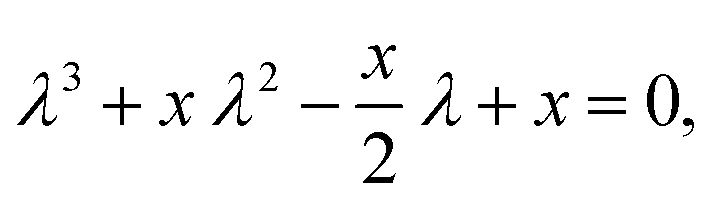
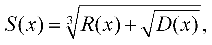
A Inversion of 2JSi–O–Si to Ω0
For inversion of eqn (19) with respect to Ω0, a close form solution can be obtained by first recasting eqn (19) into the form of a cubic equation| |  | (25) |
where λ = cosΩ0, and| |  | (26) |
The roots of eqn (25) are| |  | (27a) |
| |  | (27b) |
| |  | (27c) |
where we have defined| |  | (28a) |
| |  | (28b) |
| |  | (28c) |
| |  | (28d) |
The number of real and complex roots can be determined from the sign of the discriminant, D(x) in eqn (28d):
• If D(x) > 0, one root is real and two are complex conjugate.
• If D(x) = 0, all roots are real with at least two equal.
• If D(x) < 0, all roots are real and unequal.
For the given problem, the discriminant D(x), eqn (28d), is positive if x > −6.75. For given J0 < 0 Hz and m1 > 0° Hz−1, x is always positive and so is the discriminant. Therefore, there exists only one real root of eqn (25) given by eqn (27a). Thus, the inversion of eqn (19) with respect to Ω0 is
| |  | (29) |
To further simplify this result,
Ω0(
x) was approximated to a function
g(
x) that closely resembles
Ω0(
x) within the relevant range of 120° to 180°. For
Ω0(
x) ∈ [120°,180°],
λ1(
x) maps to a range
λ1(
x) ∈ [−0.5, −1.0] which further maps to a range
x ∈ [1/18,1/4]. Within the relevant range
x ∈ [1/18,1/4],
Ω0(
x) can be approximated as
| | | g(x) = aj + bjx + cjexp{djx}, | (30) |
where the coefficients are listed in
Table 1. The function
g(
x) provides a good approximation of
Ω0(
x) with |
g(
x) −
Ω0(
x)| < 0.5° within the range
Ω0(
x) ∈ [120°, 176°]. Deviations from 176° and onwards to a maximum of 3.7° at
Ω0(
x) = 180° is significant although can be neglected because of its low probability. A comparison of
Ω0(
x) and
g(
x) as a function of
x is provided in the ESI.
†
Acknowledgements
This material is based upon work supported by the National Science Foundation under Grant No. CHE-1506870.
References
-
G. Engelhardt and D. Michel, High-resolution solid-state NMR of silicates and zeolites, John Wiley & Sons, Chichester, 1987 Search PubMed.
-
C. A. Fyfe, Solid-State NMR for Chemists, C.F.C. Press, Guelph, 1983 Search PubMed.
-
K. J. D. Mackenzie and M. E. Smith, Multinuclear Solid-State NMR of Inorganic Materials, Pergamon, 2002 Search PubMed.
- N. Janes and E. Oldfield, J. Am. Chem. Soc., 1985, 107, 6769–6775 CrossRef CAS.
- J. F. Stebbins and B. T. Poe, Geophys. Res. Lett., 1999, 26, 2521–2523 CrossRef CAS.
- G. Engelhardt, H. Jancke, D. Hoebbel and W. Wieker, Z. Chem., 1974, 14, 109–110 CrossRef CAS.
- J. V. Smith and C. S. Blackwell, Nature, 1983, 303, 223–225 CrossRef CAS.
- J. Thomas, J. Klinowski, S. Ramdas, B. Hunter and D. Tennakoon, Chem. Phys. Lett., 1983, 102, 158–162 CrossRef CAS.
- G. Engelhardt and R. Radeglia, Chem. Phys. Lett., 1984, 108, 271–274 CrossRef CAS.
- A.-R. Grimmer, E. F. Gechner and G. Molgedey, Chem. Phys. Lett., 1981, 77, 331–335 CrossRef CAS.
- A.-R. Grimmer, Chem. Phys. Lett., 1985, 119, 416–420 CrossRef CAS.
- J. F. Stebbins, Nature, 1987, 330, 465 CrossRef CAS PubMed.
- P. Zhang, C. Dunlap, P. Florian, P. J. Grandinetti, I. Farnan and J. F. Stebbins, J. Non-Cryst. Solids, 1996, 204, 294–300 CrossRef CAS.
- P. Zhang, P. J. Grandinetti and J. F. Stebbins, J. Phys. Chem. B, 1997, 101, 4004–4008 CrossRef CAS.
- M. Davis, D. C. Kaseman, S. M. Parvani, K. J. Sanders, P. J. Grandinetti, P. Florian and D. Massiot, J. Phys. Chem. A, 2010, 114, 5503–5508 CrossRef CAS PubMed.
- M. Davis, K. J. Sanders, P. J. Grandinetti, S. J. Gaudio and S. Sen, J. Non-Cryst. Solids, 2011, 357, 2787–2795 CrossRef CAS.
- J. H. Baltisberger, P. Florian, E. G. Keeler, P. A. Phyo, K. J. Sanders and P. J. Grandinetti, J. Magn. Reson., 2016, 268, 95–106 CrossRef CAS PubMed.
- D. H. Brouwer, J. Am. Chem. Soc., 2008, 130, 6306–6307 CrossRef CAS PubMed.
- R. K. Harris and C. T. G. Knight, J. Chem. Soc., Faraday Trans. 2, 1983, 79, 1525–1538 RSC.
- R. K. Harris and C. T. G. Knight, J. Chem. Soc., Faraday Trans. 2, 1983, 79, 1539–1561 RSC.
- R. K. Harris, M. J. O'Connor, E. H. Curzon and O. W. Howarth, J. Magn. Reson., 1984, 57, 115–122 CAS.
- M. Haouas and F. Taulelle, J. Phys. Chem. B, 2006, 110, 3007–3014 CrossRef CAS PubMed.
- H. Cho, A. R. Felmy, R. Craciun, J. P. Keenum, N. Shah and D. A. Dixon, J. Am. Chem. Soc., 2006, 128, 2324–2335 CrossRef CAS PubMed.
- S. Cadars, A. Lesage, N. Hedin, B. F. Chmelka and L. Emsley, J. Phys. Chem. B, 2006, 110, 16982–16991 CrossRef CAS PubMed.
- P. Florian, F. Fayon and D. Massiot, J. Phys. Chem. C, 2009, 113, 2562–2572 CAS.
- S. Cadars, D. H. Brouwer and B. F. Chmelka, Phys. Chem. Chem. Phys., 2009, 11, 1825–1837 RSC.
- J. Autschbach and B. Le Guennic, J. Chem. Educ., 2007, 84, 156 CrossRef CAS.
-
M. J. Frisch, G. W. Trucks, H. B. Schlegel, G. E. Scuseria, M. A. Robb, J. R. Cheeseman, G. Scalmani, V. Barone, B. Mennucci, G. A. Petersson, H. Nakatsuji, M. Caricato, X. Li, H. P. Hratchian, A. F. Izmaylov, J. Bloino, G. Zheng, J. L. Sonnenberg, M. Hada, M. Ehara, K. Toyota, R. Fukuda, J. Hasegawa, M. Ishida, T. Nakajima, Y. Honda, O. Kitao, H. Nakai, T. Vreven, J. A. M. Jr., J. E. Peralta, F. Ogliaro, M. J. Bearpark, J. J. Heyd, E. N. Brothers, K. N. Kudin, V. N. Staroverov, T. A. Keith, R. Kobayashi, J. Normand, K. Raghavachari, A. P. Rendell, J. C. Burant, S. S. Iyengar, J. Tomasi, M. Cossi, N. Rega, J. M. Millam, M. Klene, J. E. Knox, J. B. Cross, V. Bakken, C. Adamo, J. Jaramillo, R. Gomperts, R. E. Stratmann, O. Yazyev, A. J. Austin, R. Cammi, C. Pomelli, J. W. Ochterski, R. L. Martin, K. Morokuma, V. G. Zakrzewski, G. A. Voth, P. Salvador, J. J. Dannenberg, S. Dapprich, A. D. Daniels, O. Farkas, J. B. Foresman, J. V. Ortiz, J. Cioslowski and D. J. Fox, Gaussian 09 Revision D.01, 2013 Search PubMed.
-
O. S. Center, Ohio Supercomputer Center, 1987 Search PubMed.
-
E. D. Glendening, A. E. Reed, J. E. Carpenter and F. Weinhold, NBO Version3.1, 1988 Search PubMed.
- S. van der Walt, S. C. Colbert and G. Varoquaux, Comput. Sci. Eng., 2011, 13, 22–30 CrossRef.
-
M. Newville, T. Stensitzki, D. B. Allen and A. Ingargiola, LMFIT: Non-Linear Least-Square Minimization and Curve-Fitting for Python, 2014 Search PubMed.
- J. D. Hunter, Comput. Sci. Eng., 2007, 9, 90–95 CrossRef.
- P. J. Grandinetti, J. T. Ash and N. M. Trease, Prog. Nucl. Magn. Reson. Spectrosc., 2011, 59, 121–196 CrossRef CAS PubMed.
- J. Pople and D. Santry, Mol. Phys., 1964, 7, 269–286 CrossRef CAS.
- J. Pople and D. Santry, Mol. Phys., 1964, 8, 1–18 CrossRef CAS.
- J. Pople and D. Santry, Mol. Physiol., 1965, 9, 311–318 CrossRef CAS.
- J. Pople and D. Santry, Mol. Phys., 1965, 9, 301–310 CrossRef CAS.
- J. A. Pople, D. P. Santry and G. A. Segal, J. Chem. Phys., 1965, 43, S129–S135 CrossRef CAS.
- M. Barfield, Magn. Reson. Chem., 2007, 45, 634–646 CrossRef CAS PubMed.
- C. A. Coulson and H. C. Longuet-Higgins, Proc. R. Soc. London, Ser. A, 1947, 191, 39–60 CrossRef CAS.
-
M. Klessinger and M. Barfield, The structural dependence of geminal 13C–13C coupling constants, Ellis Horwood, Chichester, 1987, ch. 16, pp. 269–284 Search PubMed.
- F. Mauri, A. Pasquarello, B. G. Pfrommer, Y.-G. Yoon and S. G. Louie, Phys. Rev. B: Condens. Matter Mater. Phys., 2000, 62, 4786–4789 CrossRef.
- W. H. Baur, Acta Crystallogr., Sect. B: Struct. Crystallogr. Cryst. Chem., 1977, 33, 2615–2619 CrossRef.
- S. J. Kitchin, S. C. Kohn, R. Dupree, C. M. B. Henderson and K. Kihara, Am. Mineral., 1996, 81, 550–560 CAS.
- J. H. Baltisberger, B. J. Walder, E. G. Keeler, D. C. Kaseman, K. J. Sanders and P. J. Grandinetti, J. Chem. Phys., 2012, 136, 211104 CrossRef PubMed.
- D. H. Brouwer, S. Cadars, J. Eckert, Z. Liu, O. Terasaki and B. F. Chmelka, J. Am. Chem. Soc., 2013, 135, 5641–5655 CrossRef CAS PubMed.
- D. H. Brouwer, Solid-State NMR Spectrosc., 2013, 51–52, 37–45 CrossRef CAS PubMed.
Footnote |
| † Electronic supplementary information (ESI) available. See DOI: 10.1039/c7cp06486a |
|
| This journal is © the Owner Societies 2018 |
Click here to see how this site uses Cookies. View our privacy policy here. 
 *a
*a


 , (B) O–Si–Si–O inter tetrahedral dihedral angle, ϕ and (C) Si–O bond distance, dSi–O. For calculations in (A) dSi–O = 1.60 Å and Ωk≠0 = Ωout varied from 120° to 180°. In (B) dSi–O = 1.60 Å, Ωout = 146° and ϕ varied from −60° to +60°. In (C) Ωout = 146° and d varied from 1.58 Å to 1.62 Å.

 we show (vide infra) that a combined measurement of isotropic 29Si chemical shift and 2JSi–O–Si can be exploited to determine the local structure around the Q4–Q4 linkage.
 in eqn (2), with the exception of the singular—and highly unlikely—occurrence of
  . To ensure a systematic variation of the local structure, we choose to constrain all Ωk≠0 = Ωout. A series of 2JSi–O–Si calculations were performed by independently vary Ωout and Ω0 from 120° to 180° on a uniform grid. The calculated 2JSi–O–Si as a function of
  and Ω0 is presented in Fig. 2A. All Si–O bond distances were set to 1.6 Å. Of course, the constraint Ωk≠0 = Ωout, implemented only to ensure a systematic local structural variation, is unrealistic even for most crystalline silicates and highly siliceous zeolites, as well as in silica glass and other silica rich disordered materials. To break free from this constraint numerous 2JSi–O–Si coupling calculations were performed at arbitrary outer Si–O–Si bond angles Ωk≠0 and ϕ, with values listed in Tables S3 and S4 of the ESI.† These calculations are used to further verify agreement with our proposed 2JSi–O–Si coupling model.


 are ignored, the mutual atom–atom polarizability term can be approximated42 to
 and
and  are the products of the s-character of the valence HTOs associated with the Si(i)–O and Si(j)–O bonds across Si(i)–O–Si(j) linkage, respectively, as illustrated in Fig. 3.
 , and
, and  at the bridging oxygen and adjacent silicons respectively. These values were determined from the quantum chemistry DFT cluster calculation using Gaussian NBO version 3.1. For clarity, we only present a subset of results from Fig. 2 per structural parameters considered.
 , as predicted by eqn (14). As noted earlier, the slight deviation from linearity observed is not unexpected and is likely attributed to the neglected terms in the mutual atom–atom polarizability term. In Fig. 4C and D we see that the variation in 2JSi–O–Si primarily arises from variation in a4O,—the s-character product of the two valence HTOs at the bridging oxygen—while there is a minor yet non-negligible variation coming from
  —the s-character product of the two silicon valence HTOs in the Si–O–Si linkage. The change in a4O is the result of the change in the hybridization of the valence orbitals at the bridging oxygen from sp2 (33.33% s-character) at Ω0 = 120° to sp (50% s-character) at Ω0 = 180°. A popular approximation for the s-character at the bridging oxygen9,42 is given by

 , (C) a4O, and (D)
  for the constraints Ωk≠0 = 180° and d = 1.6 Å.
 is also as expected at ∼(25%)2 = 6.25%. The slight increase in
  from 6.1% to 6.7% in Fig. 4D with decreasing Ω0 may seem surprising from a simple hybrid orbital picture—as all intra-tetrahedral angles and Si–O distances are held constant at ∠O−Si−O = 109.5° and dSi–O = 1.6 Å, respectively, in these calculations. In fact, for this subset of results, even the outer Si–O–Si angles are held fixed at 180°, so it is only the variation of the linkage angle Ω0 that is responsible for this slight change in
  . We will examine the origin of this variation shortly when the influence of the outer Si–O–Si angles on 2JSi–O–Si are considered.
 , and in Fig. 5C we see no observable dependence of 2JSi–O–Si coupling on the s-character product a4O at the bridging oxygen. This is because, for this subset of calculations, the hybridization at the bridging oxygen was locked to sp through the constraint Ω0 = 180°. Since the s-character at the bridging oxygen predominantly depends on the Si–O–Si bond angle, as noted in eqn (15), the change in Si–O bond distance, dSi–O, shows no observable change in its s-character. In Fig. 5D we find that the minor variation in 2JSi–O–Si coupling is dominated by the change in
  . While a decrease in the a2Si with increasing Si–O bond distance has been previously reported by Grimmer and coworkers10,11 it was in the context of correlated changes in the intra-tetrahedral angle ∠O–Si–O. With the intra-tetrahedral angles in this calculation fixed at ∠O–Si–O = 109.5°, it seems that changes in Si–O length alone lead to minor variations in a2Si—although these result in relatively insignificant variations in 2JSi–O–Si.
 , (C) a4O, and (D)
  for the constraints Ω0 = 180° and Ωk≠0 = 146°.
 , (C) a4O, and (D)
  for the constraints Ωk≠0 = 146°, Ω0 = 180° and d = 1.6 Å.
 , as calculated by eqn (2), for a subset of results from Fig. 2A subjected to the constraint Ω0 = 180°, Ωk≠0 = Ωout and d = 1.6 Å where Ωout varied from 120° to 180°. The variation in Fig. 7A is about 25% of that shown in Fig. 4A and is found to be the second most dominant dependence of 2JSi–O–Si coupling. As Ω0 is fixed, it is the change in the outer Si–O–Si bond angles, Ωout, that leads to this variation in 2JSi–O–Si. In Fig. 7B we again find the markedly linear correlation of 2JSi–O–Si coupling with
  as predicted by eqn (14). As might be expected, no observable dependence of 2JSi–O–Si coupling on a4O is observed in Fig. 7C since the hybridization at the bridging oxygen was fixed to sp with the constraint Ω0 = 180°.
 , (B)
, (B)  , (C) a4O, and (D)
  for the constraints Ω0 = 180° and d = 1.6 Å.
 as seen in Fig. 7D. Why would the
  or
or  increase as the outer angles, Ωout, increase? This is the same question alluded to earlier with respect to Fig. 4D. The logic is as follows. We expect the sum of the s-characters for the four HTO around each silicon to be constant. So, as the s-character of one HTO deviates from 25%, the s-characters of the other HTO compensate to maintain the constant sum. Hence, we expect the s-character of the HTO that is part of the central linkage to increase as the average s-character of the other three HTOs decreases. Close examination of the variation in
  as the function of the Si–O–Si tetrahedral angle, Ω0, and average Si–O–Si bond angle, 〈Ω〉i, also shown in Fig. S3 of the ESI,† reveals an approximate proportionality given by
 , decreases as Ω0 increases.
 . From the ab initio calculations, shown in Fig. 8, however, we find that the 2JSi–O–Si coupling is better described by a quadratic in the s-character product,
  , with R2 = 0.99164. As mentioned earlier, this slight curvature is not unexpected, since the model in eqn (14) neglects all the vicinal integrals from the mutual atom–atom polarizability term. Further discussion on the effect of vicinal integrals can be found in the chapter by Klessinger and Barfield.42
 at Si(i), Si(j) and O across Si(i)–O–Si(j) linkage. The points in gray and black corresponds to the systematic (Ωk≠0 = Ωout) and arbitrary structural variations, respectively.
 , for both systematic and arbitrary structural variation.


 there is no unique mapping of a single 2JSi–O–Si coupling back to local structure. Fortunately, the 29Si isotropic chemical shift of a Q4 site has a well established correlation7,9,43 to the mean inter-tetrahedral angle, 〈Ω〉, of a given Q4, of which, the linear correlation8


 , of the two coupled nuclei corresponding to the four 29Si–O–29Si pairs from this measurement are listed in Table 2. Here, the mean 29Si isotropic chemical shift,
  , was determined as half the corresponding 29Si double quantum frequency of the INADEQUATE spectra. The X-ray determined Si–O–Si bond angle, Ω0 and
  , for these pairs are also listed in Table 2. We choose to calibrate eqn (23) by only varying J0 to obtain agreement between model and experiment. This was accomplished by performing a least square minimization of the objective function
 and J coupling for Sigma-2 with superimposed calibrated
  and Ω0 grid. (C) Comparison of single crystal X-ray vs. NMR determined
  and Ω0 for the four different 29Si pairs in Sigma-2. Superimposed is the
  and J coupling grid. A good agreement between the two results is observed for pair 4-1, 2-3 and 1-3.
 , (column 2) for the 29Si pairs (column 1) in highly siliceous zeolite Sigma-2.26 Listed along column 4 and 5, is Ω0 and
  obtained from the crystal structure determined by single crystal X-ray analysis. Listed in column 6 and 7, is the Ω0 and
  calculated using eqn (22) and (23)


 from Sigma-2 is presented in Fig. 11B. Overlaid on top is a grid map of calibrated
  and Ω0. In Fig. 11C, the calculated
  and Ω0 (filled circles) along with X-ray determined
  and Ω0 (open circles) are presented. Overlaid on top is the grid map of J coupling and
  . Agreement to within ∼3° between Ω0 from the X-ray and NMR measurements is observed for pairs 4-1, 2-3 and 1-3, while there is a mismatch of ∼7° for the 4-2 pair. With only the limited data from Sigma-2, it is clear that additional experimental efforts in refinement of the calibration of eqn (23) would be helpful. Such efforts are, in fact, currently in progress in our laboratory on highly silicious zeolites using the recently developed PIETA method46 for rapid and sensitive 2D J NMR spectroscopy.