Axial–equatorial isomerism and semiexperimental equilibrium structures of fluorocyclohexane

Abstract

An experimental-computational methodology combining rotational data, high-level ab initio calculations and predicate least-squares fitting is applied to the axial–equatorial isomerism and semiexperimental equilibrium structure determination of fluorocyclohexane. New supersonic-jet microwave measurements of the rotational spectra of the two molecular conformations, together with all ¹³C isotopologues of both isomeric forms are reported. Equilibrium rotational constants are obtained from the ground-state rotational constants corrected for vibration–rotation interactions and electronic contributions. Equilibrium structures were determined by the mixed estimation (ME) method. Different computational methods were tested for the evaluation of predicate values of the structural parameters, and a computationally effective procedure for estimating reliable dihedral angles is proposed. Structural parameters were fitted concurrently to predicate parameters and moments of inertia, affected with appropriate uncertainties. The new structures of the title compound are regarded as accurate to 0.001 Å and 0.2°, illustrating the advantages of this methodology. Structural comparisons are offered with the cyclohexane prototype, revealing subtle substituent effects. For comparison purposes the equilibrium structures for the two fluorocyclohexane isomers and cyclohexanone are computed from high-level ab initio theory with inclusion of adjustments for basis set dependence and correlation of the core electrons.

---

Introduction

The semiexperimental (SE) method is an experimental-computational procedure where equilibrium rotational constants are determined from the experimental ground-state rotational constants and theoretical rovibrational corrections (based principally on an ab initio cubic force field). Since the pioneering work of Pulay et al.¹ the SE method is reputed to deliver very accurate estimates to equilibrium structures² of (mostly) semirigid molecules of small and medium molecular sizes,^3–6 reaching bond length accuracy to about 0.001 Å, and similar four-digit accurate values for bond angles. However, difficulties for the application of the SE method increase rapidly with the molecular size. From the experimental point of view, determination of rotational parameters for full sets of isotopologues is hampered by spectral congestion and weak intensities due to larger rotational partition functions, distributing the rotational energy among a larger number of states. Moreover, it was observed that, in some cases, the rotational constants of deuterated species do not improve the fits.⁷ Furthermore, the system of normal equations of the least-squares method may easily become ill-conditioned (i.e. sensitive to small errors of the input data), in particular for atoms close to the center of mass (in other words, their isotopic substitution does not bring new information).

These difficulties may be circumvented by the use of the predicate observations or mixed estimation (ME) method,^8,9 where auxiliary information called predicates is added with appropriate weights to the data matrix during the least-squares fit.¹⁰ Estimates of the predicates (bond lengths and bond angles) are generally (but not necessarily) obtained from quantum chemical (QC) calculations at an accessible level of theory, eventually improved by corrections based on comparisons between QC predictions and known equilibrium structures for various types of chemical bonds. An important advantage of the mixed estimation method is that no specific constraints are introduced, which avoids biased results. The determination of the predicates for different organic molecules has already been discussed.¹¹ It is easy to obtain reliable predicates for the CH bond lengths, the single CC bond lengths and related bond angles. However, as observed in fructose,¹² deoxyribose,¹² proline,¹³ succinic anhydrid,¹⁴ pseudopelletierine¹⁵ and several other molecules the prediction of accurate dihedral angles is a problem, the error being sometimes as large as several degrees. Indeed, a provisional criticism of the ME method is the difficulty to obtain reliable estimates for a full set of internal coordinates and to simultaneously estimate their accuracy. In this paper, we plan to study two aspects of this problem: (1) how to obtain predicates of the CF bond lengths and of dihedral angles and (2) how to achieve computational accuracy without having recourse to expensive methods such as the coupled–cluster methods. Then, these results will be applied to the determination of the semiexperimental structure of the axial and equatorial conformers of fluorocyclohexane. Fluorocyclohexane is an appropriate candidate to compare the small structural and energetic effects caused by axial/equatorial substituents in the canonical cyclohexane chair. Moreover, the small conformational energies between the axial and equatorial forms anticipate the possibility of detecting all ¹³C isotopologues in natural abundance for both species, improving the empirical data for the structural analysis. The structure of cyclohexanone was additionally optimized ab initio to compare with fluorocyclohexane and in order to have a larger variety of torsional angles.

The first study of the structure of fluorocyclohexane by Andersen in 1962 used gas-phase electron diffraction.¹⁶ He determined the ratio between the axial and equatorial conformations and found that the conformation with fluorine in equatorial position is more stable by about 170 cal mol⁻¹. Slightly later, the microwave spectra of both forms were analyzed by Pierce et al.^17,18 In 1971 Scharpen measured the relative intensities of rotational transitions of both conformers and determined an energy difference of 259(28) cal mol⁻¹.¹⁹ Empirical structures for both conformers were independently determined more recently by Bialkowska-Jaworska et al.²⁰ and Durig et al.²¹ The latter authors also determined an accurate value of the enthalpy difference, ΔH = 137(14) cal mol⁻¹ from the analysis of the infrared spectra in gas and xenon solution. The intensities of several well-isolated and well-shaped conformational bands were measured as a function of temperature (at 5.0 °C intervals between −60 and −100 °C) and ΔH was determined by application of the van’t Hoff equation assuming that the conformational enthalpy differences are not a function of temperature in the range studied. The conformational equilibria were also studied theoretically by Storz.²²

Experimental and computational methods

The jet-cooled rotational spectrum of fluorocyclohexane was measured in the frequency range 6–20 GHz with a Fourier transform microwave (FT-MW) spectrometer based on the Balle-Flygare²³ design. The sample was vaporized on an external liquid reservoir inserted in the carrier gas line (ice temperature). A stream of argon (backing pressures ca. 1 bar) was flowed over the sample and expanded through a solenoid valve (Parker, nozzle diameter 1.0 mm), creating a pulsed supersonic jet. The jet was probed within a Fabry–Perot microwave resonator, formed by two spherical mirrors in near confocal position (diameter 33 cm). The injection valve was located near the center of one of the mirrors, resulting in a collinear arrangement of the jet and resonator axis.²⁴ The gas pulses (∼500 μs) expanding the vaporized sample were followed by short microwave impulses (∼1 μs, <100 mW), polarizing the polar molecules. Up to 4 microwave pulses were used per gas pulse. The emitted free-induction decay was recorded in the time-domain (410 μs), amplified and recorded with a heterodyne receiver centered at 30 MHz. The digital signal was processed with the FTMW++ program developed at the Leibniz Universität Hannover.²⁴ Typically, hundreds/thousands of experiments were coadded in the time domain for signal averaging. All frequency oscillators in the system were locked to a rubidium standard, providing frequency accuracies of the rotational transitions below 5 kHz. Line transitions appear as Doppler doublets, so the rest frequencies were taken from the averaged frequencies.

Different ab initio calculations were required for this work. The geometry optimizations were performed at the level of coupled-cluster method²⁵ with a perturbative treatment of connected triples²⁶ (CCSD(T)) using the cc-pwCVTZ basis set,²⁷ all electrons being correlated (AE). The second-order Møller–Plesset perturbation theory (MP2)²⁸ was also used at the frozen-core (FC) and all-electron (AE) levels using different basis sets: cc-pVTZ,²⁹ 6-311+G(3df,2pd),³⁰ cc-pwCVTZ and cc-pwCVQZ.²⁷ The density functional theory (B3LYP)^31–33 was also employed with the 6-311+G(3df,2pd) basis set. In order to determine the rovibrational contributions to the rotational constants, the anharmonic force field up to semidiagonal quartic terms was calculated at the MP2_FC/cc-pVTZ level of theory.³⁴ This calculation was repeated for each isotopologue, as different isotopes require distinct vibrational corrections. To avoid the nonzero force field dilemma,³⁵ all force fields were evaluated at the corresponding optimized geometries. The MP2 and B3LYP calculations were performed with the Gaussian 09 package (Rev. A.02 or C.01),³⁶ whereas the MolPro program³⁷ was used for the CCSD(T) calculations. The charges on the atoms were calculated using the Atoms in Molecules (AIM) theory³⁸ with its implementation in Gaussian03 by Cioslowski et al.³⁹ The calculations were performed at the B3LYP/6-311+G(3df,2pd) level of theory at the equilibrium structure.

Results

1. Rotational spectra

We first measured and analyzed the rotational spectra for the parent isotopologue (¹²C) of both axial and equatorial conformers, extending previous experiments. Later on, we could assign all monosubstituted ¹³C isotopologues in natural abundance (ca. 1%) for the two conformers, as illustrated in Fig. 1. A centrifugal-distorted rotational Hamiltonian complete up to quartic terms in the asymmetric-top reduction and the I^r representation was used to fit the spectra.⁴⁰ The quality of the structural fit is very sensitive to the true accuracy of the ground-state rotational constants.^41,42 As the small number of transitions and their low angular momentum quantum numbers (J = 1–6) did not permit to obtain a full set of meaningful centrifugal distortion constants, the mixed regression method was used.⁹ The experimental frequencies were fitted together with appropriately weighted ab initio (predicate) values for the centrifugal distortion constants. The predicate constants were obtained from a harmonic force field calculated at the MP2_FC/cc-pVTZ level, the uncertainty used to determine their weight being 10% of their value. The experimental rotational frequencies are given in Tables S1–S10 (ESI†) and the derived rotational constants are collected in Tables 1 and 2. It is worth noting that the centrifugal distortion effects are larger in the axial form.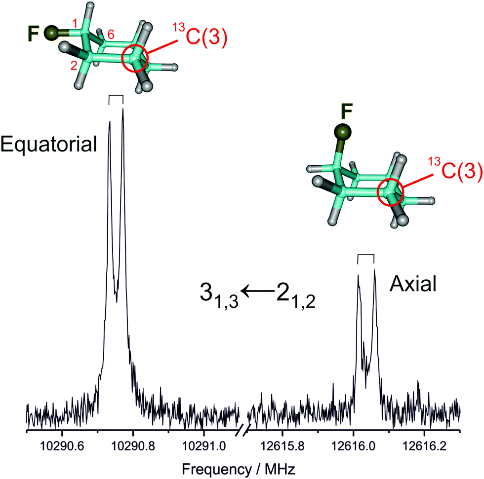

Fig. 1 A typical rotational transition corresponding to one of the ¹³C monosubstituted isotopologues of equatorial and axial fluorocyclohexane, measured in natural abundance.

Table 1 Experimental rotational parameters for the equatorial conformer of fluorocyclohexane

	Parent	^13C(1)	^13C(2)	^13C(3)	^13C(4)
a Rotational constants (A, B, C), centrifugal distortion constants (ΔJ, ΔJK, ΔK, δJ, δK), number of fitted transitions (N) and rms deviation of the fit (σ). b Standard errors in parentheses in units of the last digit.
A /MHz	4313.36670(41)^b	4309.5918(14)	4255.1484(33)	4255.0763(12)	4310.5763(18)
B/MHz	2188.78913(17)	2179.702324(51)	2187.94976(13)	2174.164386(46)	2153.373068(66)
C/MHz	1591.61099(11)	1587.368270(50)	1583.48471(10)	1576.365987(36)	1573.224557(53)
Δ J/kHz	0.13231(42)	0.131836(85)	0.13161(23)	0.129916(77)	0.12958(11)
Δ JK/kHz	0.12551(40)	0.120431(77)	0.12367(22)	0.128700(76)	0.113250(97)
Δ K/kHz	0.6283(20)	0.63016(40)	0.6128(11)	0.60836(36)	0.64220(55)
δ J/kHz	0.03511(11)	0.034951(22)	0.035284(63)	0.034637(21)	0.034137(29)
δ K/kHz	0.25114(81)	0.24999(16)	0.24702(44)	0.24760(15)	0.24672(21)
N	30	8	12	10	9
σ/kHz	54.9	1.7	1.7	1.7	1.8

---

Table 2 Experimental rotational parameters for the axial conformer of fluorocyclohexane

	Parent	^13C(1)	^13C(2)	^13C(3)	^13C(4)
a Rotational constants (A, B, C), centrifugal distortion constants (ΔJ, ΔJK, ΔK, δJ, δK), number of fitted transitions (N) and rms deviation of the fit (σ). b Standard errors in parentheses in units of the last digit.
A /MHz	3562.96908(16)^b	3557.1443(26)	3513.75817(37)	3522.20266(13)	3562.82765(62)
B/MHz	2628.624997(95)	2609.74750(24)	2622.57510(28)	2614.58544(10)	2584.80434(12)
C/MHz	1980.88163(11)	1972.02062(24)	1968.11042(22)	1961.731079(86)	1956.016082(83)
Δ J/kHz	0.5543(35)	0.5353(60)	0.5515(66)	0.5499(26)	0.5398(18)
Δ JK/kHz	−1.043(12)	−1.019(16)	−1.019(19)	−1.0185(65)	−1.0307(36)
Δ K/kHz	1.285(15)	1.263(20)	1.253(23)	1.2453(80)	1.2873(45)
δ J/kHz	0.0877(10)	0.0849(13)	0.0861(15)	0.08896(57)	0.0947(20)
δ K/kHz	0.0854(10)	0.0792(12)	0.0831(15)	0.08676(56)	0.08158(28)
N	32	6	7	7	6
σ/kHz	26.1	0.93	0.89	1.3	1.09

---

2. Equilibrium structures

The Born–Oppenheimer (BO) equilibrium structures were optimized at the CCSD(T)_AE/cc-pwCVTZ level of theory for the equatorial and axial conformers of fluorocyclohexane. The small effect of further basis set enlargement (cc-pwCVTZ → cc-pwCVQZ) was then estimated at the MP2 level. The resulting estimate was:

r^BO_e = r_e[CCSD(T)_AE/cc-pwCVTZ] + r_e[MP2_AE/cc-pwCVQZ] + r_e[MP2_AE/cc-pwCVTZ] (1)

The accuracy of this equation, which is based on the additivity of small corrections, was confirmed many times, see for instance ref. 42–45. The BO structure of equatorial cyclohexanone was computed similarly (see Table S11, ESI†) with details of the calculations given in Table S12 (ESI†). The BO structures of equatorial and axial conformers of fluorocyclohexane are presented in Tables 3 and 4, respectively, and the details of the calculations are given in Tables S13 and S14 (ESI†).

Table 3 Equilibrium structure of equatorial fluorocyclohexane (distances in Å and angles in degree)

Method Basis set	MP2_FC/cc-pVTZ	B3LYP/6-311+^a	r ^SEe	r ^BOe
a 6-311+G(3df,2pd). b Estimated according to eqn (1) (see text).
C1C2	1.5125	1.5189	1.51218(43)	1.5131
C2C3	1.5276	1.5347	1.53121(71)	1.5282
C3C4	1.5260	1.5324	1.52554(25)	1.5262
C1Fq	1.3954	1.4063	1.39260(62)	1.3945
C1Ha	1.0940	1.0945	1.0942(15)	1.0939
C2Hq	1.0899	1.0910	1.0893(24)	1.0900
C2Ha	1.0925	1.0935	1.0934(15)	1.0930
C3Hq	1.0900	1.0912	1.0892(22)	1.0901
C3Ha	1.0937	1.0947	1.0946(13)	1.0941
C4Hq	1.0906	1.0918	1.0905(17)	1.0907
C4Ha	1.0934	1.0945	1.0941(15)	1.0939
C1C2C3	110.19	110.66	110.168(32)	110.24
C2C3C4	110.90	111.50	111.007(21)	111.02
C3C4C5	110.78	111.43	110.982(22)	110.97
C2C1C6	111.73	112.36	112.007(36)	111.96
FqC1C2	109.28	109.17	109.084(30)	109.17
FqC1Ha	106.69	105.77	106.51(15)	106.51
C1C2Hq	109.60	109.63	109.50(15)	109.59
C1C2Ha	108.16	108.29	108.01(20)	108.16
C2C3Hq	109.94	109.70	109.84(15)	109.87
C2C3Ha	109.38	109.39	109.03(25)	109.34
C3C4Hq	110.32	110.15	110.246(74)	110.26
C3C4Ha	109.17	109.21	109.121(75)	109.14
HqC2Ha	107.60	107.21	107.53(28)	107.61
HqC3Ha	106.73	106.34	107.07(23)	106.73
HqC4Ha	107.00	106.57	107.03(21)	106.97
C1C2C3C4	56.36	54.76	55.990(51)	55.97
FqC1C2C3	−178.55	−177.38	−178.154(37)	−178.18
FqC1C2Hq	58.71	59.88	59.05(19)	59.11
FqC1C2Ha	−58.33	−56.78	−57.77(30)	−57.93
C1C2C3Hq	179.07	177.48	178.57(16)	178.64
C1C2C3Ha	−64.05	−66.24	−64.40(14)	−64.53
C2C3C4Hq	−178.51	−176.90	−178.20(14)	−178.20
C2C3C4Ha	64.18	66.39	64.53(13)	64.58

---

Table 4 Equilibrium structure of axial fluorocyclohexane (distances in Å and angles in degree)

Method Basis set	MP2_FC/cc-pVTZ	B3LYP/6-311+^a	r ^SEe	r ^BOe
a 6-311+G(3df,2pd). b Estimated according to eqn (1) (see text).
C1C2	1.5159	1.5218	1.51423(94)	1.5162
C2C3	1.5259	1.5326	1.5257(13)	1.5265
C3C4	1.5260	1.5323	1.52690(71)	1.5261
C1Fa	1.4015	1.4134	1.4036(13)	1.4013
C1Hq	1.0909	1.0921	1.0908(25)	1.0908
C2Hq	1.0901	1.0912	1.0901(27)	1.0902
C2Ha	1.0932	1.0945	1.0938(32)	1.0937
C3Hq	1.0903	1.0916	1.0902(24)	1.0905
C3Ha	1.0915	1.0924	1.0921(38)	1.0919
C4Hq	1.0906	1.0918	1.0905(46)	1.0907
C4Ha	1.0944	1.0955	1.0949(39)	1.0949
C1C2C3	111.40	112.21	111.605(57)	111.62
C2C3C4	110.84	111.47	110.942(77)	110.96
C3C4C5	110.62	111.27	110.618(53)	110.79
C2C1C6	112.37	112.98	112.729(76)	112.61
C2C1Hq	110.71	110.67	110.667(80)	110.71
FaC1Hq	106.31	105.52	106.14(14)	106.15
C1C2Hq	109.03	108.99	109.04(17)	109.02
C1C2Ha	107.90	107.65	107.56(22)	107.74
C2C3Hq	109.86	109.69	109.72(20)	109.78
C2C3Ha	109.01	109.05	108.77(34)	109.05
C3C4Hq	110.32	110.12	110.27(14)	110.26
C3C4Ha	109.30	109.36	109.30(13)	109.28
HqC2Ha	107.38	106.86	107.21(32)	107.36
HqC3Ha	107.10	106.68	107.27(34)	107.09
HqC4Ha	106.91	106.49	107.00(33)	106.89
C1C2C3C4	55.20	53.25	54.72(10)	54.66
C3C2C1Hq	−178.14	−176.30	−177.53(13)	−177.57
HqC1C2Hq	58.88	60.31	59.28(28)	59.31
HqC1C2Ha	−57.44	−55.25	−56.66(34)	−56.89
C1C2C3Hq	177.79	175.92	177.15(20)	177.20
C1C2C3Ha	−65.13	−67.59	−65.79(18)	−65.76
C2C3C4Hq	−179.36	−177.64	−179.12(24)	−179.07
C2C3C4Ha	63.36	65.68	63.52(21)	63.73

---

3. Determination of structural predicates

For the determination of the predicates, the MP2_FC/cc-pVTZ level of theory generally gives satisfactory results for the CH bond lengths, the single CC bond lengths and the bond angles.¹¹ The accuracy is about 0.002 Å for the CH bonds and slightly better than 0.003 Å for the CC bonds. For the bond angles, the MP2_FC/6-311+G(3df,2pd) method gives slightly better results than MP2_FC/cc-pVTZ, the accuracy of the former being better than 0.3° in most cases instead of 0.4° for the latter.¹² It is worth noting that, for large molecules, it may be advantageous to use DFT methods such as B3LYP or B2PLYP.^46,47 This choice is at first sight somewhat arbitrary because there are many functionals and many basis sets available. However, the B3LYP method is broadly used and is known to give accurate results with the split-valence 6-311+G(3df,2pd) basis set.⁴⁸

a. Predicates for the dihedral angles. To determine the position of the hydrogen atoms, the knowledge of the dihedral angles τ(CCCH) or τ(HCCH) is necessary. However, they cannot be obtained from the rotational constants because the rotational spectra of the deuterated species have not been analyzed. In principle, it would be possible to synthesize all the monodeuterated species and to measure their rotational spectra but it would be difficult and extremely time-consuming. Furthermore, the rotational constants of the deuterated species have sometimes large systematic errors because of the large mass increase.⁷ For these reasons, it is important to have reliable predicates for these torsional angles.

As observed in fructose, deoxyribose,¹² and pseudopelletierine,¹⁵ the MP2 method fails to deliver accurate dihedral angles, the error being sometimes as large as several degrees. This error may be easily explained by the fact it requires much less energy to modify a dihedral angle than a bond angle (it requires about 4.2 kJ mol⁻¹ to distort a ∠(CCC) bond angle by 10° and only 0.8 kJ mol⁻¹ to distort a τ(CCCC) dihedral angle by 10°).⁴⁹ For the molecules investigated up to now, the accuracy was found to be much less sensitive to the basis set than to the method, and the CCSD/cc-pVTZ level of theory was found to be a significant improvement over the MP2 method.^12,15 However, although the CCSD method can be easily used in the case of the cyclohexane derivatives investigated in this work, it is significantly more expensive than the MP2 method. For this reason, it would be useful to find a cheaper approximation.

We have examined the residuals of 103 dihedral angles τ of organic molecules analyzed so far and we observe a nice correlation between τ_e − τ[MP2_FC/cc-pVTZ] and τ[MP2_FC/cc-pVTZ] − τ[B3LYP/6-311+G(3df,2pd)], as seen in Fig. 2. This fact allows us to predict the torsional angles with a standard deviation of 0.37°, which is acceptable for predicates. The resulting equation (complete list of angles in Table S15, ESI†) is given by

τ_e − τ[MP2_FC/cc-pVTZ] = −0.2916(15) × τ[MP2_FC/cc-pVTZ] − τ[B3LYP/6-311+G(3df,2pd)] (2)

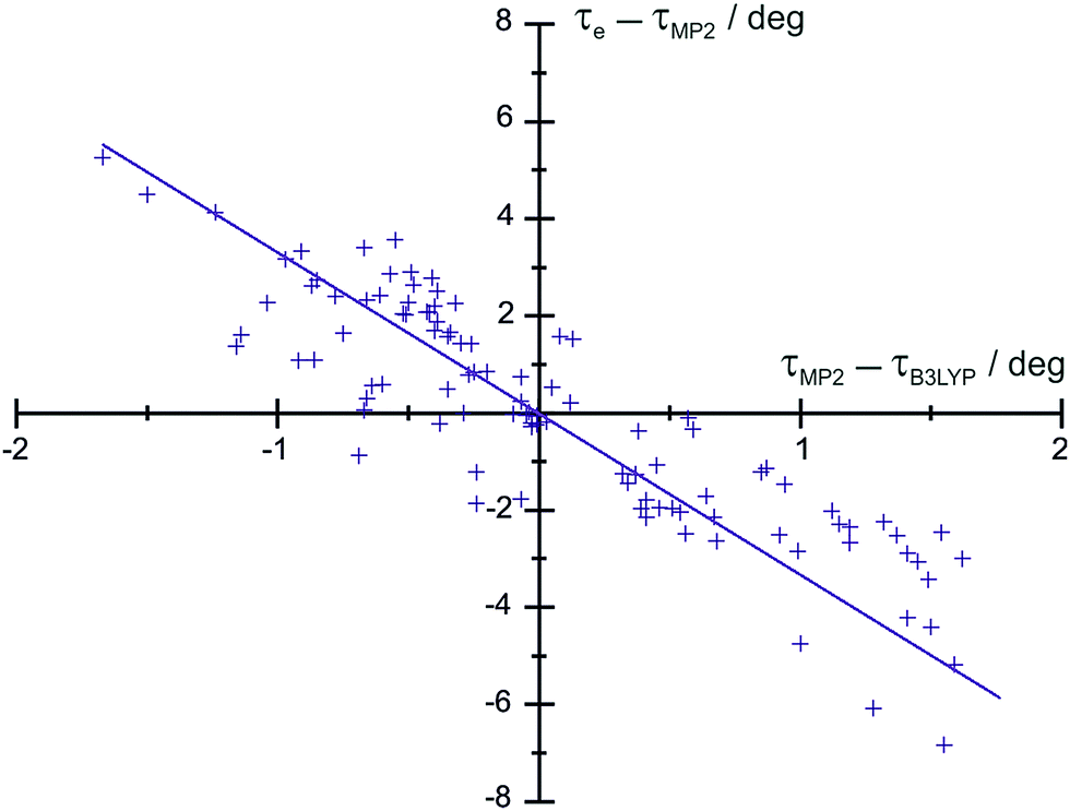Fig. 2 Plot of τ_e–τ[MP2_FC/cc-pVTZ] as a function of τ[MP2_FC/cc-pVTZ]–τ[B3LYP/6-311+G(3df,2pd)] for a selection of molecules in Table S15 (ESI†).

As a further check the predicates for both conformers of fluorocyclohexane and cyclohexanone are compared in Table S16 (ESI†). Obviously, the angles involving the electronegative oxygen atom are less well reproduced but this might perhaps be improved by using the 6-311+G(3df,2pd) basis set instead of cc-pVTZ in the MP2 calculations.

b. Predicates for the CF bond length. The determination of the experimental structure of a fluorine derivative is a difficult problem because there is only one stable isotope for fluorine, making studies of isotopic species impossible. The calculation of a reliable ab initio structure is further complicated by the fact that fluorine is a highly electronegative atom which requires very large basis sets and highly correlated methods. This problem is now tractable for small molecules but, for larger molecules, very few accurate structures have been determined so far. In particular, it is established that the Schomaker–Stevenson equation gives poor results.⁵⁰

For 15 molecules with the C(sp³)F single bond, we tried to estimate the CF bond lengths using the MP2 and B3LYP methods. The B3LYP/6-311+G(3df,2pd) level of theory gives rather unsatisfactory results, as seen in Table 5. The MP2_FC/cc-pVTZ level of theory gives a r_e − r_calc offset of −0.0022(21) Å. However, the problem is that this offset is not constant, as shown in Table 5. The main reason is that fluorine is extremely electronegative and, in such a case, diffuse functions are required. However, replacing the cc-pVTZ basis set by the much larger aug-cc-pVTZ does not significantly improve the situation, in particular the offset and its standard deviation are larger (−0.0054(28) Å). Replacing the basis set by Pople's 6-311+G(3df,2pd) gives much better results with an offset of −0.0042(10) Å, but again this offset is not constant. On the other hand, a linear fit of r_e as a function of r[MP2_FC/6-311+G(3df,2pd)] is very satisfactory (correlation coefficient of 0.999999, F-test as large as 24 246 876), the standard deviation of the fit being 0.0011 Å. In conclusion, to predict the C(sp³)F bond length, the following empirical equation was used

r_e[CF] = 0.99827(20) × r[MP2_FC/6-311+G(3df,2pd)] (3)

Table 5 CF bond lengths (in Å) and charges on the C and F atoms

	r e	MP2_FC/cc-pVTZ	MP2_FC/6^a	B3LYP/6^a	q(F)	q(C)	Δq	Ref.
a 6-311+G(3df,2pd) basis set. b N. Vogt, J. Demaison and H. D. Rudolph, Mol. Phys., 2014, 112, 2873–2883. c J. Breidung, J. Cosléou, J. Demaison, K. Sarka and W. Thiel, Mol. Phys., 2004, 102, 1827–1841. d N. C. Craig, D. Feller, P. Groner, H. Y. Hsin, D. C. McKean and D. J. Nemchick, J. Phys. Chem. A, 2007, 111, 2498–2506. e J. Demaison, J. Breidung, W. Thiel and D. Papoušek, Struct. Chem., 1999, 10, 129–133.
CF4	1.3152	1.3194	1.3174	1.3240	−0.641	2.555	3.196
CClF3	1.3208	1.3227	1.3232	1.3277	−0.638	2.031	2.669
CF3CN	1.3240	1.3288	1.3271	1.3334	−0.631	1.991	2.622
CCl2F2	1.3274	1.3278	1.3303	1.3321	−0.634	1.509	2.143
CHF3	1.3312	1.3338	1.3320	1.3384	−0.651	1.870	2.522
CF3CCH	1.3324	1.3369	1.3356	1.3428	−0.639	1.917	2.556
CHClF2	1.3352	1.3384	1.3375	1.3417	−0.647	1.387	2.034
CCl3F	1.3361	1.3342	1.3406	1.3379	−0.630	0.992	1.622
c-C3H4F2	1.3428	1.3453	1.3448	1.3528
CH2F2	1.3523	1.3544	1.3543	1.3604	−0.664	1.158	1.822
CH2ClF	1.3576	1.3598	1.3610	1.3631	−0.651	0.772	1.423
CF3Li	1.3803	1.3842	1.3827	1.3887	−0.683	1.123	1.805
CH3F	1.3827	1.3809	1.3830	1.3883	−0.660	0.640	1.300
C6H11F eq.	1.3945	1.3954	1.3971	1.4063	−0.670	0.569	1.239	This work
C6H11F ax.	1.4013	1.4015	1.4025	1.4134	−0.672	0.583	1.255	This work

---

Once this result was established, we checked whether it would be possible to improve the Schomaker–Stevenson equation replacing the difference of electronegativities by the difference of charges Δq calculated with the AIM theory.³⁸ There is indeed a correlation between r(CF) and Δq with a Spearman rank correlation coefficient of −0.95. However, this correlation is not quantitative, indicating that other factors apart from the difference of charge are not negligible, as explained in ref. 50.

4. Semiexperimental structure

The semiexperimental equilibrium rotational constants for each direction of the principal axis system, B_e, were calculated from the experimental ground state rotational constants, B₀, using the following equation:

B_e = B₀ + ΔB_vib (4)

where ΔB_vib is the rovibrational correction calculated from the cubic force field obtained at the MP2_FC/cc-pVTZ level of theory.⁵¹ The structure was fitted to both the equilibrium rotational constants of the parent species and all ¹³C species and a full set of predicate values with their estimated uncertainties.

It is possible to estimate the accuracy of the semiexperimental equilibrium rotational constants using the planar moment of inertia P_b = (I_a + I_c – I_b)/2, which should be constant for the parent species and the isotopologues ¹³C1 and ¹³C4. For the equatorial form, its range is 0.00075 u Ų whereas for the axial form it is 0.00242 u Ų. In other words, the rotational constants of the axial form are about three times less accurate than those of the equatorial form, probably because non-rigidity effects are larger for this isomer.

For the equatorial form, the following uncertainties were used for the weighting of the rotational constants (in kHz): 10 for A, and 5 for B and C. For the axial form, the uncertainties are: 100 for A and 50 for B and C. For the predicates, the used uncertainties were 0.002 Å for the CH bond lengths, 0.003 Å for the other lengths, 0.2° for the bond angles and 0.5° for the dihedral angles. The compatibility of these weights was checked using statistical diagnostics as explained in ref. 9.

The rovibrational corrections, the semiexperimental equilibrium rotational constants, residuals of the fit and leverage values h_ii are given in Tables S17 and S18 (ESI†) for the equatorial and axial conformers, respectively.

For the equatorial conformer, the determined parameters in Table 3 are precise, and an examination of the residuals of the fit in Table S17 (ESI†), confirms that the rotational constants and the predicates are compatible. More importantly, inspection of the leverage values, h, shows that: (1) the rotational constants contribute significantly to the determination of the parameters, their median value being 0.71 and being larger than 0.88 for most A rotational constants (a leverage point, defined as h_ii = ∂ŷ_i/∂y_i, where ŷ_i and y_i are the fitted and measured observations, respectively, is high when a small change in the input value causes a large change in the solution, with 0 ≤ h_ii ≤ 1).

For the axial conformer in Table 4 and Table S18 (ESI†), the situation is less favorable, the determined parameters are slightly less precise and the residuals of the fit are one order of magnitude larger. The ground state rotational constants of the ¹³C isotopologues have been determined from very few lines. Thus, it is not possible to exclude that some rotational constants are less accurate. It is also possible that the calculated rovibrational corrections are less accurate.

The semiexperimental equilibrium Cartesian coordinates are given for both conformers in Tables S19 and S20 (ESI†).

Discussion

Accurate equilibrium structures have been determined for the chair forms of equatorial and axial cyclohexane, providing reference data for the molecule and revealing the subtle structural changes between both isomers and the consequences of the fluorine substitution in the cyclohexane ring. The bond parameters, regarded as accurate to 0.001 Å and 0.2°, are given in Tables 3 and 4. The structural determination relies in a mixed estimation fit to predicate (ab initio) bond parameters and equilibrium moments of inertia, each data set accompanied by appropriate uncertainties. The mixed estimation method thus provides a route to equilibrium structure determination at a reduced computational cost.

The most noticeable result is the large values of the CF bond lengths for both conformers in Table 5, the axial value being still longer by almost 0.007 Å. The changes in the heavy atom structural parameters of cyclohexane with the substitution of the fluorine are significant for the C_αC_β distances compared to their distance of 1.5258(6) Å in cyclohexane,⁵² where there is a clear reduction of 0.014 Å for the equatorial form and 0.010 Å for the axial form. The other CC bond lengths and the CH bond lengths are only slightly affected. The dihedral angle τ(CCCC) does not vary much (55.73° in cyclohexane vs. 55.97° and 54.66° for the equatorial and axial forms). Likewise, the bond angle ∠(C1C2C3) is nearly constant (111.11° in cyclohexane and 110.17° and 111.61° for the equatorial and axial forms, respectively). The most affected bond angle should be ∠(C6C1C2), but its value (112.0° in the equatorial form and 112.6° in the axial form) remains close to the cyclohexane value. Thus, the heavy atom ring parameters of cyclohexane appear to be only slightly affected by monosubstitution of the single fluorine atom. In cyclohexanone, the C_αC_β bond length is shortened by 0.014 Å as in equatorial fluorocyclohexane and the C_βC_γ is lengthened by 0.007 Å and, contrary to fluorocyclohexanes, the angle ∠(C6C1C2) is significantly increased, up to 115°.

It is informative to compare the semiexperimental equilibrium structure, r^SE_e, with the empirical substitution structure, r_s. The substitution method⁵³ is widely used to determine molecular structures because it is believed to provide near-equilibrium values. A further advantage is that it is quite simple, the atomic coordinates being obtained from isotopic differences of moments of inertia by using equations formulated by Kraitchman.⁵⁴ However, the key model assumption, i.e., constant rovibrational contributions upon isotopic substitution, is only approximate. Costain has proposed an empirical formula to estimate the coordinates uncertainties,⁵⁵

δ_z = 0.0015/|z| (5)

z being the Cartesian coordinate (in Å). The trouble is that the residual rovibrational contribution increases with the mass of the molecule and as a result Costain's rule becomes much too optimistic.⁵⁶ Another weakness of the method is the presence of small coordinates, i.e. small differences between the moments of inertia. In such as case, frequent for large molecules, the Kraitchman's equations become ill-conditioned and the derived coordinates may be unreliable, or, commonly, produce imaginary coordinates.

We first used Kraitchman's equations with the semiexperimental equilibrium rotational constants of the equatorial conformer (Table S17, ESI†), and found results in nice agreement with the r^SE_e structure, indicating that the rotational constants are accurate (or, more likely, that they have identical systematic errors). Then, we used the ground state rotational constants in Table 1 to determine the r_s structure of the equatorial conformer. The results in Table S21 (ESI†) made evident that the r_s coordinates are at least one order of magnitude less precise than the r^SE_e ones. Furthermore, the small r_s coordinates are not as reliable as anticipated. Still, the most worrying aspect is that the r_s method is not able to correctly predict the small changes in the bond lengths, the r_s values being (in Å): C1C2 = 1.522(4); C2C3 = 1.514(7); C3C4 = 1.532(3) whereas the corresponding r^SE_e values are 1.5122(4); 1.5312(7) and 1.5255(3). In conclusion, for a molecule as fluorocyclohexane, the r_s method does not provide a reliable structure, as already pointed out by Bialkowska-Jaworska et al.²⁰ Unfortunately, this behavior seems to be rather general,^11,12,57 evidencing that the accuracy of the substitution method is limited.

Conclusion

In conclusion, we have demonstrated that the mixed estimation method is operationally superior in terms of accuracy and computational cost to pure ab initio calculations or conventional semiexperimental methods for the determination of accurate equilibrium structures, exploiting the synergy between spectroscopic data and quantum chemical predictions. The application of the mixed estimation method to new chemical systems will expand our description of the factors controlling the molecular structure.

Conflicts of interest

There are no conflicts to declare.

Acknowledgements

Funding from MINECO-FEDER (CTQ2015-68148-C2-2-P) is gratefully acknowledged. N. V., J. D. and H. D. R. thank the Dr Barbara Mez-Starck Foundation (Germany) for support.

References

1. P. Pulay, W. Meyer and J. E. Boggs, J. Chem. Phys., 1978, 68, 5077–5085.
2. Equilibrium Molecular Structures: From Spectroscopy to Quantum Chemistry, ed. J. Demaison, J. E. Boggs and A. G. Császár, CRC Press, Boca Raton, 2011.
3. K. L. Bak, J. Gauss, P. Jørgensen, J. Olsen, T. Helgaker and J. F. Stanton, J. Chem. Phys., 2001, 114, 6548–6556.
4. F. Pawłowski, P. Jørgensen, J. Olsen, F. Hegelund, T. Helgaker, J. Gauss, K. L. Bak and J. F. Stanton, J. Chem. Phys., 2002, 116, 6482–6496.
5. M. Mendolicchio, E. Penocchio, D. Licari, N. Tasinato and V. Barone, J. Chem. Theory Comput., 2017, 13, 3060–3075.
6. C. Puzzarini, J. F. Stanton and J. Gauss, Int. Rev. Phys. Chem., 2010, 29, 273–367.
7. N. Vogt, J. Demaison, J. Vogt and H. D. Rudolph, J. Comput. Chem., 2014, 35, 2333–2342.
8. L. S. Bartell, D. J. Romenesko and T. C. Wong, in Chemical Society Specialist Periodical Report No. 20, ed. G. A. Sim and L. E. Sutton, The Chemical Society, London, 1975, vol. 3, pp. 72–79.
9. J. Demaison, in Equilibrium Molecular Structures: From Spectroscopy to Quantum Chemistry, ed. J. Demaison, J. E. Boggs and A. G. Császár, CRC Press, Boca Raton, 2011, pp. 29–52.
10. D. A. Belsley, Conditioning Diagnostics, Wiley, New York, 1991, pp. 298–299.
11. J. Demaison, N. C. Craig, E. J. Cocinero, J.-U. Grabow, A. Lesarri and H. D. Rudolph, J. Phys. Chem. A, 2012, 116, 8684–8692.
12. N. Vogt, J. Demaison, E. J. Cocinero, P. Écija, A. Lesarri, H. D. Rudolph and J. Vogt, Phys. Chem. Chem. Phys., 2016, 18, 15555–15563.
13. N. Vogt, J. Demaison, S. V. Krasnoshchekov, N. F. Stepanov and H. D. Rudolph, Mol. Phys., 2017, 115, 942–951.
14. N. Vogt, E. P. Altova, D. N. Ksenafontov and A. N. Rykov, Struct. Chem., 2015, 26, 1481–1488.
15. M. Vallejo-López, P. Écija, N. Vogt, J. Demaison, A. Lesarri, F. J. Basterretxea and E. J. Cocinero, Chem. – Eur. J., 2017 DOI:10.1002/chem.201702232 , in press.
16. P. Andersen, Acta Chem. Scand., 1962, 16, 2337–2340.
17. L. Pierce and R. Nelson, J. Am. Chem. Soc., 1966, 88, 216–219.
18. L. Pierce and J. F. Beecher, J. Am. Chem. Soc., 1966, 88, 5406–5410.
19. L. H. Scharpen, J. Am. Chem. Soc., 1972, 94, 3737–3739.
20. E. Białkowska-Jaworska, M. Jaworski and Z. Kisiel, J. Mol. Struct., 1995, 350, 247–254.
21. J. R. Durig, R. M. Ward, K. G. Nelson and T. K. Gounev, J. Mol. Struct., 2010, 976, 150–160.
22. C. A. Stortz, J. Phys. Org. Chem., 2010, 23, 1173–1186.
23. T. J. Balle and W. H. Flygare, Rev. Sci. Instrum., 1981, 52, 33–45.
24. (a) J.-U. Grabow and W. Stahl, Z. Naturforsch., A: Phys. Sci., 1990, 45, 1043–1044; (b) J.-U. Grabow, W. Stahl and H. Dreizler, Rev. Sci. Instrum., 1996, 67, 4072–4084.
25. G. D. Purvis, III and R. J. Bartlett, J. Chem. Phys., 1982, 76, 1910–1918.
26. K. Raghavachari, G. W. Trucks, J. A. Pople and M. Head-Gordon, Chem. Phys. Lett., 1989, 157, 479–483.
27. K. A. Peterson and T. H. Dunning, Jr., J. Chem. Phys., 2002, 117, 10548–10560.
28. C. Møller and M. S. Plesset, Phys. Rev., 1934, 46, 618–622.
29. T. H. Dunning, Jr., J. Chem. Phys., 1989, 90, 1007–1023.
30. M. J. Frisch, J. A. Pople and J. S. Binkley, J. Chem. Phys., 1984, 80, 3265–3269.
31. W. Kohn and L. J. Sham, Phys. Rev. A, 1965, 140, 1133–1138.
32. A. D. Becke, J. Chem. Phys., 1993, 98, 5648–5652.
33. C. Lee, W. Yang and R. G. Parr, Phys. Rev. B: Condens. Matter Mater. Phys., 1988, 37, 785–789.
34. A. G. Császár, Wiley Interdiscip. Rev.: Comput. Mol. Sci., 2012, 2, 273–289.
35. W. D. Allen and A. G. Császár, J. Chem. Phys., 1993, 98, 2983–3015.
36. M. J. Frisch, G. W. Trucks, H. B. Schlegel, G. E. Scuseria, M. A. Robb, J. R. Cheeseman, G. Scalmani, V. Barone, G. A. Petersson, H. Nakatsuji, X. Li, M. Caricato, A. Marenich, J. Bloino, B. G. Janesko, R. Gomperts, B. Mennucci, H. P. Hratchian, J. V. Ortiz, A. F. Izmaylov, J. L. Sonnenberg, D. Williams-Young, F. Ding, F. Lipparini, F. Egidi, J. Goings, B. Peng, A. Petrone, T. Henderson, D. Ranasinghe, V. G. Zakrzewski, J. Gao, N. Rega, G. Zheng, W. Liang, M. Hada, M. Ehara, K. Toyota, R. Fukuda, J. Hasegawa, M. Ishida, T. Nakajima, Y. Honda, O. Kitao, H. Nakai, T. Vreven, K. Throssell, J. A. Montgomery, Jr., J. E. Peralta, F. Ogliaro, M. Bearpark, J. J. Heyd, E. Brothers, K. N. Kudin, V. N. Staroverov, T. Keith, R. Kobayashi, J. Normand, K. Raghavachari, A. Rendell, J. C. Burant, S. S. Iyengar, J. Tomasi, M. Cossi, J. M. Millam, M. Klene, C. Adamo, R. Cammi, J. W. Ochterski, R. L. Martin, K. Morokuma, O. Farkas, J. B. Foresman and D. J. Fox, Gaussian 09, Revision A.02, Gaussian, Inc., Wallingford CT, 2009.
37. (a) H.-J. Werner, P. J. Knowles, G. Knizia, F. R. Manby and M. Schütz, Wiley Interdiscip. Rev.: Comput. Mol. Sci., 2012, 2, 242–253; (b) H.-J. Werner, P. J. Knowles, R. Lindh, F. R. Manby, M. Schütz, P. Celani, T. Korona, A. Mitrushenkov, G. Rauhut, T. B. Adler, R. D. Amos, A. Bernhardsson, A. Berning, D. L. Cooper, M. J. O. Deegan, A. J. Dobbyn, F. Eckert, E. Goll, C. Hampel, G. Hetzer, T. Hrenar, G. Knizia, C. Köppl, Y. Liu, A. W. Lloyd, R. A. Mata, A. J. May, S. J. McNicholas, W. Meyer, M. E. Mura, A. Nicklass, P. Palmieri, K. Pflüger, R. Pitzer, M. Reiher, U. Schumann, H. Stoll, A. J. Stone, R. Tarroni, T. Thorsteinsson, M. Wang and A. Wolf, MOLPRO, 2009.
38. R. F. W. Bader, Atoms In Molecules, Oxford University Press, New York, 1990.
39. (a) J. Cioslowski, A. Nanayakkara and M. Challacombe, Chem. Phys. Lett., 1993, 203, 137–142; (b) J. Cioslowski and P. R. Surján, THEOCHEM, 1992, 255, 9–33; (c) J. Cioslowski and B. B. Stefanov, Mol. Phys., 1995, 84, 707–716; (d) B. B. Stefanov and J. Cioslowski, J. Comput. Chem., 1995, 16, 1394–1404; (e) J. Cioslowski and S. T. Mixon, J. Am. Chem. Soc., 1991, 113, 4142–4145; (f) J. Cioslowski, Chem. Phys. Lett., 1992, 194, 73–78; (g) J. Cioslowski and A. Nanayakkara, Chem. Phys. Lett., 1994, 219, 151–154.
40. J. K. G. Watson, in Vibrational Spectra and Structure, ed. J. R. Durig, Elsevier, Amsterdam, 1977, 6, pp. 1–89.
41. H. M. Jaeger, H. F. Schaefer, III, J. Demaison, A. G. Császár and W. D. Allen, J. Chem. Theory Comput., 2010, 6, 3066–3078.
42. H. D. Rudolph, J. Demaison and A. G. Császár, J. Phys. Chem. A, 2013, 117, 12969–12982.
43. J. Demaison, H. D. Rudolph and A. G. Császár, Mol. Phys., 2013, 111, 1539–1562.
44. C. Puzzarini and V. Barone, Phys. Chem. Chem. Phys., 2011, 13, 7189–7197.
45. N. Vogt, L. S. Khaikin, O. E. Grikina and A. N. Rykov, J. Mol. Struct., 2013, 1050, 114–121.
46. E. Penocchio, M. Piccardo and V. Barone, J. Chem. Theory Comput., 2015, 11, 4689–4707.
47. M. Piccardo, E. Penocchio, C. Puzzarini, M. Biczysko and V. Barone, J. Phys. Chem. A, 2015, 119, 2058–2082.
48. (a) J. M. L. Martin, J. El-Yazal and J.-P. Franco̧is, Mol. Phys., 1995, 86, 1437–1450; (b) A. D. Boese, W. Klopper and J. M. L. Martin, Int. J. Quantum Chem., 2005, 104, 830–845.
49. I. Hargittai and J. B. Levy, Struct. Chem., 1999, 10, 387–389.
50. E. A. Robinson, S. A. Johnson, T.-H. Tang and R. J. Gillespie, Inorg. Chem., 1997, 36, 3022–3030.
51. V. Barone, J. Chem. Phys., 2005, 122, 014108.
52. J. Demaison, N. C. Craig, P. Groner, P. Écija, E. J. Cocinero, A. Lesarri and H. D. Rudolph, J. Phys. Chem. A, 2015, 119, 1486–1493.
53. (a) C. C. Costain, J. Chem. Phys., 1958, 29, 864–874; (b) B. P. Van Eijck, in Accurate Molecular Structures, ed. A. Domenicano and I. Hargittai, Oxford University Press, Oxford, 1992, pp. 47–64.
54. J. Kraitchman, Am. J. Phys., 1953, 21, 17–24.
55. C. C. Costain, Trans. Am. Crystallogr. Assoc., 1966, 2, 157–164.
56. J. Demaison and H. D. Rudolph, J. Mol. Spectrosc., 2002, 215, 78–84.
57. N. C. Craig, J. Demaison, P. Groner, H. D. Rudolph and N. Vogt, J. Phys. Chem. A, 2015, 119, 195–204.

---

Footnote

† Electronic supplementary information (ESI) available: Tables S1–S21. See DOI: 10.1039/c7cp06135h

---