Cancer classification with a network of chemical oscillators

Abstract

We discuss chemical information processing considering dataset classifiers formed with a network of interacting droplets. Our arguments are based on computer simulations of droplets in which a photosensitive variant of the Belousov–Zhabotinsky (BZ) reaction proceeds. By applying optical control we can adjust the time evolution of individual droplets and prepare the network to perform a specific computational task. We demonstrate that chemical classifiers made of droplets can be designed in computer simulations based on evolutionary algorithms. The mutual information between the dataset and the observed time evolution of droplets in the network is taken as the fitness function in the optimization process. We show that a classifier of the Wisconsin Breast Cancer Dataset made of a relatively small number of droplets can distinguish between malignant and benign forms of cancer with an accuracy exceeding 97%. The reliability of the optimized chemical classifiers of this dataset as a function of optimization time, number of droplets involved in data processing and the method of extracting the output information is discussed.

---

1 Introduction

Semiconductors have the dominant position in modern information processing applications, however their physical properties impose restrictions on the environments in which they can operate. In specific systems, e.g. biological ones, or under extreme conditions, e.g. high temperatures, alternative computing strategies can lead to more efficient information processing.^1,2 For instance it is difficult to apply conventional computers at a cellular level in living organisms due to problems such as introduction of electronic components inside the cells, their potential influence on biological processes, electrical energy supply etc. Nevertheless nature has developed computing mechanisms that allow for information processing in cells.^3,4

Studies on non-standard computing strategies, structures and substrates, inspired by chemistry, physics or biology, are encompassed within the research field called unconventional computation.^5–9 In contrast to semiconductor devices, based on von Neumann architecture,¹⁰ unconventional computers interpret the natural time evolution of a medium as a series of information processing operations. In a spatially distributed medium the time evolution of all its parts proceeds simultaneously. As a consequence efficient algorithms executed on an unconventional device are highly parallel.

Among many implementations of unconventional computers, those based on reaction-diffusion (RD) media seem especially interesting. In this paper we focus our attention on information processing with a photosensitive, ruthenium-catalyzed variant of the Belousov–Zhabotinsky (BZ) reaction.¹¹ The BZ reaction is a chemical process in which an organic substrate is catalytically oxidized in an acidic environment. Among reagents of the reaction one can distinguish the activator (HBrO₂), whose concentration can grow autocatalytically, and the inhibitors responsible for suppressing production of the activator. Excitation of such a medium, seen as a rapid increase in the concentration of the activator and next of the inhibitor, can occur when the concentration of the activator exceeds a threshold value or the concentration of the inhibitor fails below a certain level. If the medium is spatially distributed then a local excitation can expand in space via diffusion of the activator and propagate in the form of an excitation pulse (a spike). Such behavior seems qualitatively similar to the propagation of excitations in the nerve system. The FitzHugh–Nagumo model of a spiking neuron^12,13 has similar properties as the Oregonator model of the BZ reaction.¹⁴ Such similarity motivated numerous later studies on information processing based on the BZ reaction. Observation of spike propagation in a medium with the BZ reaction is relatively simple experimentally because the different states of the medium, corresponding to the oxidized and the reduced forms of the catalyst, have different colors. Oscillations of the photosensitive BZ-reaction, can be efficiently controlled with illumination because the blue light activates the catalyst and leads to production of Br⁻ ions that inhibit the reaction.¹⁵ An intensively illuminated medium does not oscillate and it also cannot be excited by a pulse propagating from non-illuminated regions.

Many computational applications of a nonlinear medium relate information with the presence of a spike at specific areas of a non-uniform medium. For example binary logic can be implemented if the logic TRUE and FALSE states are related to the presence or absence of a spike in a selected region. Studies on continuous BZ media, with excitable and non-excitable regions defining the basic information processing operations have been intensively explored.^13,16–21 A new trend in chemical information processing started with experiments on BZ medium encapsulated inside lipid vesicles and immersed in an organic phase.^22–27 This concept seems interesting as a close analogy to compartmentalization in biological systems e.g. the nerve system.

The lipid molecules cover the surface of droplets and stabilize them mechanically.²³ When two droplets come in contact, the lipids form a bilayer at the connection surface²⁸ that enables communication.^{23,25–27,29} This is so because molecules of the BZ activator can diffuse through the bilayer and excite the medium behind, triggering a chemical wave in the neighboring droplet. The interacting droplets can be arranged into larger structures that remain stable for a long time. Large networks of droplets with well defined parameters became accessible using microfluidic techniques.^30,31

It has been demonstrated that BZ-droplets are equally useful for information processing applications as the continuous medium.^32–34 Constructions of logic gates composed of sub-excitable droplets^35,36 and oscillatory ones³⁷ have been described. A typical logic gate needs a few dedicated droplets to operate. Most of the papers concerned with chemical information processing focus on logic gates and end with the conclusion that other information processing devices can be assembled using the gates. Although this statement is correct, such a bottom-up approach is not efficient. For more complex information processing tasks the devices composed of logic gates are large and difficult to build.

In this paper we demonstrate that there are large classes of problems for which the top-down approach seems to be more efficient. As an example we discuss instant machines operating as dataset classifiers. Let us consider a dataset D composed of M records (test cases). A single record contains predictor values p and the assigned category (output class) o and can be represented as a list: (p₁,p₂,…,p_k,o), where k is the number of predictors, fixed for all records in the dataset. The ideal dataset classifier is an algorithm that returns the correct class type if the values of predictors corresponding to a dataset record are used as its input values. Moreover, the dataset of a typical classification problem contains a fraction of all possible cases so it can happen that a given set of input values is not included in it. The algorithm is supposed to guess correctly to which class such a case belongs.

The concept of a dataset classifier generalizes many other information processing tasks. For example, each binary logic operation can be regarded as a classification problem for the dataset composed of M = 4 records. Each record contains two binary predictors representing the arguments of the operation and the binary result of the operation that represents the class type. For a logic gate the dataset contains all possible combinations of the input values. A meaningful realization of a classifier that represents the logic gate should accurately predict the class type.

For a general classification problem a simple construction of a classifier seems as important as its reliability. In this paper we present the construction of a classifier for the Wisconsin Breast Cancer Dataset³⁸ from the Proben1 collection.³⁹ This dataset contains M = 699 records (cases) composed of 10 predictors with the cancer type (benign or malignant) as the output class. Predictors are integer numbers in the range between 1 and 10 describing the physical properties of cells. The mutual information⁴⁰ between all predictors and the output class distribution is 0.93 bit. The analysis of the dataset shows that the mutual information between a pair of predictors and the dataset output reaches its maximum at 0.841 bit for predictors (2, 6). Adding the third predictor significantly increases the maximum mutual information. It becomes 0.916 bit for the predictor triple (1, 2, 6). Therefore, these predictors have been used in this paper. The increase of the number of predictors to 4 increases the mutual information by 0.013 bit only. We may expect that adding the fourth predictor into the evolved structure would result in significantly more time consuming optimization and the accuracy of the resulting structure would not be much better than that obtained for 3 predictors. We demonstrate that a high accuracy classification algorithm of such a dataset can be executed by a network containing a relatively small number of BZ droplets (≤25). The described evolutionary algorithm is general and can be applied for finding the conditions at which the network performs the required classification task in the optimal way.

2 A chemical classifier constructed with oscillating droplets

In this section we define the family of classifiers and briefly describe the evolutionary algorithm used for their optimization. The methods have been already used in a number of our recent papers and the technical details can be found there.^41,42 We study the time evolution of a network of droplets in the time interval [0,t_sim] and relate the output information to the number of excitations observed at a selected droplet within this time interval. The value of t_sim is fixed and is not changed by the optimization procedure.

2.1 The idea of a classifier

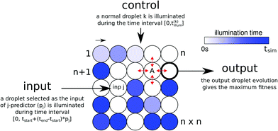
We consider a chemical dataset classifier in the form of a single network of n × n nodes located on a square lattice (Fig. 1). Each node represents a droplet containing oscillating BZ medium. We assume that the oscillations in each droplet can be individually controlled by external illumination with blue light.⁴³ For simplicity we consider just two illumination levels: zero and high. A non-illuminated droplet oscillates whereas a highly illuminated one becomes chemically inactive. Droplets are interconnected with neighbors according to the von-Neumann neighborhood as indicated on droplet A in Fig. 1.

Fig. 1 Illustration of the considered droplet classifier (here shown for n = 5). Circles represent droplets and the intensity of the blue color is proportional to the initial illumination time. The conversion in time to blue color is shown on the horizontal bar. White droplets oscillate from the beginning of the experiment whereas for intensively blue ones the illumination time is close to t_sim. An input is provided by stimulating selected input droplets by illumination. The number of excitations observed at one particular droplet (marked with a wide, black border), in the interval [0,t_sim] is taken as the output. The control “program”, which we obtain by evolution, includes a temporal illumination pattern applied to normal droplets, parameters t_start and t_end and the positions of the input droplets. The numbers to the left and right of the network show that the droplets are labeled row by row starting from droplet 1 in the upper left corner.

The droplets in the classifier are of two types: input and normal (see Fig. 1). They are distinguished according to their functionality in the network. Input droplets are used to feed the values of the predictors of each test case from the dataset into the network. Their illumination times depend on the processed case. The normal droplets transmit and integrate excitations. The illumination time of each normal droplet does not change with the test case. The droplet type along with the illumination pattern for the normal droplets and a few other parameters (described later) can be considered as a program that implements classification functionality into a BZ droplet-based computer.

The values of the predictors are introduced via the illumination times of input droplets in the following way. If a dataset contains k predictors, then k different input types are distinguished. For the dataset considered here k = 3 as we use only the values of predictors p₁, p₂ and p₆ from the dataset. Assume that v^j_s = p^j_s/10 ∈ [0,1] is the normalized value of the predictor s (s = 1,…,k) for a test case j. If a droplet is of the input type, corresponding to the predictor s, then during the simulation of this test case it is illuminated within the time interval [0,t_start + v^j_s(t_end − t_start)]. The values of t_start and t_end (0 ≤ t_start ≤ t_end ≤ t_sim) are the same for all input droplets in a particular network. Yet, they differ from network to network and are optimized by an evolutionary algorithm.

The normal droplets are illuminated over the time interval [0,t⁽ⁱ⁾_illum]. In this interval, a droplet cannot self-excite or be triggered by its neighbors. For a particular network the values of t⁽ⁱ⁾_illum remain the same for all test cases. When the illumination time for a droplet is as long as t_sim, the droplet remains inactive during the whole simulation and can be regarded as an empty slot in the network. The set of values t⁽ⁱ⁾_illum is included in the network program and is a subject of optimization.

The droplet type (normal, input) also undergoes optimization and thus the number and positions of the inputs might vary according to generation. We do not exclude cases where there are multiple droplets of one input type and no input droplet of another.

The output information is extracted from the observation of time evolution of a selected droplet within the time interval [0,t_sim]. The number of excitations of this droplet (the output droplet) should give the maximal mutual information with the output class distribution of the dataset. Let [scr P, script letter P]_o be the set of output classes of the considered dataset [scr P, script letter P]_o = {o_j,j = 1,M}. For each droplet i we introduce the number of excitations sⁱ_j observed for the case j and the sets: [scr S, script letter S]_i = {sⁱ_j,j = 1,M} and [scr S, script letter S]_i[scr P, script letter P]_o = {(sⁱ_j,o_j),j = 1,M} that join the output class with the network's answer. Then the mutual information with the output class distribution [scr P, script letter P]_o is equal to:⁴⁰

I([scr S, script letter S]_i:[scr P, script letter P]_o) = H([scr S, script letter S]_i) + H([scr P, script letter P]_o) − H([scr S, script letter S]_i[scr P, script letter P]_o), (1)

where H denotes the Shannon entropy. Such mutual information can be interpreted as the reduction of uncertainty about the output class when seeing a particular number of excitations, so it reflects the requirements for the best classifier.

If the number of excitations in a droplet is always the same, independent of predictor values then H([scr S, script letter S]_i) = 0 and H([scr S, script letter S]_i[scr P, script letter P]_o) = H([scr P, script letter P]_o). As a result I([scr S, script letter S]_i:[scr P, script letter P]_o) = 0. On the other hand, if the excitation number is perfectly correlated with the dataset output (for example one excitation for a malignant form of cancer and three excitations for the benign one) then H([scr S, script letter S]_i) = H([scr P, script letter P]_o) and H([scr S, script letter S]_i[scr P, script letter P]_o) = H([scr P, script letter P]_o). Now I([scr S, script letter S]_i:[scr P, script letter P]_o) = H([scr P, script letter P]_o) which means that all output information of the dataset can be extracted from the excitation number.

The sets [scr S, script letter S]_i are different for various droplets in the given network. We assume that the droplet with the highest I([scr S, script letter S]_i:[scr P, script letter P]_o) becomes the output of the classifier. Since the mutual information changes during optimization, the position of the output droplet is not fixed and can also vary from generation to generation. We also do not exclude cases in which an input droplet is used as the output one.

2.2 Optimization of BZ networks

An evolutionary algorithm is introduced to optimize the construction of the chemical classifier. We represent a network g as a tuple of the list of functional types for each droplet, the list of the illumination times of the normal droplets , and the two parameters t_start and t_end. The droplet type tp_i = 0 represents the normal droplet. If tp_i = m, where m ∈ {1,…,k}, then the droplet is of the input type corresponding to predictor m. Even for small n, the number of possible networks is enormous and finding an optimal configuration using standard optimization techniques is difficult. In our evolutionary optimization algorithm the initial population of networks (individuals) is generated with random functional types, illumination times of normal droplets and the parameters t_start and t_end (t_start ≤ t_end). Then, the fitness of each network is calculated as I([scr S, script letter S]_i:[scr P, script letter P]_o) for the output droplet. The individuals with the highest fitness are copied into the parental population whereas the others are discarded.

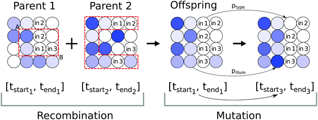
After selecting a sub-population of the most fit individuals a number of randomly selected parents replicate, i.e. their networks are combined to create an offspring individual as illustrated in Fig. 2. A rectangular sub-grid of droplets from Parent 1 constrained by two, randomly selected points A and B replaces the corresponding sub-grid in Parent 2 as illustrated in Fig. 2 to yield a new individual. The illumination interval of input droplets co-evolved with the network is copied from Parent 1 to the Offspring. The newly generated individual is subjected to three, subsequent mutation operators with fixed mutation rates (see Fig. 2) to avoid quick convergence towards the closest local maximum. The mutations are executed in the following order:

Fig. 2 The offspring generation method illustrated for 4 × 4 networks. Randomly selected points A and B in the structure of Parent 1 mark a rectangle, which replaces the corresponding part in Parent 2 to yield a new Offspring during the recombination process. The illumination interval for inputs is copied to the Offspring from Parent 1. Then, during the mutation, droplet types and initial illumination times are modified.

1. Mutation of input illumination interval parameters

Times determining the illumination interval of the droplet with input types, i.e. t^(Offspring)_start and t^(Offspring)_end are selected from the normal distributions with the averages t^(Parent1)_start and t^(Parent1)_end respectively and σ² = 10 as follows:

where [scr N, script letter N](t,σ²) is a random number selected from the normal distribution with average t and variance σ². If t^(Offspring)_start > t^(Offspring)_end both times are swapped i.e. t^(Offspring)_end is replaced with t^(Offspring)_start and vice versa.

2. Mutation of droplet type

We assume that input droplets can change into normal droplets and vice versa. The probability of droplet transformation is p_type = 0.04. Regardless of droplet type the probability of obtaining an input droplet is p_inp = 0.12 and for the normal one 1 − p_inp.

3. Mutation of normal droplet illumination

If a droplet i is of the normal type, then with a probability p_illum = 0.04 its illumination time is mutated. A new illumination time for the Offspring t⁽ⁱ⁾_illum is generated from the normal distribution with the average t⁽ⁱ⁾_illum and σ² = 25.

The values of all probabilities were selected arbitrarily as being reasonably small, but still large enough to produce noticeable changes in network functionality after mutation. They should have little influence on the final, optimized classifier, but definitely decide the rate of convergence towards the optimal solution.

Repeating the recombination and mutation operations yields an offspring population and the evaluation process starts again. In simulations we mixed two evolutionary strategies.^44,45 At the beginning we assumed that only newly generated offspring are transferred to the next generation. This process is similar to natural procreation in the sense that the parents give birth to the offspring population and die afterwards. After 50 generations we preserved the five best parents in the next generation along with the offspring. In this case, an individual with a high fitness value can survive for many generations. The whole evolution scheme is repeated until the specified number of generations is reached.

2.3 The simplified event based model of the BZ-droplet network

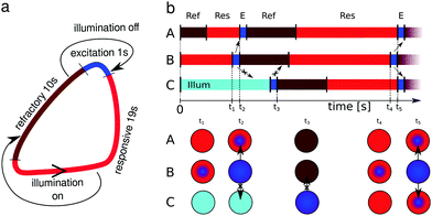
Direct simulations of networks of oscillating droplets based on reaction-diffusion equations are time consuming. Therefore we used a stochastic, time-continuous model⁴⁶ illustrated in Fig. 3. The continuous time makes the simulator more realistic than a cellular automaton, because it requires no roundups to describe the illumination times of normal droplets and the illumination of input droplets related to a given set of predictors. Moreover using a continuous time we can easily introduce randomness to the time a droplet spends in the refractory, responsive and excitation states.

Fig. 3 A simplified model of the time evolution of oscillatory BZ droplets. Colors code phases of the oscillation cycle. (a) The time evolution of a BZ droplet and the influence of illumination on it. The times of each phase refer to the model used. (b) Interactions between neighboring droplets. If the droplet (B) is excited then, after Δt = 1 s, the excitation passes to all neighboring droplets in the responsive phase. No droplet that is illuminated or in the refractory state can be excited.

We divide the oscillation cycle into three phases. A refractory phase begins just after excitation and it is characterized by a high level of inhibitor. In this state a droplet becomes insensitive to chemical excitations coming from its neighbors. Next, the inhibitor concentration decreases with time and after crossing some threshold value the droplet enters the responsive phase in which a stimulus coming from any of the neighbors can lead to an excitation. If no external triggering occurs then the amount of inhibitor drops to a level when self-excitation occurs. The rapid production of activator yields oxidation of the catalyst, seen as the change of droplet color from red to blue and named below as an excitation phase. Bearing in mind the experimental results on interactions between droplets^43,47 we assumed that the durations of the excitation, refractory and responsive phases are 1 s, 10 s, and 19 s respectively. These numbers sum up to the typical oscillation period of 30 s.⁴³ When illumination is applied the droplet is switched into the refractory phase and remains in it. After illumination is turned off, the excitation phase is restored immediately.⁴³

Excitation transfer between two interconnected droplets occurs only if an excitation pulse from one droplet has reached the connection area and the other droplet is in the responsive state cf.Fig. 3b. For millimeter size droplets the self-excitation does not appear in the whole volume of a droplet but starts in its center and propagates outwards.³⁰ Here, to account for this effect, yet make simulations simple, we assumed that an excitation spreads from the center of a droplet regardless of whether it self-excited or was triggered by another droplet. We introduced a propagation time of an excitation pulse t_prop = 1 s, as the time required to travel the distance from the excitation origin to the contact area with the neighboring droplets. Note that t_prop is equal to the duration of the excitation phase hence one can consider a droplet as being in the excited phase if an excitation pulse is visible in any part of it. Even after the excitation phase ends the concentration of the activator remains at a high level for a certain time. Thus we assume that a droplet can activate its neighbors, up to 1 s after its refractory phase started.

A highly nonlinear chemical medium, like the BZ reaction, is very sensitive to internal and external fluctuations. In our event-based model stochastic effects are introduced in the form of normal distributed noise with the standard deviation of 0.05 added to t_prop and to the times when a droplet remains in a particular phase.

3 Results of classifier optimization

The Wisconsin Breast Cancer Dataset contains 699 records (cases) representing cells of two cancer types: with 458 (65.5%) benign and 241 (34.5%) malignant cases. As the starting point, let us consider a classifier in which the output droplet is illuminated during the interval [0,t_obs], so it never gets excited. Let us also assume that the output of the classifier is interpreted as follows: if the number of its oscillations is smaller than 2 then the cancer type is benign. Otherwise it is malignant. Such a classifier has 65.5% accuracy for correct prediction of a randomly chosen record from the dataset because it always states that the form of cancer is not dangerous and such records are in a majority. Having such a level of accuracy in mind we demonstrate that much better classifiers can be obtained as the result of network optimization.

In this section we present the results of simulations. Each result is based on 25 independent simulations of the evolutionary optimization. In each optimization the size of the population was 30 networks. The optimization algorithm contains such arbitrarily selected parameters as: the time within which the evolution is optimized (t_sim) and the time over which the evolution is observed (t_obs). In most of the simulations t_sim = t_obs = 100 s.

Presenting the results we focus on the following topics. First we demonstrate that even a small network of BZ droplets can reliably work as the classifier of the Wisconsin Breast Cancer Dataset.³⁸ Secondly we discuss the influence of various parameters on the classifier quality. Bearing in mind that the optimized structure of a classifier is reached by evolutionary optimization we study how the classifier reliability increases with the number of optimization steps. Next, we check if the classifier quality can be improved at specific relationships between the oscillation period and simulation parameters. The objective time scale of the network is defined by the oscillation period of the BZ reaction. Usually we observe the system for the time for which the structure is optimized, however in general t_sim can be different from t_obs. In the following we demonstrate that the optimized classifiers process information in a highly parallel way and almost all droplets are involved in information processing. We also discuss how the classifier accuracy depends on the number of droplets in the network. Finally we address the problem of classification for a case that is not included in the dataset. To do so, we randomly select 100 cases and exclude them from the dataset used for optimization. After a classifier was optimized on the training data set we tested its reliability on the excluded cases.

3.1 Does the classifier work?

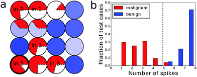
An example of the optimized classifier based on a 4 × 4 network is illustrated in Fig. 4a. The classifier was optimized for 500 generations. Input droplets corresponding to different predictors are marked. The output droplet is indicated by a thick border. The intensity of the blue color for normal droplets increases with illumination time. For example, for the droplet to the right of the input of predictor no. 1 t_ilum = 0 s and for the droplet above the output t_ilum ∼ 100 s. The amount of mutual information contained in each droplet is marked in red in the form of a pie chart where the sector size is normalized to the maximal value of mutual information that can be obtained from the employed inputs.

Fig. 4 (a) The structure, illumination pattern and mutual information content in a 4 × 4 network evolved over 500 generations. The fitness value of the illustrated network equals 0.809 bit. (b) The distribution of the total number of excitations appearing at the output droplet of the 4 × 4 classifier shown in (a) as a function of the cancer type. For each output class the height of the bars is normalized to the number of all cases from this class. The dashed line marks the threshold value used to give a classification rule that yields an accuracy of 97.14%.

The histogram relating the total number of oscillations at an output droplet with the cancer class is shown in Fig. 4b. If we introduce a cut-off at the level of 5 spikes and relate all cases that produce 4 or less oscillations to the malignant form of cancer and all cases leading to 5 or more oscillations to the benign one, then 679 cases of the dataset are classified correctly. This means that that the classification accuracy is 97.14%! It can be even higher if we exclude cases that give exactly 5 oscillations and mark them as doubtful and needing additional consideration. If so then 100% of malignant and 94.6% of benign cases are correctly classified.

3.2 Classifier reliability as a function of optimization time

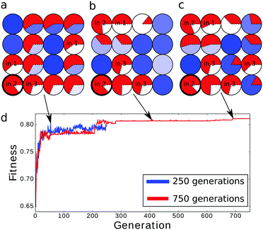
To analyze the influence of the number of optimization steps on the quality of the classifier we compared 4 × 4 networks optimized for 250, 500 and 750 generations. The evolved structures are shown in Fig. 5a–c and the fitness of the best classifier as a function of the optimization step is illustrated in Fig. 5d. As expected the fitness increased with the number of generations in the manner typical for complex optimization problems. The increase was fast at the beginning and then the fitness changed in steps followed by long intervals in which it was almost constant. The fitness value of the most optimized networks is equal to 0.802, 0.809 and 0.811 bit for 250, 500 and 750 optimization steps respectively.

Fig. 5 The structures of the best 4 × 4 network classifiers optimized within (a) 250, (b) 500 and (c) 750 generations. (d) The fitness function obtained in two different simulations: for 250 and 750 generations. The respective fitness values for the networks were 0.802 bit, 0.809 bit and 0.811 bit.

In all optimized classifiers the left bottom droplet (no. 13) is both the output one and works as the input of predictor no. 2. There are significant differences in the locations of inputs and illumination patterns in classifiers obtained within 250 and 500 optimization steps. The fitness functions of classifiers optimized over 500 and 750 generations are only slightly different and the neighborhoods of the output droplet are identical. This suggests that for 4 × 4 networks, optimization requires at least a few hundred generations to approach the final configuration. We have also observed that the number of input droplets increased with the number of optimization steps. Networks optimized for 250, 500 and 750 generations contained 4, 5 and 6 inputs respectively. When comparing the networks optimized for 500 and 750 generations we see that the appearance of an additional input droplet leads to significant differences in the mutual information of droplets located in the right part of the network.

The histograms relating the number of spikes to the cancer type are shown in Fig. 4b, 6a and b. In all cases we can apply the same cut-off at the level of 5 spikes to distinguish the malignant and benign forms of cancer. Surprisingly the accuracy of the classifier optimized for 500 generations was slightly higher (97.14%) than of the one optimized for 750 steps (97.00%). The difference comes from a single malignant case that was correctly classified by the first classifier and incorrectly by the second one. On the other hand the higher mutual information of the classifier optimized for 750 generations is related with the more compact distribution of benign cases: there are no benign cases that produce a single output spike.

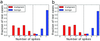Fig. 6 Histograms relating the numbers of output excitations with the cancer type for the networks shown in (a) Fig. 5a and (b) Fig. 5c. A single threshold rule yields accuracies of: (a) 96.57% and (b) 97.00%.

3.3 The influence of t_sim and t_obs on simulation results

At the beginning let us consider the situation in which the excitations of the output droplet are counted for time t_obs that is different from the classifier optimization time t_sim. We start with the classifier illustrated in Fig. 4, optimized for t_sim = 100 s. Using this structure, we performed dataset classification with t_obs set to 50 s or 200 s. The histograms relating the observed numbers of excitations at the output droplet with the cancer type are shown in Fig. 7. The values of mutual information between the number of oscillations at the output droplet and the dataset output were 0.721 bit and 0.813 bit, so it was significantly reduced for t_obs = 50 s. For t_obs = 50 s the droplets with 50 s ≤ t_illum ≤ 100 s did not contribute to the output signal and the behavior of the whole network was changed. The corresponding histogram of excitation numbers is shown in Fig. 7a. Obviously the numbers of excitations are smaller than for t_obs = 100 s (cf.Fig. 4b). Still introducing the cut-off at 2 spikes we obtain quite a high classification accuracy (95.56%) despite the large reduction of fitness with respect to the t_obs = 100 s case. Such a high reliability can be explained by seeing that in the optimized classifier (cf.Fig. 4a) there are droplets with a short t_illum around the output one. They are fully active even for t_obs = 50 s.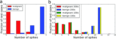

Fig. 7 Output signal from a network evolved with t_sim = 100 s and observed for (a) 50 s and (b) 200 s. Fitness value and classification accuracy for (a) drops to 0.721 bit and 95.56%. In (b) fitness increased slightly to 0.813 bit and accuracy remains at 97.14%. For comparison we plotted the signal from Fig. 4b (hatched bars on the right) with the argument shifted by 3 spikes.

If t_obs = 200 s, then the histogram illustrated in Fig. 7b is almost identical to the one for t_obs = 100 s, but the arguments are increased by 3 spikes. Surprisingly the mutual information between the dataset output and the number of excitations at the output droplet is slightly higher than that for the classifier optimized with t_obs = 100 s. The classification accuracy based on the cut-off at 8 spikes is 97.14% and equals that of the original classifier. This suggests that after 100 s, when all of the droplets were not perturbed by illumination, the network was synchronized by a single pacemaker forcing the same number of excitations in each droplet. Such a phenomenon is frequently observed in experiments with networks of BZ droplets.³⁰

We can conclude by stating that classification is a transient phenomenon. The major part of data processing is done a short time after information is introduced into the network.

It is not surprising that the reliability of a classifier was not increased if the data were collected for times different than the one the classifier was optimized for (t_sim ≠ t_obs). In the analysis below we present results for t_sim = t_obs ≠ 100 s. We studied two cases: t_sim = t_obs = 50 s and t_sim = t_obs = 200 s, keeping the same model of the BZ reaction with a 30 s period. The networks and the histograms relating the number of output excitations with the cancer type are shown in Fig. 8. In all cases the networks were evolved for 500 generations. For t_sim = 50 s the fitness of the best output was 0.783 bit. The cut-off at 3 spikes leads to a classification accuracy of 96.71%. This is higher than in the case discussed above, when the structure optimized for t_sim = 100 s was observed for t_obs = 50 s. For t_sim = 200 s the fitness of the best classifier was 0.825 bit. The corresponding histogram is shown in Fig. 8e and the distribution of spikes is more complex than those in the previous cases. Now it is not obvious how to select the cut-off. Obviously it should be larger than 8 spikes (cf.Fig. 7b). For cut-offs at the levels of 10, 11 and 12 spikes we obtain classification accuracies of 96.71%, 95.99% and 96.14% respectively. All these values are below the reliability of the classifier optimized for t_sim = 100 s despite the higher fitness. This result indicates that there is a relationship between the period of oscillations and t_sim = t_obs that leads to the maximum reliability of a classifier. To confirm this we plan to perform simulations based on longer classifier optimization.

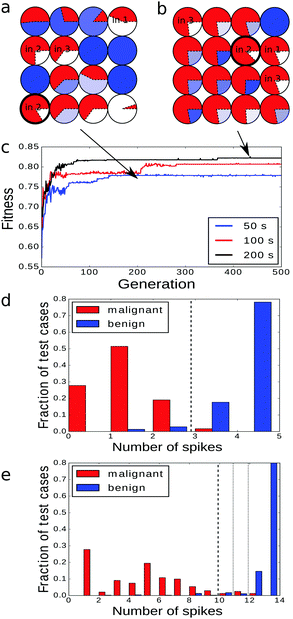Fig. 8 (a) The fitness function as a function of optimization progress for 4 × 4 networks with t_sim set to 50 s, 100 s and 200 s. Structures of the best classifiers for the simulation times 50 s and 200 s are shown in (b) and (c) respectively. (d and e) The histograms illustrating how the number of output droplet excitations are related to the cancer type t_sim = 50 s and 200 s. The results for the classifier optimized with t_sim =100 s are presented in Fig. 4.

3.4 The parallelism of information processing

Efficient unconventional algorithms are parallel and executed by the computing medium as a whole. In order to verify if all droplets of the network contribute to the classification we performed a series of simulations with the network shown in Fig. 4a in which one selected, normal droplet was illuminated within the time interval [0,t_sim], and so deactivated during t_obs. The fitness values of the reduced networks with the corresponding classification accuracy are presented in Table 1. In all cases the droplet with the highest fitness is considered as the output one. These results indicate that almost every droplet has a role in sustaining the high mutual information content and accuracy of the classifier. Only the deactivation of droplets 12 or 16 located far from inputs and the output did not affect the functionality of the network. Thus one can expect that information processing inside the network occurs in a highly parallel manner.

Table 1 Fitness and classification accuracy for the 4 × 4 network shown in Fig. 4a if a selected normal droplet was illuminated for the whole simulation time (t⁽ⁱ⁾_illum = t_sim = 100 s). The illumination of droplets indicated with arrows had the largest (14) or negligible (16) influence on classification accuracy

Illuminated droplet no i	Network fitness [bit]	Classification accuracy (%)
3	0.736	94.71
4	0.756	94.85
5	0.780	96.85
6	0.719	94.56
7	0.807	97.00
8	0.780	95.71
9	0.800	96.42
11	0.807	97.00
12	0.809	97.14
→14	0.718	94.42
→16	0.809	97.14

---

To examine in detail to what extent a missing droplet changes the information content in every node of the network we discuss two cases: (i) droplet 16 that has a negligible effect on classification accuracy and (ii) droplet 14 that generates its largest decrease. In scenario (i) the deactivation of droplet 16 does not seem to have any effect on the mutual information in other droplets. The negligible role of droplet 16 in the functioning of the network can be explained firstly by its location in the right bottom corner, far from the output and secondly by the fact that even without external deactivation it was illuminated for a long time t⁽¹⁶⁾_illum ∼ 75 s. In fact, when droplet 16 was deactivated the output signal at droplet 13 (data not shown) was the same as for the original network (see Fig. 4b). In scenario (ii), illustrated in Fig. 9, the right neighbor of the original output droplet 13 was deactivated and blocked contacts between the output and the input of predictor no. 6. Isolation of droplet 13 from the rest of the network resulted in a large decrease in its mutual information content. As anticipated its signal reduced to a simpler form. The number of excitations ranged from 1 to 5 as shown in Fig. 9b. Based on such a signal the classifier accuracy decreased to 92.42%. In the network with deactivated droplet 14 the time evolution of droplet 1 had the largest mutual information. The signal at droplet 1 (see Fig. 9c) remained almost the same as in the original network. The same classification accuracy is obtained if droplet 1 is used as the output of the original network.

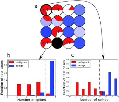Fig. 9 (a) Structure of a 4 × 4 network from Fig. 4a in which droplet 14 was blocked externally during the whole simulation (marked schematically with black color). Note that when droplet 14 is blocked droplet 1 is selected as the output. Histograms representing the output signal in the network from figure (a) at droplet (b) 13 and (c) 1. Classification accuracies for the signals shown are: (b) 92.42% and (c) 94.42%.

3.5 Does the classifier accuracy increase with the number of droplets?

Until now we have concentrated our attention on classifiers based on 4 × 4 networks of droplets. Now we compare their reliability with classifiers based on a single droplet (1 × 1) and on 2 × 2, 3 × 3 and 5 × 5 droplet systems. Obviously, a larger network should have at least as high a reliability as a smaller one because we can map a small classifier into a large one and deactivate the remaining droplets.

If one droplet is considered it should function both as the input and as the output. Without loss of generality we can assume that t_start = 0 and t_end = t_sim (here t_sim = 100 s) and thus no optimization is required. If the droplet was used as an input of predictor 1, 2 or 6 then the calculated mutual information was 0.419 bit, 0.642 bit or 0.571 bit respectively. The corresponding accuracies of these classifiers, with the cut offs set at 1, 2 or 2 spikes, were 82.8%, 89.55% or 90.13%.

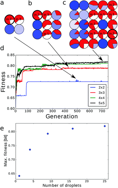
The classifiers based on 2 × 2, 3 × 3 and 5 × 5 droplet networks were optimized for 750 generations. The obtained structures are shown in Fig. 10a–c (and Fig. 5c for the 4 × 4 configuration). In all of them the output droplet is also the input for predictor no. 2 that for a single-droplet classifier produced the highest mutual information. The fitness evolution for all considered network sizes, presented in Fig. 10d, indicates that the increase in fitness value is faster for larger classifiers. On the other hand the time needed to reach a stationary value of fitness also increases with network size. As expected the maximum fitness grows with the network size (see Fig. 10e). The dependence of maximal fitness on the network size suggests that the fitness of n × n droplet networks for n ≥ 6 is saturating. Thus, one can expect that up-scaling the classifier over 25 droplets does not significantly increase classification accuracy.

Fig. 10 The structures of the best (a) 2 × 2, (b) 3 × 3, and (c) 5 × 5 classifiers evolved within 750 generations. (d) Fitness evolution as a function of optimization progress. (e) Maximal fitness values for 2 × 2 (0.736 bit at 495th generation), 3 × 3 (0.793 bit at 426th generation), 4 × 4 (0.811 at 706th generation) and 5 × 5 networks (0.820 at 706th generation) as a function of the number of droplets the classifier is formed with.

The histograms presenting the number of excitations at the output droplet as a function of cancer type are given in Fig. 11 and for the 4 × 4 network in Fig. 6b. The cut-off value increases with the network size. It equals 4 excitations for the 2 × 2 and 3 × 3 networks, 5 for the 4 × 4 network and 6 for 5 × 5 droplet systems. The corresponding accuracies of these classifiers are: 95.14%, 95.85%, 97% and 96.57% respectively. These values are quite similar and thus we are not able to conclude if the classifier based on the 4 × 4 network performs better than the one constructed with the 5 × 5 droplet system. The slightly reduced accuracy of the 5 × 5 network can be related to the largest size of parameter space in which optimization is performed and the limited number of generations in the procedure.

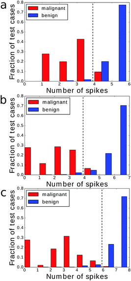Fig. 11 Distributions of excitation numbers at the output of (a) 2 × 2, (b) 3 × 3, and (c) 5 × 5 networks from Fig. 10a–c. Classification accuracy based on a single threshold is equal to: (a) 95.14%, (b) 95.85% and (c) 96.57%.

3.6 The predictive power of network classifiers

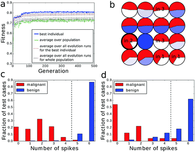
It is expected that a good classifier recognizes correctly the cases used during its teaching process and, based on the gathered knowledge, can make a correct recognition of the cases not included in the dataset. To verify if the considered chemical classifiers have such an ability we divided the dataset into two subsets: the training dataset with 599 cases and the test dataset containing the remaining 100 cases. The test dataset contained 50 malignant cases and 50 benign cases, which were randomly selected. Within the optimization process only the training dataset was used. Afterwards, the optimized network was evaluated with the cases from the test dataset only. For the selected training dataset the one-droplet-based classifier had an accuracy of 84.63%, 92.00% or 92.65% depending on whether the droplet was used as the input of p₁, p₂ or p₆. However, the accuracy of the prediction for cases in the test dataset drops to 72%, 66% and 58% respectively. Therefore, the predictive power of a one-droplet-based classifier is not much better than a random binary answer. The results are more encouraging if networks of droplets are employed.

The analysis below is limited to 4 × 4 network classifiers evolved within 500 generations since they yielded the highest classification accuracy for the original dataset (cf.Fig. 4). The fitness evolution plot and the structure optimized for the subdivided dataset are shown in Fig. 12a and b. The fitness value of the best network was 0.817 bit, which is higher than the fitness for a network optimized with the original dataset (cf.Fig. 5). Furthermore, for the reduced dataset, classifiers with the fitness value above 0.8 bit were obtained in a smaller number of generations (≤100) while for the full dataset ≥200 generations were required to optimize a network with a similar fitness. Such an improvement is related to a larger fraction of benign cases in the reduced dataset (68.11%) than in the original one (65.5%). For the considered method of information readout (cf.Fig. 4b) the probability of the correct classification of the benign type is higher than that for the malignant one.

Fig. 12 (a) Fitness evolution and (b) structure of a classifier optimized with the training dataset within 500 generations. The output signal of the network fed with the cases from (c) the training and (d) the test dataset. The dashed line indicates a threshold that leads to the classification rule with an accuracy of 98% for the training dataset. The same threshold value applied for the test dataset gives an accuracy of 88%.

The histograms representing the output signal for the cases from the training and the test datasets are presented in Fig. 12c and d respectively. The accuracy obtained for the training dataset was 98%. If the same classification rule was applied to the cases from the test dataset the accuracy was lower and equal to 88%. Yet, one can see that even in this case both peaks for both classes are well separated. Therefore the optimized classifier is able to make a correct guess in a large fraction of cases that were not included in the training dataset.

4 Conclusions

In this paper, considering the Wisconsin Breast Cancer Dataset as an example, we demonstrated that evolutionary algorithms can be successfully used to design chemical classifiers based on interacting BZ droplets. We have shown that even a simple network, composed of a small number of droplets can be optimized to perform the required classification task with an accuracy exceeding 97%. Moreover, we demonstrated that network based classifiers do have predicting power: operating on the cases not included in the training dataset they are able to recognize the cancer type with an accuracy exceeding 88%. In our opinion this result is surprising. Usually it is expected that one should have some knowledge of the problem to make predictions. It is hard to believe that a network composed of a few interacting chemical oscillators can understand what kind of information it processes. Yet, the applied evolutionary algorithm was able to optimize the interactions inside the network such that the essential correlations between the predictor values and the cancer type are built into the droplet network and the classifier gives correct answers for a large fraction of cases.

We think that it would be difficult to obtain a similar result with the bottom-up approach to the classification problem. To illustrate the difficulties let us assume that all values in the dataset records (p₁,p₂,…,p_k,o) are binary (i.e. p_i ∈ {0,1} for i = 1, k and o ∈ {0,1}). For such a dataset the bottom-up construction of a classifier that accurately classifies the dataset cases is straightforward. Let us assign the logic values TRUE and FALSE to numbers 1 and 0 respectively and consider a subset of the dataset S (S ∈ D) such that a record (p₁,p₂,…,p_k,o) ∈ S if o = 1. Thus S is a dataset containing all elements of D of the TRUE type. Let us assume that there are N records in the dataset S (N ≤ M). The classifier of the dataset D can be directly written as the logic function F defined on a set of input values (r₁,r₂,…,r_k) as follows:

where (p_1m,p_2m,…,p_km) ∈ S for m = 1,N. The function F defined as the alternative of conjunctions checks if the input (r₁,r₂,…,r_k) appears in the dataset S and in such a case returns the logic value TRUE. In all other cases its value is FALSE, so it perfectly solves the classification problem.

If the dataset S contains more than half of the dataset records, then an alternative definition of a classifier based on records in the dataset D/S leads to a simpler function:

where (p_1m,p_2m,…,p_km) ∈ D/S for m = 1, M − N. As seen, it checks if the input values are in the dataset D/S and if so returns the value FALSE. In all other cases the logic value of G(r₁,r₂,…,r_k) is TRUE.

The idea of classifiers shown above can be easily generalized for the case when the values of predictors are rational. In such a case we should approximate their values by a finite binary fraction and compare the subsequent bits of expansion with the input. Although, the algorithms based on logic F or G functions perfectly classify the dataset D their predicting power is very limited, because all cases not included in D are mapped onto the same logic value.

The classifiers based on logic F or G functions can be useful if a negligible number of possible cases are not included in D. However, it seems extremely difficult to use them for practical construction of droplet based classifiers because at least a few droplets are needed for a single logic operation.^{32–34,36,37} Thus, even for a small dataset of circa 100 records, the direct bottom-up construction of a classifier requires thousands of interacting droplets located in a precisely defined geometry.

Our work has suggested a number of issues that can be important for future studies on chemical classifiers. The mutual information, combining the network evolution with the output class of a record seems a good candidate for the fitness function in the optimization algorithm. It is easy and fast to calculate and properly reflects the trend. However, it is not perfect. We have observed cases when a network, characterized by a slightly smaller value of the mutual information, had a greater classification accuracy than a network containing higher mutual information. Thus in our opinion, more precise optimization algorithms should be oriented towards increasing the classification accuracy directly.

Within our method of output information coding, classification is a transient phenomenon related to the number of excitations in a specific time interval. However the described classifiers can be modified to code the output information in a stationary state of the system. To do so a chemical counter of excitations⁴⁸ has to be linked with the output droplet by a channel that opens in the time interval [0,t_obs]. Then, the number of excitations is coded in the final, stationary state of the memory.

The major part of data processing is done a short time after information is introduced into the network. The results presented in Section 3.3 suggest that the classifier accuracy has a maximum at a certain ratio between t_sim and the period of medium oscillations. We plan to investigate the effect considering classifiers optimized for a much larger number of generations.

In practical application both reliability and simplicity of construction are important. The method of droplet deactivation, used in the Section 3.4 to prove parallelism in information processing, can be applied to analyze the information flow through the network and trace the droplets that can be omitted without loss of classifier accuracy. Results presented in Section 3.5 indicate that functioning of the classifiers depends on the number of droplets they are composed of. Therefore one has to take into consideration how far a given network can be down-(or up-)scaled before its classification accuracy drops below a required level (or its size exceeds some external constraints).

In the paper we have considered droplets forming a square lattice. We have also performed calculations for droplets located on a two-dimensional hexagonal lattice. In such a system a droplet can have up to 6 neighbors, thus the number of connections increases by 50% compared to the studied network. Optimization of 4 × 4 and 5 × 5 droplet classifiers with the hexagonal geometry leads to mutual information that differs by 0.003 bit if compared with the classifiers described in the text. We can conclude that the geometry of droplet connections does not significantly change the accuracy of the Wisconsin Breast Cancer Dataset classifier.

The presented idea of a chemical classifier can be applied to other networks of interacting chemical oscillators. Considering potential applications it is important to identify factors that can inhibit oscillations in individual droplets. If these factors are directly related with the concentrations of reagents or other physico-chemical properties of the investigated system then a classifier can operate autonomously and does not require an additional interface to acquire input information. If so the chemical classifiers can be made small enough to find applications in such areas as intelligent drug delivery or deep space research.

Conflicts of interest

There are no conflicts to declare.

Acknowledgements

The work was supported by the Polish National Science Centre grant UMO-2014/15/B/ST4/04954.

References

1. J. Gorecki, J. N. Gorecka, B. Nowakowski, H. Ueno and K. Yoshikawa, Phys. Chem. Chem. Phys., 2016, 18, 20518–20527.
2. J. Gorecka and J. Gorecki, Phys. Chem. Chem. Phys., 2005, 7, 2915–2920.
3. D. Bray, Nature, 1995, 376, 307–312.
4. S. Tay, J. J. Hughey, T. K. Lee, T. Lipniacki, S. R. Quake and M. W. Covert, Nature, 2010, 466, 267.
5. T. Gramss, S. Bornholdt, M. Gross, M. Mitchell and T. Pellizzari, Non-Standard Computation: Molecular Computation – Cellular Automata – Evolutionary Algorithms – Quantum Computers, Wiley-VCH Verlag GmbH & Co. KGaA, 2005.
6. C. Calude and G. Paun, Computing with cells and atoms: an introduction to quantum, DNA and membrane computing, CRC Press, 2000.
7. A. Adamatzky, B. D. L. Costello and T. Asai, Reaction-Diffusion Computers, Elsevier Science Ltd, Amsterdam, Netherlands, 2005.
8. A. Adamatzky, L. Bull and B. D. L. Costello, Unconventional computing, Luniver Press, 2007.
9. A. Adamatzky, Advances in Unconventional Computing: Volume 1: Theory, Springer, 2017, vol. 22.
10. J. Von Neumann, John von Neumann: selected letters, American Mathematical Soc., 2005, vol. 27.
11. A. N. Zaikin and A. M. Zhabotinsky, Nature, 1970, 225, 535–537.
12. R. FitzHugh, Biophys. J., 1961, 1, 445–466.
13. I. Motoike and K. Yoshikawa, Phys. Rev. E: Stat. Phys., Plasmas, Fluids, Relat. Interdiscip. Top., 1999, 59, 5354.
14. R. J. Field and R. M. Noyes, J. Chem. Phys., 1974, 60, 1877–1884.
15. L. Kuhnert, Nature, 1986, 319, 393.
16. A. Toth and K. Showalter, J. Chem. Phys., 1995, 103, 2058–2066.
17. O. Steinbock, A. Toth and K. Showalter, Science, 1995, 267, 868.
18. O. Steinbock, P. Kettunen and K. Showalter, J. Phys. Chem., 1996, 100, 18970–18975.
19. J. Sielewiesiuk and J. Gorecki, J. Phys. Chem. A, 2001, 105, 8189–8195.
20. A. Adamatzky and B. D. L. Costello, Phys. Rev. E: Stat., Nonlinear, Soft Matter Phys., 2002, 66, 046112.
21. K. Yoshikawa, I. Motoike, T. Ichino, T. Yamaguchi, Y. Igarashi, J. Gorecki and J. N. Gorecka, Int. J. Unconv. Comput., 2009, 5, 3–37.
22. V. K. Vanag and I. R. Epstein, Phys. Rev. Lett., 2001, 87, 228301.
23. J. Szymanski, J. N. Gorecka, Y. Igarashi, K. Gizynski, J. Gorecki, K.-P. Zauner and M. D. Planque, Int. J. Unconv. Comput., 2011, 7, 185–200.
24. V. K. Vanag and I. R. Epstein, Proc. Natl. Acad. Sci. U. S. A., 2003, 100, 14635–14638.
25. M. Toiya, V. Vanag and I. Epstein, Angew. Chem., Int. Ed., 2008, 47, 7753–7755.
26. M. Toiya, H. O. Gonzalez-Ochoa, V. K. Vanag, S. Fraden and I. R. Epstein, J. Phys. Chem. Lett., 2010, 1, 1241–1246.
27. S. Thutupalli and S. Herminghaus, Eur. Phys. J. E: Soft Matter Biol. Phys., 2013, 36, 1–10.
28. P. H. King, G. Jones, H. Morgan, M. R. de Planque and K.-P. Zauner, Lab Chip, 2014, 14, 722–729.
29. V. K. Vanag and I. R. Epstein, Phys. Rev. E: Stat., Nonlinear, Soft Matter Phys., 2011, 84, 066209.
30. J. Guzowski, K. Gizynski, J. Gorecki and P. Garstecki, Lab Chip, 2016, 16, 764–772.
31. K. Torbensen, F. Rossi, S. Ristori and A. Abou-Hassan, Lab Chip, 2017, 17, 1179–1189.
32. A. Adamatzky, B. De Lacy Costello and L. Bull, Int. J. Bifurcation Chaos Appl. Sci. Eng., 2011, 21, 1977–1986.
33. A. Adamatzky, J. Holley, L. Bull and B. De Lacy Costello, Chaos, Solitons Fractals, 2011, 44, 779–790.
34. J. Holley, A. Adamatzky, L. Bull, B. De Lacy Costello and I. Jahan, Nano Commun. Netw., 2011, 2, 50–61.
35. A. Adamatzky, B. De Lacy Costello, L. Bull and J. Holley, Isr. J. Chem., 2011, 51, 56–66.
36. J. Holley, I. Jahan, B. De Lacy Costello, L. Bull and A. Adamatzky, Phys. Rev. E: Stat., Nonlinear, Soft Matter Phys., 2011, 84, 056110.
37. J. Gorecki, J. N. Gorecka and A. Adamatzky, Phys. Rev. E: Stat., Nonlinear, Soft Matter Phys., 2014, 89, 042910.
38. K. Bache and M. Lichman, UCI Machine Learning Repository, 2013, http://https://archive.ics.uci.edu/ml/datasets/Breast+Cancer+Wisconsin+(Original).
39. L. Prechelt, Proben1: A set of neural network benchmark problems and benchmarking rules, Fakultat fur Informatik, Universitat Karlsruhe, Germany technical report, 1994.
40. T. M. Cover and J. A. Thomas, Elements of information theory, John Wiley & Sons, 2012.
41. K. Gizynski, G. Gruenert, P. Dittrich and J. Gorecki, Evol. Comput., 2017, 25 DOI:10.1162/EVCO_a_00197.
42. K. Gizynski and J. Gorecki, Comput. Meth. Sci. Technol., 2016, 22, 167–177.
43. K. Gizynski and J. Gorecki, Phys. Chem. Chem. Phys., 2017, 19, 6519–6531.
44. H.-P. Schwefel, Numerische Optimierung von Computer-Modellen mittels der Evolutionsstrategie: mit einer vergleichenden Einführung in die Hill-Climbing-und Zufallsstrategie, Birkhäuser, Basel, Switzerland, 1977.
45. H.-P. Schwefel, Numerical Optimization of Computer Models, John Wiley & Sons, Inc., New York, NY, 1981.
46. G. Gruenert, J. Szymanski, J. Holley, G. Escuela, A. Diem, B. Ibrahim, A. Adamatzky, J. Gorecki and P. Dittrich, Int. J. Unconv. Comput., 2013, 9, 237–266.
47. G. Gruenert, K. Gizynski, G. Escuela, B. Ibrahim, J. Gorecki and P. Dittrich, Int. J. Neur. Syst., 2015, 25, 1450032.
48. J. Gorecki, K. Yoshikawa and Y. Igarashi, J. Phys. Chem. A, 2003, 107, 1664–1669.

---