Efficient simulation of ultrafast magnetic resonance experiments

Abstract

Magnetic resonance spectroscopy and imaging experiments in which spatial dynamics (diffusion and flow) closely coexists with chemical and quantum dynamics (spin–spin couplings, exchange, cross-relaxation, etc.) have historically been very hard to simulate – Bloch–Torrey equations do not support complicated spin Hamiltonians, and the Liouville–von Neumann formalism does not support explicit spatial dynamics. In this paper, we formulate and implement a more advanced simulation framework based on the Fokker–Planck equation. The proposed methods can simulate, without significant approximations, any spatio-temporal magnetic resonance experiment, even in situations when spatial motion co-exists intimately with quantum spin dynamics, relaxation and chemical kinetics.

---

1. Introduction

Spatial coordinates are more convenient in magnetic resonance than temporal ones – unlike the indelible past, any voxel in the [Doublestruck R]³ can be accessed repeatedly. The use of spatial coordinates as replacements for temporal ones was the key idea behind the “ultrafast” NMR methods proposed in 2002 by the Frydman group.¹ Those methods enabled the study of chemical² and biological^3,4 processes on a time scale that was not previously accessible to multi-dimensional NMR.⁵ Applied to MRI, the same approach enabled fast localised acquisition of 2D spectra.⁶ Another useful application of the same idea is the family of “pure-shift” NMR experiments,⁷ fine-tuned at Manchester University around 2010⁸ – they finally achieved the dream of eliminating homonuclear J-couplings.

Spatial dimensions do have their problems though – the biggest one is the presence of uncontrolled dynamics (e.g. diffusion and convection) that is coupled to quantum mechanical evolution.^9,10 Pulse sequence design must therefore rely on detailed modelling of simultaneous spatial, chemical and quantum dynamics, which would be wonderful if only the required theory and software existed: the usual Liouville–von Neumann equation is not good enough because there is no easy way to combine diffusion and hydrodynamics¹¹ with quantum mechanical spin evolution. The primary nuisance is the J-coupling^12,13 – it dephases transverse magnetisation and generates undesirable modulations in echo trains.^13,14

Very complicated systems of precisely this kind are emerging in all areas of magnetic resonance: hyperpolarised pyruvate imaging¹⁵ requires simultaneous modelling of quantum spin dynamics, diffusion, hydrodynamics, chemical kinetics and spin relaxation theory; the same applies to hyperpolarised singlet state imaging.¹⁶ Pure-shift NMR,⁸ ultrafast NMR,¹⁷ metabolite-selective imaging,¹⁸ PARASHIFT contrast agents¹⁹ and other similar recent developments are all united by their theory and simulation infrastructure requirements that are a level above anything that is currently available.

The methods currently used in MRI (Bloch–Torrey equations,^20,21 distributed Bloch equations,^22,23k-space Bloch equations,²⁴etc.) are very well developed,²⁵ but insufficient for ultrafast NMR or singlet state MRI because all of those methods are built around Bloch equations for the spin degrees of freedom; this makes accurate treatment of coupled multi-spin systems impossible. Some methods (split propagation,²⁶ random-walk averaging,²⁷etc.) do treat spin dynamics at the density matrix level, but introduce diffusion externally in an approximate way.²⁸

To our knowledge, the only formalism that simultaneously supports diffusion, hydrodynamics, chemical kinetics and Liouville-space spin dynamics in a general and computationally affordable way is the Fokker–Planck equation.^29–31 In this paper, we present the corresponding algebraic and numerical framework, and illustrate its performance by simulating (on the MRI side) a singlet state diffusion and flow imaging experiment, and (on the ultrafast NMR side) single-scan diffusion-ordered spectroscopy (DOSY) experiments that rely on spatial encoding of the diffusion dimension.

2. Simulation formalism

The key feature of ultrafast magnetic resonance experiments is the delicate interplay of spin and spatial dynamics. In designing the simulation methods for spatially encoded pulse sequences we will therefore be using the Fokker–Planck formalism^29,30 discussed in detail by Kuprov^32,33 and recently implemented in Spinach.³⁴ Its fundamental equation of motion is:where ρ(r,t) is the spin density matrix at the spatial point r at time t, H(r,t) is the spin Hamiltonian, square brackets denote a commutator, R is the relaxation superoperator, K is the chemical kinetics superoperator, and M(r,t) is the spatial dynamics generator dealing with diffusion and flow.³³

2.1 Fokker–Planck formalism for MRI and spatially encoded NMR

In liquid state spatially encoded NMR spectroscopy and imaging simulations, the laboratory frame spin Hamiltonian in eqn (1) contains the terms describing chemical shifts, pulsed field gradients, radiofrequency pulses and J-couplings:³⁵where B₀ is the primary magnetic field (assumed to be directed along the Z axis), g is the primary magnetic field gradient vector, δ_n are nuclear chemical shifts, γ_n are nuclear magnetogyric ratios, {S⁽ⁿ⁾_X, S⁽ⁿ⁾_Y, S⁽ⁿ⁾_Z} are nuclear spin operators, J_nk are inter-nuclear scalar couplings (traditionally published in Hz, hence the 2π in front) and B_1{X,Y} are the Cartesian components of the radiofrequency magnetic field, which is assumed to have no Z component.

The spatial dynamics generator in eqn (1) has contributions from diffusion and flow:³³

M(r,t) = ∇^T·v(r,t) + v^T(r,t)·∇ + ∇^T·D(r,t)·∇ (3)

where ∇ = [∂/∂x ∂/∂y ∂/∂z]^T is the gradient (in the mathematical sense) operator, v(r,t) is the flow velocity and D(r,t) is the translational diffusion tensor. The latter rarely depends on time; the flow is also often stationary, meaning that the spatial dynamics generator in eqn (3) is time-independent and may be consigned to the background evolution operator – this is the primary advantage of the Fokker–Planck formalism over other simulation methods for the problem in question.³³

The use of the flow velocity in eqn (3) eliminates the thorny question of how to combine magnetic resonance simulations (where the equation of motion is linear) with hydrodynamics simulations (where it is not). Because spin degrees of freedom may be very accurately assumed to have no influence on the spatial motion, any hydrodynamics solver may simply be used first to obtain v(r,t) and put into eqn (3). In that way, the equation of motion that we actually need to solve at the spin dynamics simulation stage – eqn (1) – stays linear with respect to the state vector ρ(r,t).

Another advantage of the FP method in the context of spatially encoded NMR and MRI is that RF pulses at any frequency have time-independent generators. The matter is discussed in detail in Kuprov's recent review of the subject;³³ here we will only note that the Fokker–Planck RF pulse generator is the derivative with respect to the RF phase, which is simply added to the spatial dynamics operator in eqn (3):

where ω_RF is the angular frequency of the RF field and the phase φ occurs in the transverse magnetic field terms of eqn (2):

B_1X = B₁ cos φ, B_1Y = B₁ sin φ (5)

The derivative term in eqn (4) has a simple physical meaning – its exponential moves the radiofrequency phase forward at the rate ω_RF:and so the RF term looks like a static “interaction” within the Fokker–Planck dynamics generator.

Spin relaxation may be introduced in two different ways. The more general and computationally expensive method is to include the molecular rotation and the internal motion into the spatial dynamics generator M(r,t), and to treat the corresponding spatial coordinates explicitly – this is known as the Stochastic Liouville Equation (SLE) formalism.^36,37 A somewhat less general, but also less computationally demanding formulation is to treat the molecular dynamics that drives the relaxation perturbatively, as an external stochastic process that rattles operator coefficients in the spin Hamiltonian – this is called the Bloch–Redfield–Wangsness (BRW) theory.^38–40 BRW relaxation superoperator is added algebraically to the spin Hamiltonian commutation superoperator. The use of SLE becomes necessary in EPR systems where the BRW approach breaks down.⁴¹ That is not the case here, and we are therefore using BRW relaxation theory in this work – its complete derivation and the technical details of its numerical implementation are published elsewhere.^42,43

With all of these in place, eqn (1) has a simple general solution:

ρ(r,t + dt) = exp{[−iL(r,t) + M(r,t)]dt}ρ(r,t) (7)

for which a great variety of numerical evaluation methods exist.⁴⁴ We use Krylov propagation⁴⁵ for short events and shaped pulses, and scaling and squaring matrix exponential propagation⁴⁶ for extended evolution periods. The primary technical problem is the generation of sufficiently small and accurate matrix representations for all operators involved,^33,47 which is the subject of the next section.

2.2 Numerical implementation

The choice of the procedure for the generation of spin operators for eqn (2) depends on the size of the spin system. With fewer than ten spins, the standard Pauli matrix product method³⁵ is appropriate

S^(k)_{X,Y,Z} = 1⊗1⊗⋯⊗σ_{X,Y,Z}⊗⋯⊗1 (8)

where 1 is a unit matrix of the dimension equal to the multiplicity of the corresponding spin and σ_{X,Y,Z} are Pauli matrices⁴⁸ that occur in the k-th position in the direct product. Larger spin systems are best handled with the restricted state space approximation;⁴⁹ technical details of the spin operator generation process in restricted state spaces are given in our recent paper.⁴⁷

The most straightforward practical way of generating matrix representations for spatial derivative operators occurring in eqn (3) and (4) is to discretise the spatial coordinates on finite grids. For periodic boundary conditions, Fourier differentiation matrices on uniform grids⁵⁰ are convenient:

Their disadvantage is high memory requirements – Fourier differentiation matrices have very few zeros. A less memory-hungry alternative that is also compatible with non-periodic boundaries and non-uniform grids is finite-difference matrices, for which general formulas to arbitrary accuracy order and arbitrary point spacing have been derived by Fornberg.⁵¹ For complicated diffusion and flow domain topologies, more sophisticated differential operator representations exist^52,53 – they are not discussed here, but the salient point is that all of these approaches are well developed, highly automated and simply produce a matrix in the end. Here and below, we will assume rectangular domains with periodic boundaries.

Standard accuracy considerations apply to discrete representations of spatial dynamics operators: the Fourier differentiation method must have a minimum of two points per period of the fastest oscillation (this means gradient spirals in spatial dimensions), and the finite difference method must satisfy the accuracy conditions formulated by Fornberg.⁵¹ In practical calculations the number of points is increased from the minimum specified by the Larmor condition until convergence is achieved in the output.

Assuming N, M and K discretisation points in X, Y and Z respectively, the differentiation matrices are multiplied up into the three-dimensional space in the standard way, for example:

[Fraktur D]_X = [∂/∂x]_N⊗1_M⊗1_K (10)

where [∂/∂x]_N is a matrix representation of the derivative operator on an N-point grid, and 1 are unit matrices of the indicated dimension. Similar expressions apply for derivatives along other dimensions.

The density matrix and the spin Hamiltonian are mapped into the Liouville space in the standard way:³⁵

where 1 is the unit matrix of the same dimension as the Hamiltonian, vec denotes the vectorisation operation – the columns of the matrix are placed sequentially one under the other to make a vector.

After the spin operators and the space operators are obtained individually, they are projected into the Fokker–Planck space by the final round of direct products, in which it is convenient to place spatial coordinates first. Therefore, the general form of a pure space operator is A⊗1, the general form of a pure spin operator is 1⊗B, and for operators that connect spin and space degrees of freedom (such as pulsed field gradients) we have A⊗B.

The numerical solution process for eqn (7) involves either a sparse matrix exponential (the exponentiation method³⁵) or repeated multiplication of a full vector by a sparse matrix (the Krylov propagation method⁴⁵). Both operations map well on GPU cards manufactured by Intel and NVidia using standard functionality implemented in Matlab R2017a and later. It bears notice that the complexity of the software implementation process is formidable and falls far beyond the scope of this paper; we would advise the reader to make use of the extensively annotated and documented open-source Matlab code that is available in versions 1.10 and later of Spinach.³⁴

3. Spatially encoded diffusion spectroscopy applications

3.1 Ultrafast DOSY pulse sequence simulation

A good example of classical spatial dynamics coexisting with quantum spin dynamics in the same equation of motion is given by the ultrafast DOSY⁵⁴ pulse sequence (Fig. 1). The sequence is derived from the conventional stimulated-echo DOSY, in which diffusion-encoding gradients (separated by a delay Δ so that spatial motion can have an effect on the spin precession phase) are replaced by frequency-swept chirp pulses applied under a gradient. Such chirp-and-gradient pairs are the defining feature of ultrafast NMR in general.¹⁷ The other key ingredient in UF NMR is the use of a spectroscopic imaging acquisition block to acquire, in a single scan, both the direct dimension and the spatially encoded information.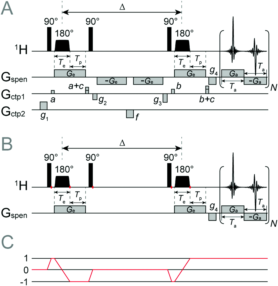

Fig. 1 SPEN DOSY pulse sequence for (A) the real experiment executed on the NMR instrument. Gradients a to c are used for coherence selection around the chirp pulses, f is a spoiler gradient, g₁, g₂ and g₃ are balancing pulses for lock signal retention, and g₄ is the prephasing gradient. T_e, T_p and T_a are the duration of the encoding gradient, the post-chirp gradient and the acquisition gradient respectively. G_a is the amplitude of the acquisition gradient, G_e is the amplitude of the encoding gradient. Chirp pulses combined with pulsed gradients frame the diffusion delay of the stimulated echo so that the signal attenuation due to spin displacement during the diffusion delay Δ is position-dependent. (B) Simulated experiment, in which straightforward coherence selection steps had been replaced by analytical coherence selection commands (indicated by red dots) to improve the numerical performance. (C) Coherence selection diagram.

The principal advantage of the Fokker–Planck formalism here is that the diffusion operator is a part of the static background Hamiltonian. Another convenient feature is that gradient operators are presented to the user in the same algebraic style as spin operators – in Fokker–Planck space, they are matrices³³ that may either be added to the background Hamiltonian, or used with shaped pulse functions in the same way as spin operators. At the pulse sequence level, this makes the simulation code neat and easy to write. Multi-spin systems with internal interactions are also straightforward – Spinach modifies the Hamiltonian and changes all matrix dimensions as appropriate;³⁴ the pulse program code remains the same.

Fig. 2a shows the simulated free induction decay obtained for the SPEN DOSY pulse sequence. It is an echo train created by the train of gradient pulses during acquisition. In order to extract the diffusion information, the data are rearranged in the k–t space (Fig. 2b) and Fourier transformed along both dimensions (Fig. 2c). The diffusion decay curve is then obtained as a slice of the 2D matrix. When the diffusion constant is set to zero, the spatial profile (grey curve in Fig. 2d) reflects the smoothed chirp excitation profile. Otherwise (blue curve in Fig. 2d), the decay induced by the diffusion is observable in the spatial profile. The plateau of the chirp pulse can then be used for diffusion coefficient determination.

Fig. 2 SPEN DOSY simulation using the Fokker–Planck formalism. The free induction decay (A) is a series of echoes induced by the bipolar gradients. At the processing stage, it is rearranged into a matrix (B) with horizontal dimension corresponding to the t₂ evolution period, and vertical dimension to the k-space. (B). The spectrum (C) is obtained after Fourier transforms in both dimensions. The extracted diffusion profile (blue curve) and the reference signal recorded in the absence of diffusion (grey curve) are shown in (D). Physical dimensions of the sample are shown in the figure. Encoding gradients of 0.2535 T m⁻¹ were applied with a chirp pulse of 110 kHz bandwidth and a duration of 1.5 ms. The post-chirp gradient had a duration of 1.6 ms. The acquisition was performed using a train of 256 bipolar gradients, where each gradient had an amplitude of 0.52 T m⁻¹, and a duration of 192 μs and 256 points. Diffusion constant was set to 8 × 10⁻¹⁰ m² s⁻¹ (blue curve) or 0 (grey curve).

3.2 Numerical accuracy and convergence

The formalism outlined in Section 2 is exact with respect to spin dynamics: the only accuracy parameter is the time step in eqn (7), which must be sufficiently small. In the spatial dynamics part, the essential factors that influence simulation accuracy are the spatial Nyquist condition (all gradient spirals must be adequately digitised) and the accuracy of the finite difference approximation to the spatial dynamics operators, in this case diffusion. The Nyquist condition⁵⁵ is that the spatial discretisation grid must have at least two points per period of the fastest gradient spiral.

As illustrated in the left panel of Fig. 3 and in Table 1, once the Nyquist condition is satisfied, distortions disappear abruptly and excellent convergence is achieved shortly thereafter. The accuracy of the finite difference approximation is controlled by the grid point spacing and the formal accuracy order of the finite difference stencil.⁵¹ The effect of the accuracy order is illustrated, and compared to the formally exact (when the Nyquist condition is satisfied) Fourier differentiation operator in the right panel of Fig. 3. Fourier differentiation operators are very accurate, but computationally expensive because they are not sparse.

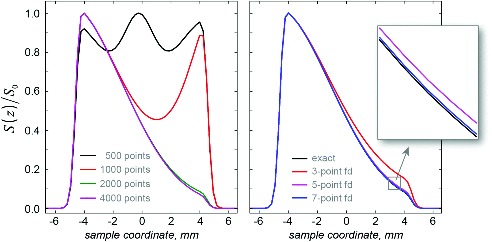Fig. 3 Left panel: the effect of the spatial Nyquist condition on the numerical accuracy of a SPEN DOSY simulation with the same physical parameters as in Fig. 2: the grids with 500 and 1000 points are sub-Nyquist and result in catastrophic loss of accuracy. Grids with 2000 points and more satisfy the Nyquist condition and produce accurate results. Right panel: the effect of the accuracy order of the finite difference approximation⁵¹ to the diffusion superoperator. The Fourier differentiation matrix (marked “exact”) is formally exact on a given grid, but has a significantly longer run time (36 minutes) compared to the much sparser finite difference matrix (less than 2 minutes).

Table 1 Convergence of the diffusion coefficient retro-fitted (using Stejskal–Tanner equation) to the simulated SPEN DOSY profile in the left panel of Fig. 3 as a function of the number of points in the spatial grid. 500-point and 1000-point grids are below the Nyquist condition for the gradient spirals. Note the linear scaling of the simulation time

Grid points	Fitted value of the diffusion coefficient, ×10^−10 m^2 s^−1	Wall clock simulation time, seconds
500	−0.07	11.6
1000	1.10	17.6
2000	7.83	33.2
3000	7.97	52.2
4000	7.98	70.0
5000	7.98	90.3

---

Practical experience indicates that periodic boundary conditions (PBC) on spatial degrees of freedom are easier to implement and simulate than absorptive or reflective boundaries. Technically, the formalism above is not restricted to periodic boundaries (finite difference operators may be built to account for other boundary types), but the implementation process is time-consuming. The use of PBC adds another accuracy consideration: for non-periodic systems, sufficient white space should be allowed on all sides of the simulation box to avoid self-interaction across the periodic boundary.

It is impossible to give a general analytical formula for the minimum number of points in the spatial grid – each pulse sequence would have its own minimal grid size. However, a convenient practical diagnostic criterion may still be formulated: the spatial Fourier transform of the Fokker–Planck state vector should not have any probability density at the high-frequency edge points at any time in the simulation.

3.3 Experimental parameter optimisation

High-fidelity numerical simulations of the SPEN DOSY pulse sequence provide useful insight into the effects of pulse sequence parameters and instrumental imperfections. An example is shown in Fig. 4 – the exact shape of the chirp pulses in Fig. 1 determines the spatial profile of the excitation region. Normalisation by the spatial profile obtained in the absence of diffusion makes it possible to retrieve a larger range of attenuations for the diffusion decay, as illustrated in Fig. 4. This also accounts for deviations from an ideal plateau due to factors like the B₁ field inhomogeneity, which is easy to model by assigning different amplitudes and directions of the control operators in eqn (2) to different voxels.

Fig. 4 Diffusion-weighted DOSY lineshape obtained under a linear gradient with (red line) and without (blue line) reference profile (grey line) correction. A significant increase in the usable signal area is evident in the background-corrected signal.

Fig. 5 shows the effect of the amplitude of the acquisition gradient G_a. It is clear that a sub-optimal choice of G_a can generate a bias (in this case, an over-estimation is produced) in the calculated diffusion constant because it yields an oscillating lineshape when decreased too much. The cause of the oscillation is signal truncation in k-space. This effect can be corrected when the reference profile is taken into account (Table 2) by dividing the diffusion profile by the reference profile computed with the diffusion coefficient set to zero. In our real experiments, a G_a of 0.20 T m⁻¹ is used; this confirms that it is necessary to correct the diffusion weighted image by a reference image with no diffusion present. Since it is impossible to switch the diffusion off in an actual experiment, the reference profile is obtained by cutting the corresponding pulses and evolution periods out of the pulse sequence in Fig. 1.

Fig. 5 The effect of gradient amplitude on the shape of the sample image in the absence of spatial diffusion (left) and with a typical diffusion constant of 8 × 10⁻¹⁰ m² s⁻¹ (right). The oscillatory distortions, called Gibbs ringing, are due to the truncation of the k-space signal.

Table 2 The effect of the acquisition gradient amplitude on the extracted diffusion coefficient (true value of 8.0 × 10⁻¹⁰ m² s⁻¹) with and without k-space truncation artefact correction

Acquisition gradient (T m^−1)	D (raw) × 10^−10 m^2 s^−1	D (corrected) × 10^−10 m^2 s^−1
0.52	7.97	7.98
0.26	7.97	7.98
0.20	8.06	7.98
0.13	8.18	7.97

---

In order to extract diffusion coefficients from the experimental SPEN DOSY data, the gradient-induced attenuation in the signal S(z) is usually fitted by the modified Stejskal–Tanner equation:⁵⁴

where D is the diffusion coefficient, Δ is the diffusion delay, T_e is the duration of the encoding gradient, T_p is the duration of the post-chirp gradient, and K(z) is the effective gradient area at position z:where G_e is the encoding gradient amplitude, γ is the magnetogyric ratio for the nuclei in question, and the phase φ(z) imparted by the chirp pulse is:where Ω₀ is the frequency offset of the NMR signal, Ω_RF(t) is the time-dependent frequency of the RF sweep, ω_RF(t) is the time-dependent amplitude of the RF field.

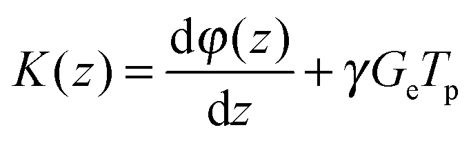
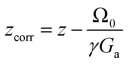
Numerical simulations are also useful in assessing the effect of chemical shift offsets on the errors in the fitting of eqn (12) to the experimental SPEN DOSY data. Chemical shifts cause two types of signal displacements. The displacement upon encoding is accounted for in eqn (14), but the chemical shift displacement during acquisition also has to be taken into account, as it may otherwise result in significant errors. Fig. 6 shows the spatial diffusion profiles obtained for several values of the chemical shift offset, and Table 3 gives the corresponding fitted values of the diffusion coefficients, for corrected and uncorrected z values in eqn (12), with

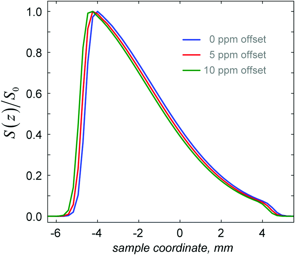Fig. 6 Simulated diffusion profile displacement for three different chemical shift offsets of the working signal from the resonance frequency. All other parameters are as in Fig. 3–5.

Table 3 Diffusion coefficients extracted from raw and corrected DOSY profiles for different values of NMR signal offset from the resonance

Chemical shift (ppm)	D (raw) × 10^−10 m^2 s^−1	D (corrected) × 10^−10 m^2 s^−1
0	7.97	7.97
5	7.73	7.97
10	7.52	7.97

---

For typical proton chemical shifts and gradient amplitudes of the same order as in Table 2, the chemical shift offset error in the diffusion coefficient is of the order of 5%; the decision on whether this is significant rests with the user, but eqn (15) is in any case straightforward to apply.

5. Quantum mechanical processes

An emerging class of MRI experiments that essentially requires quantum mechanical treatment of spin processes is singlet state imaging.^27,56,57 One reason is the delicate interplay of symmetry, chemical shift anisotropy and dipolar coupling in the relaxation superoperator that makes the two-spin singlet state long-lived.⁵⁸ The other is the M2S and S2M pulse sequences that rely on the J-coupling to get the spin system in and out of the singlet state.⁵⁹ Accurate Liouville space description of the spin dynamics⁶⁰ is therefore essential. At the same time, recent proposals for using singlet states as a delivery vehicle for hyperpolarisation in MRI^27,56,61 make it necessary to include chemical kinetics, diffusion, and flow.

In this situation, the Fokker–Planck equation is clearly superior to the more traditional Liouville–von Neumann equation formalism because all spatial dynamics processes (diffusion, hydrodynamics, magic angle spinning, spatially selective pulses, etc.) are represented by constant matrices that are more convenient from the programming and numerical efficiency point of view than the time-dependent Hamiltonians in the Liouville–von Neumann formalism.³³

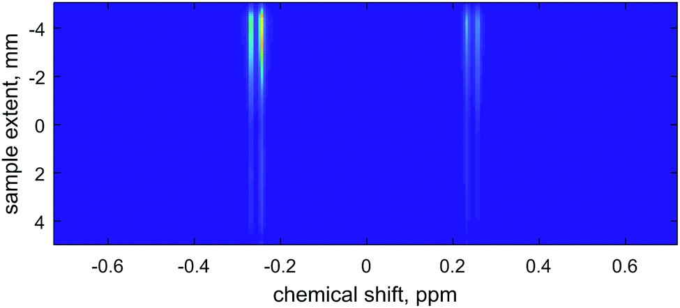
A simulation of the singlet state diffusion and flow experiment from Fig. 2 of the recent paper by Pileio et al.²⁷ shown in Fig. 7 is a particularly good example, because all of the complexities – shaped pulses, gradients, diffusion, flow, quantum mechanical spin evolution and complicated relaxation theory – are present simultaneously. An average over 100 000 Monte-Carlo instances had to be performed by the authors of the original paper, with only statistical guarantees of convergence;²⁷ here we demonstrate that the Fokker–Planck formalism performs the same simulation deterministically in a single run.

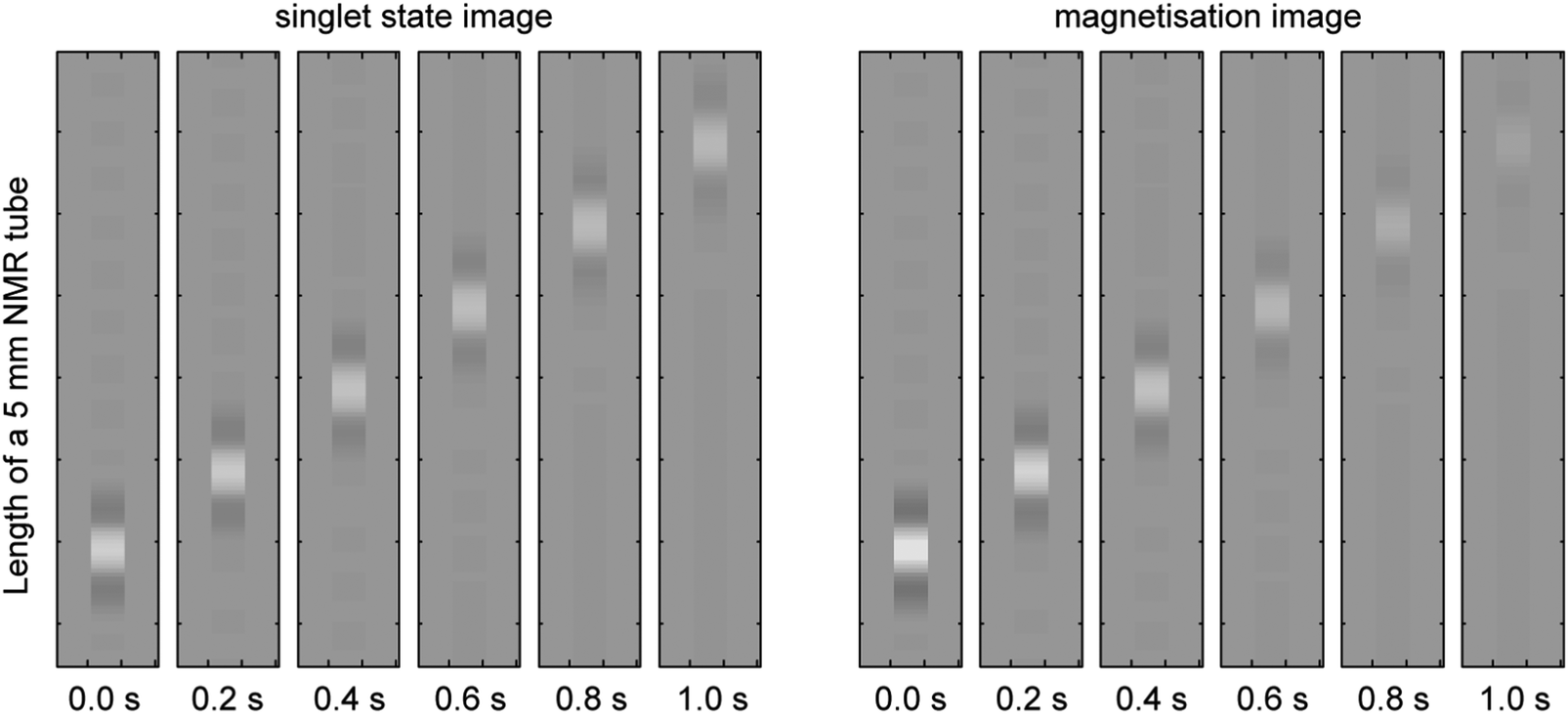Fig. 7 Fokker–Planck theory simulation of a singlet state NMR imaging experiment in the presence of diffusion and flow. The simulation includes soft radiofrequency pulses with simultaneous explicit simulation of flow, diffusion, magnetic field gradients and spin–spin coupling dynamics as prescribed by the Liouville–von Neumann equation, as well as full Redfield relaxation superoperator treatment. The flow rate is set to 5 cm s⁻¹ and the diffusion coefficient to 3.6 × 10⁻⁶ m² s⁻¹. The singlet imaging sequence used is described in a recent paper from the Pileio group.²⁷ It is clear that the very slowly relaxing singlet state flow (left panels) can be tracked at longer distances than magnetisation flow (right panels).

Fig. 8 illustrates the same point – within the Fokker–Planck formalism, diffusion and imaging simulations for systems with multiple coupled spins can be carried out in exactly the same way as for uncoupled spins – eqn (1) supports arbitrary spin Hamiltonian commutation superoperators, arbitrary relaxation theories and a host of other processes, such as chemical kinetics.

Fig. 8 A simulated ultrafast DOSY spectrum for a two-proton spin system at 600 MHz with diffusion (8 × 10⁻¹⁰ m² s⁻¹), flow (0.1 mm s⁻¹), chemical shift difference (0.5 ppm), strong J-coupling (15 Hz), full Redfield DD-CSA relaxation superoperator (2.5 Angstrom, CSA eigenvalues [−10 −10 20] ppm on both spins, with the tensor on spin 1 being collinear to the distance vector and the tensor on spin 2 being perpendicular to it, rotational correlation time 1.0 ns), and a non-symmetric chemical exchange process between the two spins (k₊ = 5 Hz, k₋ = 10 Hz). The calculation was set up in ten minutes and took less than five minutes to run with 3000 discretisation points in the spatial grid.

6. Conclusions and outlook

It is demonstrated above that NMR and MRI experiments with elaborate spatial encoding and complicated spatial dynamics are no longer hard to simulate, even in the presence of spin–spin couplings and exotic relaxation effects, such as singlet state symmetry lockout. Versions 1.10 and later of Spinach library³⁴ support arbitrary stationary flows and arbitrary distributions of anisotropic diffusion tensors in three dimensions simultaneously with Liouville-space description of spin dynamics, chemical kinetics and relaxation processes. The key simulation design decision that has made this possible is the abandonment of the Bloch–Torrey^20,21 and Liouville–von Neumann^13,35 formalisms in favour of the Fokker–Planck equation.³³ The primary factors that have facilitated this transition are the dramatic recent improvement in the speed and capacity of digital computers, the emergence of transparent and convenient sparse matrix manipulation methods in numerical linear algebra,⁶² and the recent progress in matrix dimension reduction in magnetic resonance simulations.^34,47

In the more distant perspective, high-fidelity simulations that are free of significant approximations are expected to play an increasing role in magnetic resonance experiment design and in subsequent data processing. As optimal control theory^63,64 illustrates, the understanding of the detailed dynamics taking place in a particular experiment is increasingly hard to achieve; it is slowly being replaced by the understanding of the factors generating the dynamics. Mathematically, this corresponds to the well-known relationship between a Lie group – usually an exceedingly complicated object – and the Lie algebra of its generators, which is fundamentally easier to understand and interpret. For complicated systems and processes, numerical simulation is the only practical way of connecting the two.

Acknowledgements

This research was supported by the Région Ile-de-France, by a CNRS – Royal Society exchange scheme, EPSRC (EP/M003019/1), and by the Agence Nationale de la Recherche (ANR-16-CE29-0012). The authors are indebted to Giuseppe Pileio, Maria Grazia Concilio, Gareth Morris, Lucio Frydman, Davy Sinnaeve and Mohammadali Foroozandeh for stimulating discussions. The authors also acknowledge the use of the IRIDIS High Performance Computing Facility, and associated support services at the University of Southampton, in the completion of this work.

References

1. L. Frydman, T. Scherf and A. Lupulescu, The acquisition of multidimensional NMR spectra within a single scan, Proc. Natl. Acad. Sci. U. S. A., 2002, 99, 15858–15862.
2. Z. D. Pardo, G. L. Olsen, M. E. Fernandez-Valle, L. Frydman, R. Martinez-Alvarez and A. Herrera, Monitoring mechanistic details in the synthesis of pyrimidines via real-time, ultrafast multidimensional NMR spectroscopy, J. Am. Chem. Soc., 2012, 134, 2706–2715.
3. M. Gal, T. Kern, P. Schanda, L. Frydman and B. Brutscher, An improved ultrafast 2D NMR experiment: towards atom-resolved real-time studies of protein kinetics at multi-Hz rates, J. Biomol. NMR, 2009, 43, 1–10.
4. P. Schanda, E. Kupce and B. Brutscher, SOFAST-HMQC experiments for recording two-dimensional heteronuclear correlation spectra of proteins within a few seconds, J. Biomol. NMR, 2005, 33, 199–211.
5. P. Giraudeau and L. Frydman, Ultrafast 2D NMR: an emerging tool in analytical spectroscopy, Annu. Rev. Anal. Chem., 2014, 7, 129–161.
6. R. Schmidt and L. Frydman, New spatiotemporal approaches for fully refocused, multislice ultrafast 2D MRI, Magn. Reson. Med., 2014, 71, 711–722.
7. K. Zangger and H. Sterk, Homonuclear Broadband-Decoupled NMR Spectra, J. Magn. Reson., 1997, 124, 486–489.
8. L. Paudel, R. W. Adams, P. Kiraly, J. A. Aguilar, M. Foroozandeh, M. J. Cliff, M. Nilsson, P. Sandor, J. P. Waltho and G. A. Morris, Simultaneously enhancing spectral resolution and sensitivity in heteronuclear correlation NMR spectroscopy, Angew. Chem., 2013, 52, 11616–11619.
9. P. Giraudeau and S. Akoka, Sensitivity losses and line shape modifications due to molecular diffusion in continuous encoding ultrafast 2D NMR experiments, J. Magn. Reson., 2008, 195, 9–16.
10. Y. Shrot and L. Frydman, The effects of molecular diffusion in ultrafast two-dimensional nuclear magnetic resonance, J. Chem. Phys., 2008, 128, 164513.
11. I. Kuprov, Fokker–Planck formalism in magnetic resonance simulations, J. Magn. Reson., 2016, 270, 124–135.
12. P. A. Hardy, R. M. Henkelman, J. E. Bishop, E. C. S. Poon and D. B. Plewes, Why fat is bright in rare and fast spin-echo imaging, J. Magn. Reson. Imaging, 1992, 2, 533–540.
13. L. Stables, R. Kennan, A. Anderson and J. Gore, Density matrix simulations of the effects of J coupling in spin echo and fast spin echo imaging, J. Magn. Reson., 1999, 140, 305–314.
14. A. M. Stokes, Y. Feng, T. Mitropoulos and W. S. Warren, Enhanced refocusing of fat signals using optimized multipulse echo sequences, Magn. Reson. Med., 2013, 69, 1044–1055.
15. S. J. Nelson, J. Kurhanewicz, D. B. Vigneron, P. E. Larson, A. L. Harzstark, M. Ferrone, M. van Criekinge, J. W. Chang, R. Bok and I. Park, Metabolic imaging of patients with prostate cancer using hyperpolarized [1-13C] pyruvate, Sci. Transl. Med., 2013, 5, RA108.
16. G. Pileio, S. Bowen, C. Laustsen, M. C. Tayler, J. T. Hill-Cousins, L. J. Brown, R. C. Brown, J. H. Ardenkjaer-Larsen and M. H. Levitt, Recycling and imaging of nuclear singlet hyperpolarization, J. Am. Chem. Soc., 2013, 135, 5084–5088.
17. L. Frydman, A. Lupulescu and T. Scherf, Principles and features of single-scan two-dimensional NMR spectroscopy, J. Am. Chem. Soc., 2003, 125, 9204–9217.
18. S. Yang, J. Lee, E. Joe, H. Lee, Y.-S. Choi, J. M. Park, D. Spielman, H.-T. Song and D.-H. Kim, Metabolite-selective hyperpolarized 13C imaging using extended chemical shift displacement at 9.4 T, Magn. Reson. Imaging, 2016, 34, 535–540.
19. P. K. Senanayake, N. J. Rogers, K. L. N. Finney, P. Harvey, A. M. Funk, J. I. Wilson, D. O'Hogain, R. Maxwell, D. Parker and A. M. Blamire, A new paramagnetically shifted imaging probe for MRI, Magn. Reson. Med., 2016, 77, 1307–1317.
20. T. H. Jochimsen, A. Schäfer, R. Bammer and M. E. Moseley, Efficient simulation of magnetic resonance imaging with Bloch–Torrey equations using intra-voxel magnetization gradients, J. Magn. Reson., 2006, 180, 29–38.
21. D. V. Nguyen, J.-R. Li, D. Grebenkov and D. Le Bihan, A finite elements method to solve the Bloch–Torrey equation applied to diffusion magnetic resonance imaging, J. Comput. Phys., 2014, 263, 283–302.
22. H. Benoit-Cattin, G. Collewet, B. Belaroussi, H. Saint-Jalmes and C. Odet, The SIMRI project: a versatile and interactive MRI simulator, J. Magn. Reson., 2005, 173, 97–115.
23. D. A. Yoder, Y. Zhao, C. B. Paschal and J. M. Fitzpatrick, MRI simulator with object-specific field map calculations, Magn. Reson. Imaging, 2004, 22, 315–328.
24. J. S. Petersson, J. O. Christoffersson and K. Golman, MRI simulation using the k-space formalism, Magn. Reson. Imaging, 1993, 11, 557–568.
25. T. Stöcker, K. Vahedipour, D. Pflugfelder and N. J. Shah, High-performance computing MRI simulations, Magn. Reson. Med., 2010, 64, 186–193.
26. P. T. Callaghan, A Simple Matrix Formalism for Spin Echo Analysis of Restricted Diffusion under Generalized Gradient Waveforms, J. Magn. Reson., 1997, 129, 74–84.
27. G. Pileio, J.-N. Dumez, I.-A. Pop, J. T. Hill-Cousins and R. C. D. Brown, Real-space imaging of macroscopic diffusion and slow flow by singlet tagging MRI, J. Magn. Reson., 2015, 252, 130–134.
28. C. Cai, M. Lin, Z. Chen, X. Chen, S. Cai and J. Zhong, SPROM – an efficient program for NMR/MRI simulations of inter- and intra-molecular multiple quantum coherences, C. R. Phys., 2008, 9, 119–126.
29. A. D. Fokker, Die mittlere Energie rotierender elektrischer Dipole im Strahlungsfeld, Ann. Phys., 1914, 348, 810–820.
30. M. Planck, Über einen Satz der statistischen Dynamik und seine Erweiterung in der Quantentheorie, Sitzungsber. K. Preuss. Akad. Wiss., 1917, 324–341.
31. H. Risken, The Fokker–Planck Equation, Springer, 1984.
32. L. J. Edwards, D. V. Savostyanov, A. A. Nevzorov, M. Concistrè, G. Pileio and I. Kuprov, Grid-free powder averages: On the applications of the Fokker–Planck equation to solid state NMR, J. Magn. Reson., 2013, 235, 121–129.
33. I. Kuprov, Fokker–Planck formalism in magnetic resonance simulations, J. Magn. Reson., 2016, 270, 124–135.
34. H. Hogben, M. Krzystyniak, G. Charnock, P. Hore and I. Kuprov, Spinach – a software library for simulation of spin dynamics in large spin systems, J. Magn. Reson., 2011, 208, 179–194.
35. R. R. Ernst, G. Bodenhausen and A. Wokaun, Principles of nuclear magnetic resonance in one and two dimensions, Clarendon Press Oxford, 1987.
36. G. Moro and J. H. Freed, Efficient computation of magnetic resonance spectra and related correlation functions from stochastic Liouville equations, J. Phys. Chem., 1980, 84, 2837–2840.
37. A. Polimeno and J. H. Freed, A many-body stochastic approach to rotational motions in liquids, Adv. Chem. Phys., 1993, 83, 89.
38. M. Goldman, Formal theory of spin–lattice relaxation, J. Magn. Reson., 2001, 149, 160–187.
39. A. G. Redfield, On the theory of relaxation processes, IBM J. Res. Dev., 1957, 1, 19–31.
40. R. K. Wangsness and F. Bloch, The dynamical theory of nuclear induction, Phys. Rev., 1953, 89, 728.
41. J. H. Freed, G. V. Bruno and C. F. Polnaszek, Electron spin resonance line shapes and saturation in the slow motional region, J. Phys. Chem., 1971, 75, 3385–3399.
42. D. Goodwin and I. Kuprov, Auxiliary matrix formalism for interaction representation transformations, optimal control, and spin relaxation theories, J. Chem. Phys., 2015, 143, 084113.
43. I. Kuprov, Diagonalization-free implementation of spin relaxation theory for large spin systems, J. Magn. Reson., 2011, 209, 31–38.
44. D. Tannor, Introduction to Quantum Dynamics: A Time-Dependent Perspective, University Science Books, Sausalito, CA, 2007.
45. R. B. Sidje, Expokit: a software package for computing matrix exponentials, ACM Trans. Math. Software, 1998, 24, 130–156.
46. C. Moler and C. Van Loan, Nineteen dubious ways to compute the exponential of a matrix, SIAM Rev., 1978, 20, 801–836.
47. L. J. Edwards, D. V. Savostyanov, Z. T. Welderufael, D. Lee and I. Kuprov, Quantum mechanical NMR simulation algorithm for protein-size spin systems, J. Magn. Reson., 2014, 243, 107–113.
48. D. M. Brink and G. R. Satchler, Angular momentum, Oxford University Press on Demand, 1993.
49. A. Karabanov, I. Kuprov, G. Charnock, A. van der Drift, L. J. Edwards and W. Köckenberger, On the accuracy of the state space restriction approximation for spin dynamics simulations, J. Chem. Phys., 2011, 135, 084106.
50. L. N. Trefethen, Spectral methods in MATLAB, Siam, 2000.
51. B. Fornberg, Generation of finite difference formulas on arbitrarily spaced grids, Math. Comput., 1988, 51, 699–706.
52. T. Liszka and J. Orkisz, The finite difference method at arbitrary irregular grids and its application in applied mechanics, Comput. Struct., 1980, 11, 83–95.
53. R. Eymard, T. Gallouët and R. Herbin, Finite volume methods, Handbook of Numerical Analysis, Elsevier, 2000, pp. 713–1018.
54. L. Guduff, I. Kuprov, C. van Heijenoort and J. Dumez, Spatially encoded 2D and 3D diffusion-ordered NMR spectroscopy, Chem. Commun., 2016, 53, 701–704.
55. H. Nyquist, Certain topics in telegraph transmission theory, Trans. Am. Inst. Electr. Eng., 1928, 47, 617–644.
56. C. Laustsen, G. Pileio, M. C. D. Tayler, L. J. Brown, R. C. D. Brown, M. H. Levitt and J. H. Ardenkjaer-Larsen, Hyperpolarized singlet NMR on a small animal imaging system, Magn. Reson. Med., 2012, 68, 1262–1265.
57. J.-N. Dumez, J. T. Hill-Cousins, R. C. D. Brown and G. Pileio, Long-lived localization in magnetic resonance imaging, J. Magn. Reson., 2014, 246, 27–30.
58. G. Pileio, Relaxation theory of nuclear singlet states in two spin-1/2 systems, Prog. Nucl. Magn. Reson. Spectrosc., 2010, 56, 217–231.
59. G. Pileio, M. Carravetta and M. H. Levitt, Storage of nuclear magnetization as long-lived singlet order in low magnetic field, Proc. Natl. Acad. Sci. U. S. A., 2010, 107, 17135–17139.
60. A. D. Bain and J. S. Martin, FT NMR of nonequilibrium states of complex spin systems. I. A Liouville space description, J. Magn. Reson., 1978, 29, 125–135.
61. G. Pileio, S. Bowen, C. Laustsen, M. C. D. Tayler, J. T. Hill-Cousins, L. J. Brown, R. C. D. Brown, J. H. Ardenkjaer-Larsen and M. H. Levitt, Recycling and Imaging of Nuclear Singlet Hyperpolarization, J. Am. Chem. Soc., 2013, 135, 5084–5088.
62. J. R. Bunch and D. J. Rose, Sparse matrix computations, Academic Press, 2014.
63. P. De Fouquieres, S. Schirmer, S. Glaser and I. Kuprov, Second order gradient ascent pulse engineering, J. Magn. Reson., 2011, 212, 412–417.
64. I. Kuprov, Spin system trajectory analysis under optimal control pulses, J. Magn. Reson., 2013, 233, 107–112.

---