Ab initio calculation of inelastic scattering
Received
30th March 2017
, Accepted 26th April 2017
First published on 26th April 2017
Abstract
Nonresonant inelastic electron and X-ray scattering cross sections for bound-to-bound transitions in atoms and molecules are calculated directly from ab initio electronic wavefunctions. The approach exploits analytical integrals of Gaussian-type functions over the scattering operator, which leads to accurate and efficient calculations. The results are validated by comparison to analytical cross sections in H and He+, and by comparison to experimental results and previous theory for closed-shell He and Ne atoms, open-shell C and Na atoms, and the N2 molecule, with both inner-shell and valence electronic transitions considered. The method is appropriate for use in conjunction with quantum molecular dynamics simulations and for the analysis of new ultrafast X-ray scattering experiments.
1 Introduction
X-ray scattering has been, and continues to be, instrumental for investigations into the properties of matter. While elastic scattering plays a key role in determining the structure of matter,1 inelastic scattering enables studies of dynamic properties such as the dispersion of phonons, valence electron excitations, and time-dependent electron dynamics.2 Recently, new double-differential, high energy-resolution X-ray scattering measurements at synchrotrons have begun to provide an increasingly detailed picture of electronic structure and dynamics in gas-phase atoms and molecules.3–12 One particular strength of inelastic X-ray scattering (IXS) is the ability to access optically forbidden transitions.
New X-ray Free-Electron Lasers (XFELs), in turn, generate high intensity and short duration pulses13–19 that enable time-resolved X-ray scattering,20–25 and thus ultrafast imaging of photochemical dynamics.26 An attractive feature of such experiments is that they provide direct access to the evolution of molecular geometry via the elastic scattering.27 However, questions remain regarding the degree to which inelastic contributions to the scattering signal can be ignored when analysing experiments, especially in regions where the separation of different electronic states is small.28–31 For instance, the inelastic contributions are known to be important for imaging of electronic wavepackets in atoms.32–35 A full theoretical analysis of ultrafast X-ray scattering, beyond the conventional elastic approximation, will require matrix elements corresponding to IXS,31 which provides an important incentive for the work presented in this article. In addition, it is conceivable that once the appropriate theoretical and computational tools for a more detailed analysis of ultrafast X-ray scattering experiments are in place, more detailed information can be extracted regarding the electron dynamics that accompanies the structural dynamics of a photochemical process.
In the following, we outline a method for the calculation of IXS from ab initio electronic structure calculations in atoms and molecules, based on our previously developed code for the prediction of elastic X-ray scattering.36–38 An important objective is to match the level of accuracy required for quantum molecular dynamics simulations of photochemical reactions,31 which generally implies a high-level multiconfigurational description of the electronic structure (e.g. CASSCF, CASPT2, or MRCI), while not quite reaching the level of sophistication possible when evaluating IXS from atomic targets or very small molecules (e.g. R-matrix theory) in order to maintain a necessary degree of computational efficiency. In the following, we will outline the theory, present our computational approach, and demonstrate that we can calculate IXS accurately.
2 Theory
2.1 X-ray scattering
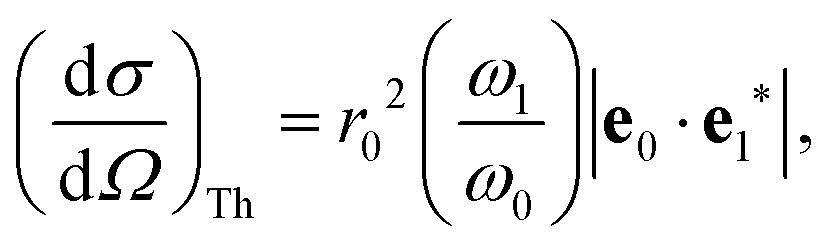
The total double differential cross section for X-ray scattering is,2| | 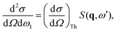 | (1) |
where the strength of the photon–electron coupling is given by the Thomson cross section,| | 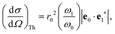 | (2) |
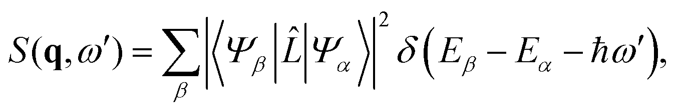
with r0 = e2/mc2 known as the classical electron radius (e is the charge of an electron and c the speed of light), ω1 and ω0 the angular frequencies of the scattered and incident X-rays, and |e0·e1*| the polarization factor. The so-called dynamic structure factor, S(q,ω′), describes the material response,| | 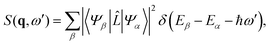 | (3) |
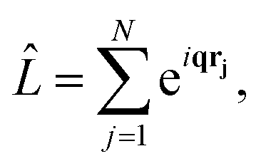
where |Ψβ〉 and |Ψα〉 are the final and initial states, ω′ = ω0 − ω1, and ![[L with combining circumflex]](https://www.rsc.org/images/entities/i_char_004c_0302.gif) is the scattering operator,
is the scattering operator,| |  | (4) |
with the sum running over all N electrons. The momentum transfer vector, q = k0 − k1, is defined as the difference between the incident and the scattered wave vectors, with k0 = k1 + ω′/c, and ħω′ = Eβ − Eα the transition energy, which often is negligible compared to the energy of hard X-rays.39
The matrix elements Lβα = 〈Ψβ||Ψα〉 in eqn (3) originate from the ![[A with combining right harpoon above (vector)]](https://www.rsc.org/images/entities/b_char_0041_20d1.gif) · terms in the interaction Hamiltonian,2 where is the vector potential of the electromagnetic field, at first order of perturbation theory. The competing contributions from the
· terms in the interaction Hamiltonian,2 where is the vector potential of the electromagnetic field, at first order of perturbation theory. The competing contributions from the ![[p with combining right harpoon above (vector)]](https://www.rsc.org/images/entities/b_char_0070_20d1.gif) terms in the Hamiltonian, which for scattering appear in second order, are sufficiently small to be disregarded.40 Diagonal matrix elements, Lαα = 〈Ψα||Ψα〉, correspond to elastic scattering and are equivalent to the Fourier transform of the target electron density, a circumstance that underpins the role of elastic scattering in structure determination.1 Further details regarding the calculation of elastic scattering from ab initio wavefunctions can be found in ref. 36 and 41. The remaining off-diagonal, α ≠ β, matrix elements correspond to nonresonant IXS, also referred to as Compton scattering, and are the focus of this article. The elastic and inelastic matrix elements for X-ray scattering, Lβα, are a necessary ingredient in detailed treatments of ultrafast X-ray scattering from non-stationary quantum states by coherent X-ray sources such as XFELs, see e.g.ref. 31, and the requirement for these matrix elements is one of the motivations for the work presented in this article.
terms in the Hamiltonian, which for scattering appear in second order, are sufficiently small to be disregarded.40 Diagonal matrix elements, Lαα = 〈Ψα||Ψα〉, correspond to elastic scattering and are equivalent to the Fourier transform of the target electron density, a circumstance that underpins the role of elastic scattering in structure determination.1 Further details regarding the calculation of elastic scattering from ab initio wavefunctions can be found in ref. 36 and 41. The remaining off-diagonal, α ≠ β, matrix elements correspond to nonresonant IXS, also referred to as Compton scattering, and are the focus of this article. The elastic and inelastic matrix elements for X-ray scattering, Lβα, are a necessary ingredient in detailed treatments of ultrafast X-ray scattering from non-stationary quantum states by coherent X-ray sources such as XFELs, see e.g.ref. 31, and the requirement for these matrix elements is one of the motivations for the work presented in this article.
There is an immediate link between IXS and inelastic scattering of fast charged particles, such as electrons, which has been exploited extensively in Electron Energy-Loss Spectroscopy (EELS).42 The inelastic scattering of electrons is described by the same matrix elements as IXS,43,44 although the approximations involved are more severe for electrons than X-rays.45 Formally, eqn (1) pertains to electron scattering if the Thomson differential cross section, (dI/dΩ)Th, is replaced by the corresponding Rutherford cross section, (dI/dΩ)Ru. The scattering elements for elastic electron scattering are not quite identical to X-ray scattering, since they contain additional contributions from electron-nuclei scattering.
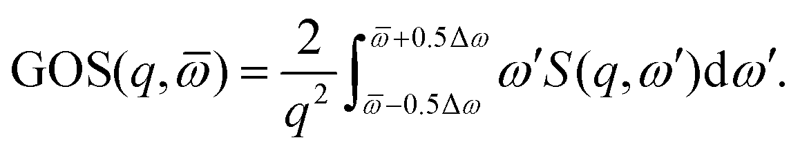
The similarity between electron and X-ray scattering in the first Born approximation can be emphasized by the use of generalised oscillator strengths (GOS).44 In brief, the GOS renormalizes the spectra using the Bethe f-sum rule,43
| | 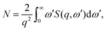 | (5) |
where
N is the number of electrons. Such renormalization provides an unitless measure of the strength of spectral features, at a given energy resolution Δ
ω, as,
| | 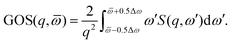 | (6) |
The GOS is often rotationally averaged to account for lack of alignment in the experiments,
44 which explains the usage of
q rather than
q in
eqn (5) and (6) above. In the literature, a sum over the final degenerate substates and an average over initial Boltzmann-weighted states is frequently implied.
2.2 Scattering matrix elements
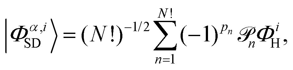
An accurate description of excited electronic states in atoms and molecules requires a multiconfiguration expansion of the wavefunction. Simple versions of the one-electron approximation for inelastic scattering are insufficient to describe Compton scattering and multielectron correlation effects must therefore, at least to some extent, be accounted for.46 In multiconfigurational ab initio electronic structure theory the valence electrons are distributed over molecular orbitals in an active space which consists of multiple electron configurations represented by Slater determinants. An electronic state, |Ψα〉, can be expanded as,| | 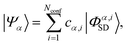 | (7) |
where the cα,i are the configuration interaction coefficients for the electronic state α, Nconf is the number of configurations included in the expansion, and |Φα,iSD〉 are the Slater determinants. The Slater determinants are given by,| | 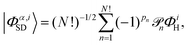 | (8) |
with ![[scr P, script letter P]](https://www.rsc.org/images/entities/char_e52f.gif) n the pair-wise permutation operator acting on the Hartree product ΦiH = χi1(q1)…χiN(qNe) where qj = (rj,ωj). The spin orbitals χij(qj) are the products of the spin functions, |↑〉 or |↓〉, and the orthonormal spatial molecular orbitals, ϕj(rj), used to construct each Slater determinant.†
n the pair-wise permutation operator acting on the Hartree product ΦiH = χi1(q1)…χiN(qNe) where qj = (rj,ωj). The spin orbitals χij(qj) are the products of the spin functions, |↑〉 or |↓〉, and the orthonormal spatial molecular orbitals, ϕj(rj), used to construct each Slater determinant.†
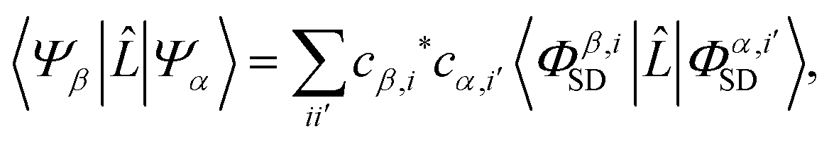
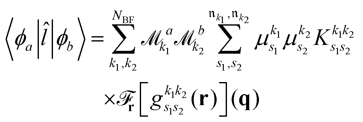
Scattering matrix elements Lβα between electronic states β and α are thus given by,
| | 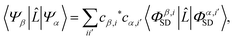 | (9) |
using the scattering operator
from
eqn (4). It is worth noting that we do not explicitly decompose the matrix elements into multipole components by applying the Wigner–Eckart theorem to the operator
in
eqn (4). The multipole expansion has the advantage that it makes it possible to derive selection rules for single atoms
46 or diatomic molecules,
47 but confers significantly less advantage in the general, non-symmetric, case. Importantly, the current treatment has the advantage that the full physical value of the matrix element is obtained straight away.
To evaluate the matrix elements, we note that is the sum of one-electron operators, leading to three standard cases for the evaluation of the brackets on the right-hand side of eqn (9).48 The first case occurs if the two Slater determinants are identical,
| | 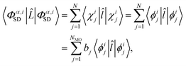 | (10) |
where
![[l with combining circumflex]](https://www.rsc.org/images/entities/i_char_006c_0302.gif)
is the single electron operator corresponding to
in
eqn (4). In the final line of
eqn (10),
bj ∈ 0, 1, 2 is the occupancy number for each spatial orbital in the Slater determinant when running the summation over all unique spatial orbitals, not just those included in that specific determinant. The second case occurs if the two Slater determinants differ by a single spin orbital when arranged in maximum coincidence,
| | 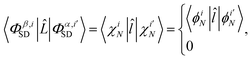 | (11) |
which is nonzero when the spins of
χiN and

are parallel, but vanishes
via 〈↓|↑〉 = 0 otherwise. Finally, if the two Slater determinants differ by more than one spin orbital, the result is always zero.
2.2.1 Evaluation of matrix elements.
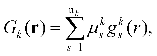
The next step requires the evaluation of the integrals that contribute to the matrix elements in eqn (3), corresponding to the brackets listed in eqn (10) and (11). These one-electron integrals over spatial orbitals, expressed in a Gaussian basis, can be evaluated analytically as outlined in the following. The molecular orbitals ϕj(rj) are obtained as linear combinations of the basis functions Gk(r),| | 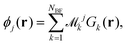 | (12) |
where ![[scr M, script letter M]](https://www.rsc.org/images/entities/char_e145.gif) jk are the molecular orbital expansion coefficients. The total number of basis functions Gk(r) is NBF, with j ∈ NMO = NBF. Each basis function Gk(r), in turn, is a contraction of Gaussian-type orbitals (GTOs), gs(r), such that,
jk are the molecular orbital expansion coefficients. The total number of basis functions Gk(r) is NBF, with j ∈ NMO = NBF. Each basis function Gk(r), in turn, is a contraction of Gaussian-type orbitals (GTOs), gs(r), such that,| | 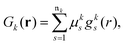 | (13) |
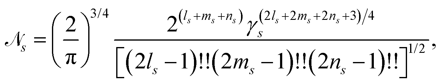
where μks are the basis set contraction coefficients for the primitive GTOs. A Cartesian Gaussian-type orbital centered at coordinates rs = (xs,ys,zs) has the form,| | gs(r) = ![[scr N, script letter N]](https://www.rsc.org/images/entities/char_e52d.gif) s(x − xs)ls(y − ys)ms(z − zs)nse−γs(r−rs)2, s(x − xs)ls(y − ys)ms(z − zs)nse−γs(r−rs)2, | (14) |
with exponent γs, Cartesian orbital angular momentum Ls = ls + ms + ns, and normalisation constant s,| |  | (15) |
where !! denotes the double factorial. The usage of Cartesian GTOs is convenient in the present context, but there is a direct mapping between Cartesian and spherical Gaussians.49 If spherical Gaussians are used the mathematics of the analytic Fourier transform takes a different form.50
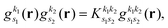
The one-electron bracket in eqn (10) and (11) can then be evaluated as,
| |  | (16) |
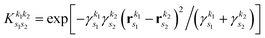
where we use the Gaussian product theorem
51 to rewrite the product

as,
| |  | (17) |
where
is the pre-factor and

is the new Gaussian centered at
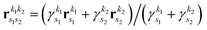
with exponent

. Since the Cartesian coordinates (
x,
y,
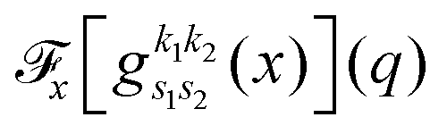
z) are linearly independent and each Gaussian function can be written as a product of
x,
y and
z components,
| |  | (18) |
the problem is reduced to the solution of one-dimensional Fourier transforms
. These can be determined analytically, as has been shown and tabulated in a previous publication.
36
3 Computational details
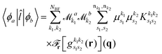
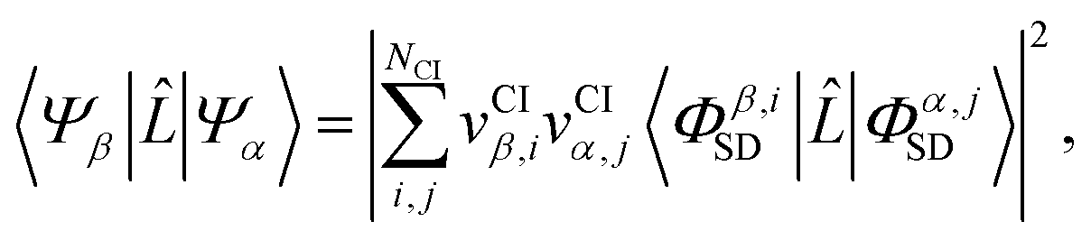
As pointed out in Section 2.2, a correct description of excited electronic states requires multiconfigurational wavefunctions. In the following, we focus on CASSCF, MCSCF, and MRCI level theory, which provides an attractive compromise between computational resources and accuracy, and constitutes a level of theory frequently used in quantum molecular dynamics simulations of small and medium sized molecules.52–55 The wave functions are calculated using state averaging and the results are expressed using CI configurations, with the weights given by the configuration interaction vector. The calculations are more convenient if the CI vector is expanded over configuration state functions (CSF) instead over individual Slater determinants. In the case of MRCI methods, the calculation is performed using CSF already, expressing the spin populations as branches with only a merely statistical meaning in terms of spin quantum numbers. This gives the inelastic scattering matrix elements as,| | 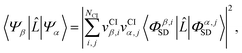 | (19) |
where vCIα are the CI-vectors of length NCI. Only pairs of Slater determinants that differ by less than two occupied orbitals will give a non-zero result, as discussed earlier, which makes it possible to swiftly filter out null contributions to the integrals. If doublet or triplet states are considered, appropriate prefactors need to be included when spatial orbitals are evaluated. Furthermore, in small systems, such as atoms or diatomic molecules, symmetry is useful to reduce the number of calculations required. We have used the electronic structure package MOLPRO56 to carry out the ab initio calculations, and calculated the IXS cross sections using a new version of our recently developed ab initio X-ray diffraction (AIXRD) code.36
The IXS cross sections in this article are given in terms of the dynamic structure factor, S(q,ωβ), or the generalized oscillator strength, GOS(q,![[small omega, Greek, macron]](https://www.rsc.org/images/entities/i_char_e0da.gif) ), with the choice between the two representations determined by the source of the reference data used for comparison. All calculated data is given at perfect energy resolution, i.e. with no averaging over energy (Δω = 0 in eqn (6)). The results for Ne and N2 are rotationally averaged to match published data. Furthermore, the astute reader will notice that some graphs show the cross sections as a function of q, while others as a function of q2. The choice, again, reflects the source of the reference data, with EELS measurements (or IXS measurements that compare to EELS data) generally shown as a function of q2 in order to offset the small angle of scattering for EELS.
), with the choice between the two representations determined by the source of the reference data used for comparison. All calculated data is given at perfect energy resolution, i.e. with no averaging over energy (Δω = 0 in eqn (6)). The results for Ne and N2 are rotationally averaged to match published data. Furthermore, the astute reader will notice that some graphs show the cross sections as a function of q, while others as a function of q2. The choice, again, reflects the source of the reference data, with EELS measurements (or IXS measurements that compare to EELS data) generally shown as a function of q2 in order to offset the small angle of scattering for EELS.
4 Results and discussion
4.1 Single-electron atoms
We begin by a comparison of analytical and numerical results for the dynamic structure factor, S(q,ω), in the single-electron atoms H and He+. The analytical results are computed along the lines in ref. 50. Numerically, the wavefunctions are calculated at the CASSCF(1,3) level, which is more than sufficient in the present case, using the Dunning basis d-aug-cc-PV5Z. The d-aug family of basis sets allows a better description of the diffuse orbitals in hydrogen-like atoms when the principal quantum number is n > 1, i.e. for hydrogenic Rydberg states. The calculated ab initio transition energies for (2s,2p,3s) ← 1s are within <0.1% of the experimental57 and analytical result. As apparent from Fig. 1, the analytical and numerical results for S(q,ω) agree well in both cases, with the dynamic structure factor extending to larger values of q for transitions for the more compact He+ states (Fig. 1b) compared to H (Fig. 1a), as expected.
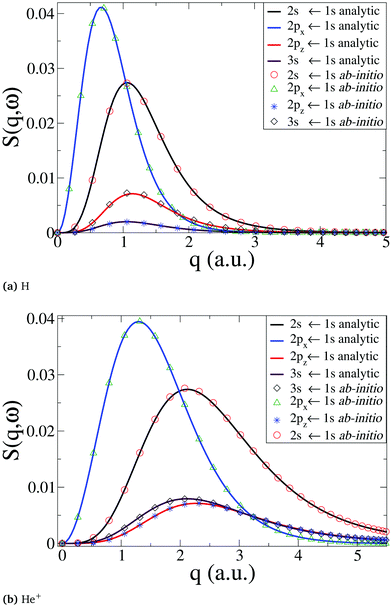 |
| | Fig. 1 Comparison between numerical ab initio calculations, using our approach, and analytical results for (a) the H neutral atom, and (b) the He+ cation. The dynamic structure factor, S(q,ω), is shown for the transitions 2s ← 1s, 2px(2py) ← 1s, 2pz ← 1s, and 3s ← 1s. | |
4.2 Two-electron atoms
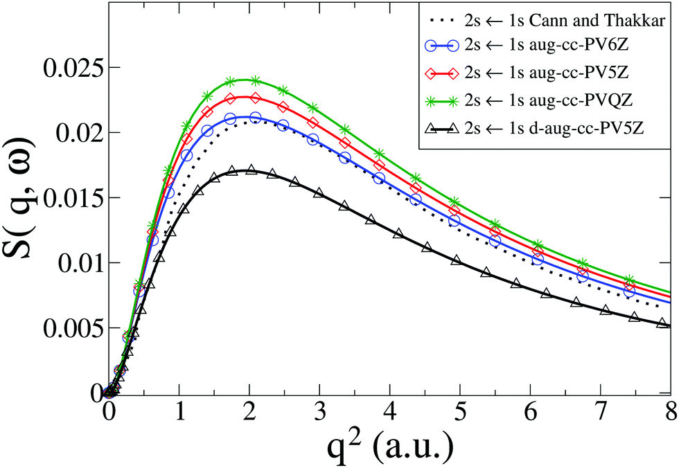
We now consider the He atom, a two-electron system. The electronic states of He are well known. The energy convergence for CASSCF(2,10) ab initio calculations with four different Dunning basis sets is shown in Table 1 for the two excited states 1S0(1s2s) and 1P1(1s2p), with the corresponding dynamic structure factor for the 1S0(1s2s) ← 1S0(1s2) transition from the ground state shown in Fig. 2 together with reference calculations using explicitly correlated wavefunctions by Cann and Thakkar.58 Agreement between the reference results and our calculations is good, with the best agreement achieved with the aug-cc-PV6Z basis, which also has the best energy convergence. The remaining discrepancies for the aug-cc-PV6Z basis occur predominantly at small values of q. Importantly, the correlation between energy convergence in Table 1 and the quality of the scattering in Fig. 2, indicate that the calculations are robust and that systematic improvements are possible. The energy convergence is a good predictor of the quality of the calculated inelastic scattering; we have previously made the same observation for the calculation of elastic scattering matrix elements.37,38
Table 1 Energies E for the 1S0(1s2s) and 1P1(1s2p) states in He calculated at the CASSCF(2,10) level with Dunning basis sets: aug-cc-PVQZ, aug-cc-PV5Z, aug-cc-PV6Z, and d-aug-cc-PV5Z. The percentage error, ΔE, compared to experimental values from NIST57 is also given
| He |
1S0(1s2s) |
1P1(1s2p) |
|
E (eV) |
ΔE (%) |
E (eV) |
ΔE (%) |
| Exp.57 |
20.615 |
— |
21.218 |
— |
| PVQZ |
20.793 |
0.8 |
23.943 |
12.8 |
| PV5Z |
20.748 |
0.6 |
23.078 |
8.8 |
| PV6Z |
20.684 |
0.3 |
22.667 |
6.8 |
| d-PV5Z |
20.000 |
3.0 |
20.680 |
2.5 |
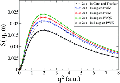 |
| | Fig. 2 Calculated dynamic structure factor, S(q,ω), in He for the 1S0(1s2s) ← 1S0(1s2) transition compared to results from Cann and Thakkar.58 The numerical calculations are performed with CASSCF(2,10) and four Dunning basis sets (aug-cc-PVQZ, aug-cc-PV5Z, aug-cc-PV6Z, and d-aug-cc-PV5Z). | |
In Fig. 3 we compare our calculated dynamic structure factors for the two transitions 1S0(1s2s) ← 1S0(1s2) and 1P1(1s2p) ← 1S0(1s2) in He to experimental results by Xie et al.7 and reference calculations by Cann and Thakkar.58 The agreement between present and previous calculations and the experimental data is good, with the reference calculations reproducing experiments slightly better for q < 2 a.u. The fact that the energy convergence for the 1S0 state is better than for the 1P1 state in our calculations (see Table 1) appears to have little effect on the agreement between the dynamic structure factor for the two transitions in our calculations and the experimental results, with the convergence of 1S0(1s2s) ← 1S0(1s2) only marginally better than for 1P1(1s2p) ← 1S0(1s2). Notably, for both transitions the best agreement with experimental data is achieved with the basis set that yields the best energy convergence for that state (see Table 1).
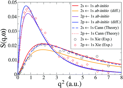 |
| | Fig. 3 Calculated dynamic structure factor, S(q,ω), in He for the 1S0(1s2s) ← 1S0(1s2) and 1P1(1s2p) ← 1S0(1s2) transitions compared to theory by Cann and Thakkar58 and experiments by Xie et al.7 The ab initio calculations are done at the CASSCF(2,10)/aug-cc-PV6Z and the CASSCF(2,10)/d-aug-cc-PV5Z levels, with the d-aug results identified by the label “(diff.)”. | |
4.3 Multi-electron atoms
4.3.1 Ne.
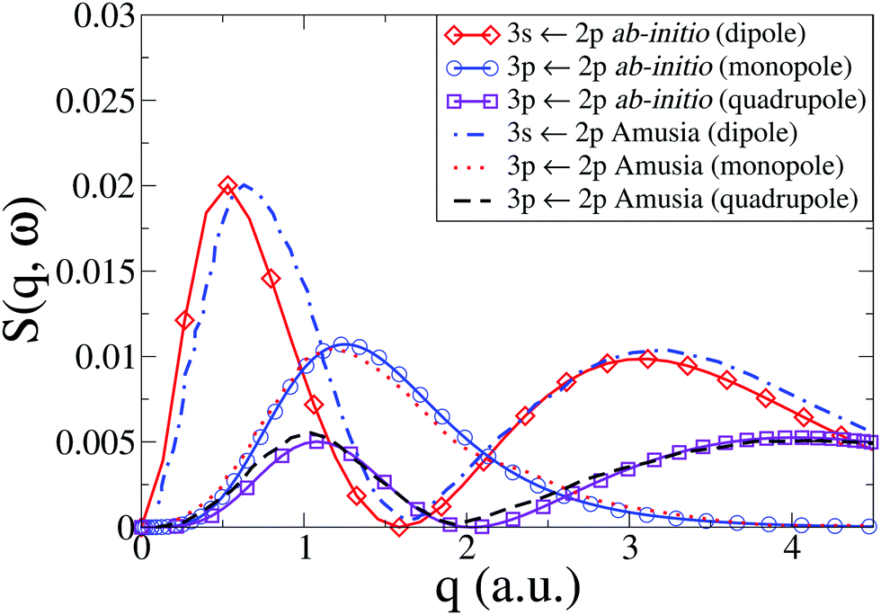
The first multi-electron atom that we consider is the closed-shell rare-gas atom Ne, where we investigate inelastic excitations from the outer subshell np6 electrons. These have been studied before, theoretically46,59 and experimentally using both EELS60 and IXS.10 The IXS measurements by Zhu et al.10 demonstrate elegantly that the intensity of the EELS measurements at high q is increased by contamination from high-order Born terms corresponding to multiple scattering. For X-ray scattering, only first-order Born terms contribute due to the weaker interaction.
In the following, we focus the comparison on the previous benchmark random-phase with exchange (RPAE) calculations by Amusia et al.46 The excitations studied are characterized by the dependency on the total angular momentum, and following the lead of Amusia et al. we discuss the cross sections in terms of the monopole, dipole, and quadrupole transitions, respectively. We perform our ab initio calculations at the CASSCF(10,9)/aug-cc-PVTZ level of theory. Note that when using a general-use ab initio electronic structure package, one has to pay careful attention to symmetry and multiplicity in order to isolate different contributions correctly for an atom. The energies of the excited states of Ne involved in the monopole, dipole, and quadrupole transitions from the ground state are listed in Table 2.
Table 2 Energies Ecalc for excited states in Ne atom calculated using CASSCF(10,9)/aug-cc-PVTZ. The percentage error, ΔE, relative experimental values Eexp from NIST57 is also given
| Ne |
E
exp (eV) |
E
calc (eV) |
ΔE (%) |
| 2s2p53s[1/2]1 |
16.715 |
16.554 |
1.0 |
| 2s2p53p[1/2]0 |
18.555 |
18.290 |
1.4 |
| 2s2p53p[3/2]2 |
18.704 |
18.720 |
0.1 |
In Fig. 4 we compare our results with those by Amusia et al.46 for the monopole and quadrupole 3p ← 2p and the dipole 3s ← 2p transitions. Note that the cross sections have been rotationally averaged (see Section 2). Overall, the agreement is very good, with the only notable discrepancy occurring for the dipole 3s ← 2p transition, where the low-q peak in our calculations is marginally shifted to lower values of q compared to Amusia et al., although the height and width of the peak agree almost perfectly. The Amusia et al. calculations have been compared to the recent IXS experiments by Zhu et al.,10 and the agreement for the monopole 2p53p[1/2]0, the dipole 2p53s[1/2]1, and the quadrupole 2p53p[5/2,3/2]2 were found to be quite good, which carries over to our present calculations.
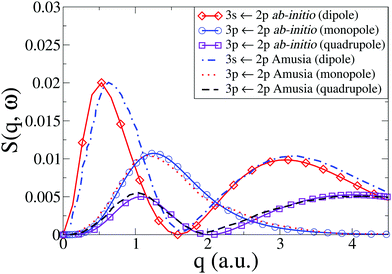 |
| | Fig. 4 Dynamic structure factor, S(q,ω), in Ne for the 3s ← 2p dipolar and 3p ← 2p monopolar and quadrupolar transitions compared to results by Amusia et al.46 | |
4.3.2 C and Na.
Next we consider two open-shell atoms, C and Na, which provides an opportunity to examine cross sections for inner shell excitations in higher multiplicity systems with unpaired electrons in the ground state and a significant degree of electron correlation. The energy convergence of the CASSCF/aug-cc-PVTZ calculations are shown in Table 3.
Table 3 Energies Ecalc for excited states in atoms C and Na calculated at the CASSCF/aug-cc-PVTZ level of theory (see text for details). The percentage error, ΔE, compared to experimental values Eexp from NIST57 and Bielschowsky et al.62 is also given
| Atom [state] |
E
exp (eV) |
E
calc (eV) |
ΔE (%) |
C [2s2p3![[thin space (1/6-em)]](https://www.rsc.org/images/entities/char_2009.gif) 3P] 3P] |
9.33057 |
9.576 |
2.6 |
| C [2s2p33D] |
7.94657 |
7.410 |
6.7 |
| Na [2p53s22P] |
31.20062 |
31.489 |
0.9 |
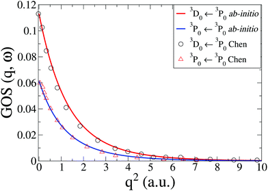
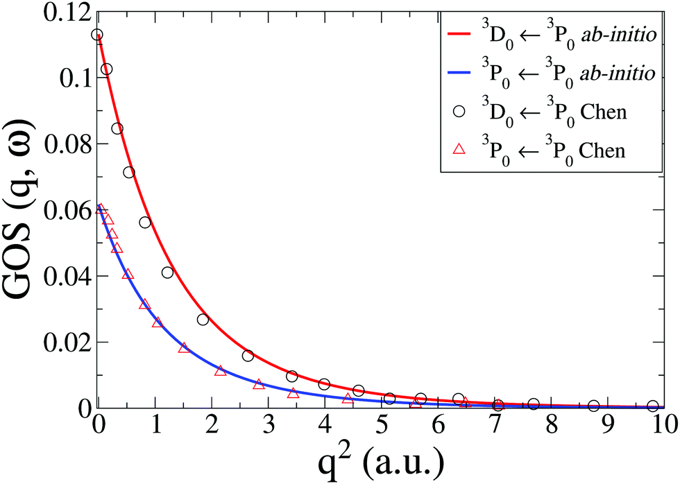
The IXS cross sections for the transitions from the ground state of the C atom to the first two inner-shell excited states, i.e.3P([He]2s2p3) ← 3P([He]2s22p2) and 3D([He]2s2p3) ← 3P([He]2s22p2), are shown in Fig. 5. Our ab initio calculations, done at the CASSCF(6,5)/aug-cc-PVTZ level, agree well with the RPAE calculations by Chen and Msezane,61 also included in Fig. 5. For q2 → 0 the GOSs should converge to the optical oscillator strength of the transitions. In our calculations these values are 0.0615 and 0.1130, respectively, which agrees reasonably well with the experimental values of 0.0634 and 0.0718,63 as well as previous theory.61 Further improvements in the oscillator strength would most likely require CASPT2 level corrections.
 |
| | Fig. 5 Generalized oscillator strengths, GOS(q,ω), in C for the two transitions 3P0(2s2p3) ← 3P0(2s22p2) and 3D0(2s2p3) ← 3P0(2s22p2). The current ab initio calculations using CASSCF(6,5)/aug-cc-PVTZ are compared to RPAE calculations by Chen and Msezane.61 | |
In Na, we have done the calculations at the CASSCF(11,9)/aug-cc-PVQZ level of theory. We consider an inner shell excitation from the doublet ground state, i.e. the 2P([He]2s22p53s2) ← 2S([He]2s22p63s) transition, which has a very low oscillator strength compared to outer electron excitations. The cross sections, shown in Fig. 6 compare well to previous theory at the HF and RPAE level61 and EELS experiments by Bielschowsky et al.62
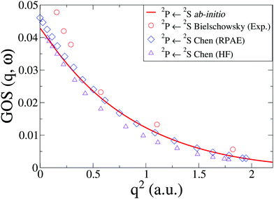 |
| | Fig. 6 The generalized oscillator strength, GOS(q,ω), in Na for the 2P(2s22p53s2) ← 2S(2s22p63s) transition. The ab initio calculations using CASSCF(11,9)/aug-cc-PVQZ are compared to experiments by Bielschowsky62 and theory by Chen and Msezane.61 | |
4.4 Molecules
Finally, we demonstrate that our codes can also calculate IXS cross sections in molecules. We consider the nitrogen molecule, N2, which is a major component in the earth atmosphere and has an important valence dipole forbidden transition at 9.3 eV that has been studied extensively.42 This quadrupole allowed transition, called the Lyman–Birge–Hopfield band, corresponds to the a1Πg ← X1Σ+g transition. Previous theoretical calculations include Tamm–Dancoff (TDA) and random-phase (RPA) approximations by Szabo and Ostlund,51 Hartree–Fock calculations by Chung and Lin,66 and more recent CAS and MRCI calculations by Giannerini et al.65 and TD-DFT by Sakko et al.67 These complement a large number of experimental studies.5,6,42,64,68
Bradley et al.5 have identified deviations from first Born approximation scattering in the EELS signal at high q by comparison to IXS, along the lines of similar observations in Ne discussed earlier. A detailed analysis of TD-DFT theory and experiments in ref. 6, shows further that the a1Πg ← X1Σ+g transition occurs in a region where there are additional contributions from the octupolar w1Δu ← X1Σ+g transition in the experimental signal, although in the following we focus on the transition to the a1Πg state.
The energy for the transition obtained using SA-CASSCF(14,12)/aug-cc-PVCTZ is within 0.3% of the experimental42 value. Table 4 shows the experimental and theoretical energies E for the a1Πg state in N2, as well as the percentage error, ΔE, compared to experimental values from Leung.42 Also included are the results for a MRCI(14,10)/aug-cc-PVCTZ calculation, which in principle should perform better than CASSCF, but due to computational problems had to be run at lower symmetry which adversely affected the energy convergence.
Table 4 Energy E for the a1Πg state in N2, corresponding to the transition energy from the X1Σ+g ground state. The experimental result is taken from Leung et al.42Ab initio CASSCF(14,12) and MRCI(14,10) results are shown, using the Dunning Rydberg-adapted aug-cc-PVCTZ basis. The percentage error, ΔE, compared to the experimental value is also given
| N2 |
E (eV) |
ΔE (%) |
| Exp.42 |
9.300 |
— |
| CASSCF(14,12) |
9.332 |
0.3 |
| MRCI(14,10) |
9.700 |
4.3 |
The generalized oscillator strength, GOS(q,ω), that we have calculated is in good agreement with the experimental results from Leung et al.42 and Barbieri et al.,64 shown in Fig. 7, as well as recent theoretical calculations by Giannerini.65 The MRCI results provide a slightly lower scattering cross section, but the difference is small. The calculated cross sections are below the experiments at high values of q. As discussed above, in terms of comparison to EELS the reason for this difference is primarily the failure of the first Born approximation in EELS. For IXS the discrepancy is smaller, and is due to additional contributions from the w1Δu state in the Lyman–Birge–Hopfield band.6
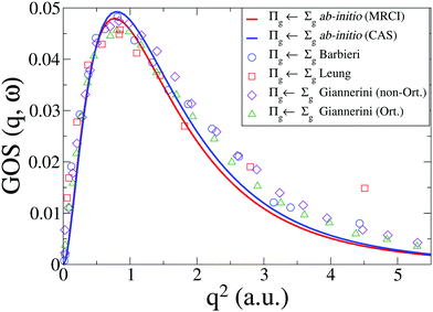 |
| | Fig. 7 Generalized oscillator strength, GOS(q,ω), for the a1Πg ← X1Σ+g transition in N2. Our CASSCF and MRCI ab initio results are compared to experimental results from Leung et al.42 and Barbieri et al.,64 and to calculations by Giannerini et al.65 | |
Finally, a brief remark regarding the energy convergence of the ab initio calculations, as summarized in Tables 1–4. In C and Na the number of Slater determinants is restricted to correctly isolate the inner-shell transitions considered, which impacts on the treatment of electron correlation. The valence transition considered in N2 allows for greater flexibility in the choice of active space, leading to a good account of static electron correlation, with the calculation close to full CI.
5 Conclusions
We have calculated a wide range of inelastic scattering cross sections, including inner-shell and valence transitions in closed and open shell atoms, and a benchmark transition in the N2 molecule. We find good agreement with experimental data from IXS and EELS, and agreement with exact theory for the H and He+ atoms and previous calculations. In terms of the Lβα off-diagonal matrix elements, a range of different computational techniques is now available. At the highly accurate end, R-matrix and RPAE based methods perform very well for calculations in single atoms, while for large systems TD-DFT strikes the necessary balance between computational cost and accuracy.67 However, TD-DFT is generally not appropriate for the simulation of complex photochemical reactions in isolated molecules, and is known to yield results that are quite divergent from established reaction paths.69
The approach presented in this paper covers the ground between these two extremes. It calculates inelastic scattering matrix elements at a level of ab initio theory congruent with state-of-the-art quantum molecular dynamics simulations, and is therefore well placed to evaluate inelastic contributions to the signals observed in ultrafast X-ray scattering experiments.31 As discussed in the Introduction, an important motivation for this work is the prospect of identifying electronic transitions in time-dependent ultrafast X-ray scattering experiments, which could enable complete characterization of reaction paths using X-ray scattering. Achieving the same insights today requires the combination of ultrafast X-ray scattering with a different experimental technique, e.g. time-resolved photoelectron spectroscopy.70 Finally, the accuracy of the matrix elements calculated by our method is only limited by the quality of the ab initio wavefunctions, and can be systematically improved by adjustments of the ab initio method and basis. Our approach involves a direct summation over all multipole matrix elements, aiding immediate comparison to experiments.
The link between IXS and EELS suggests that the codes developed here could be useful for detailed analysis of ultrafast electron diffraction (UED) data, as long as the nuclear-scattering contribution is included in the elastic terms.71 Future extensions of this work would be to include the effect of nuclear motion in the IXS signal, as we have recently done for elastic scattering,37,38 and to consider Compton ionization by the inclusion of continuum states either via multichannel quantum defect formalism72–74 or a Dyson orbital approach.75 We also aim to examine in greater detail the mapping of the wavefunction in momentum space made possible by inelastic measurements.
Acknowledgements
The authors acknowledge funding from the European Union (FP7-PEOPLE-2013-CIG-NEWLIGHT) and helpful discussions with Dr David Rogers regarding the ab initio electronic structure calculations.
References
-
D. McMorrow and J. Als-Nielsen, Elements of Modern X-Ray Physics, Wiley-Blackwell, 2nd edn, 2011 Search PubMed.
-
W. Schülke, Electron Dynamics by Inelastic X-Ray Scattering, Oxford Science Publications, 1st edn, 2007 Search PubMed.
- M. Minzer, J. A. Bradley, R. Musgrave, G. T. Seidler and A. Skilton, Rev. Sci. Instrum., 2008, 79, 086101 CrossRef CAS PubMed.
- R. Verbeni, T. Pylkkänen, S. Huotari, L. Simonelli, G. Vankó, K. Martel, C. Henriquet and G. Monaco, J. Synchrotron Radiat., 2009, 16, 469–476 CrossRef CAS PubMed.
- J. A. Bradley, G. T. Seidler, G. Cooper, M. Vos, A. P. Hitchcock, A. P. Sorini, C. Schlimmer and K. P. Nagle, Phys. Rev. Lett., 2010, 105, 053202 CrossRef CAS PubMed.
- J. A. Bradley, A. Sakko, G. T. Seidler, A. Rubio, M. Hakala, K. Hämäläinen, G. Cooper, A. P. Hitchcock, K. Schlimmer and K. P. Nagle, Phys. Rev. A: At., Mol., Opt. Phys., 2011, 84, 022510 CrossRef.
- B. Xie, L. Zhu, K. Yang, B. Zhou, N. Hiraoka, Y. Cai, Y. Yao, C. Wu, E. Wang and D. Feng, Phys. Rev. A: At., Mol., Opt. Phys., 2010, 82, 032501 CrossRef.
- L. Zhu, L. Wang, B. Xie, K. Yang, N. Hiraoka, Y. Cai and D. Feng, J. Phys. B: At., Mol. Opt. Phys., 2011, 44, 025203 CrossRef.
- X. Kang, K. Yang, Y. W. Liu, W. Q. Xu, N. Hiraoka, K. D. Tsuei, P. F. Zhang and L. F. Zhu, Phys. Rev. A: At., Mol., Opt. Phys., 2012, 86, 022509 CrossRef.
- L. F. Zhu, W. Q. Xu, K. Yang, Z. Jiang, X. Kang, B. P. Xie, D. L. Feng, N. Hiraoka and K. D. Tsuei, Phys. Rev. A: At., Mol., Opt. Phys., 2012, 85, 030501 CrossRef.
- Y.-G. Peng, X. Kang, K. Yang, X.-L. Zhao, Y.-W. Liu, X.-X. Mei, W.-Q. Xu, N. Hiraoka, K.-D. Tsuei and L.-F. Zhu, Phys. Rev. A: At., Mol., Opt. Phys., 2014, 89, 032512 CrossRef.
- Y.-W. Liu, X.-X. Mei, X. Kang, K. Yang, W.-Q. Xu, Y.-G. Peng, N. Hiraoka, K.-D. Tsuei, P.-F. Zhang and L.-F. Zhu, Phys. Rev. A: At., Mol., Opt. Phys., 2014, 89, 014502 CrossRef.
- J. N. Galayda, J. Arthur, D. F. Ratner and W. E. White, J. Opt. Soc. Am. B, 2010, 27, B106 CrossRef CAS.
- A. Barty, J. Küpper and H. N. Chapman, Annu. Rev. Phys. Chem., 2013, 64, 415 CrossRef CAS PubMed.
- C. Bostedt, J. D. Bozek, P. H. Bucksbaum, R. N. Coffee, J. B. Hastings, Z. Huang, R. W. Lee, S. Schorb, J. N. Corlett, P. Denes, P. Emma, R. W. Falcone, R. W. Schoenlein, G. Doumy, E. P. Kanter, B. Kraessig, S. Southworth, L. Young, L. Fang, M. Hoener, N. Berrah, C. Roedig and L. F. DiMauro, J. Phys. B: At., Mol. Opt. Phys., 2013, 46, 164003 CrossRef.
- J. Feldhaus, M. Krikunova, M. Meyer, T. Möller, R. Moshammer, A. Rudenko, T. Tschentscher and J. Ullrich, J. Phys. B: At., Mol. Opt. Phys., 2013, 46, 164002 CrossRef.
- M. Yabashi, H. Tanaka, T. Tanaka, H. Tomizawa, T. Togashi, M. Nagasono, T. Ishikawa, J. R. Harries, Y. Hikosaka, A. Hishikawa, K. Nagaya, N. Saito, E. Shigemasa, K. Yamanouchi and K. Ueda, J. Phys. B: At., Mol. Opt. Phys., 2013, 46, 164001 CrossRef.
- V. Lyamayev, Y. Ovcharenko, R. Katzy, M. Devetta, L. Bruder, A. LaForge, M. Mudrich, U. Person, F. Stienkemeier, M. Krikunova, T. Möller, P. Piseri, L. Avaldi, M. Coreno, P. O'Keeffe, P. Bolognesi, M. Alagia, A. Kivimäki, M. D. Fraia, N. B. Brauer, M. Drabbels, T. Mazza, S. Stranges, P. Finetti, C. Grazioli, O. Plekan, R. Richter, K. C. Prince and C. Callegari, J. Phys. B: At., Mol. Opt. Phys., 2013, 46, 164007 CrossRef.
- J. Choi, J. Y. Huang, H. S. Kang, M. G. Kim, C. M. Yim, T.-Y. Lee, J. S. Oh, Y. W. Parc, J. H. Park, S. J. Park, I. S. Ko and Y. J. Kim, J. Korean Phys. Soc., 2007, 50, 1372 CrossRef.
- M. P. Minitti, J. M. Budarz, A. Kirrander, J. S. Robinson, D. Ratner, T. J. Lane, D. Zhu, J. M. Glownia, M. Kozina, H. T. Lemke, M. Sikorski, Y. Feng, S. Nelson, K. Saita, B. Stankus, T. Northey, J. B. Hastings and P. M. Weber, Phys. Rev. Lett., 2015, 114, 255501 CrossRef CAS PubMed.
- M. P. Minitti, J. M. Budarz, A. Kirrander, J. Robinson, T. J. Lane, D. Ratner, K. Saita, T. Northey, B. Stankus, V. Cofer-Shabica, J. Hastings and P. M. Weber, Faraday Discuss., 2014, 171, 81 RSC.
- J. M. Budarz, M. P. Minitti, D. V. Cofer-Shabica, B. Stankus, A. Kirrander, J. B. Hastings and P. M. Weber, J. Phys. B: At., Mol. Opt. Phys., 2016, 49, 034001 CrossRef.
- B. Stankus, J. M. Budarz, A. Kirrander, D. Rogers, J. Robinson, T. J. Lane, D. Ratner, J. Hastings, M. P. Minitti and P. M. Weber, Faraday Discuss., 2016, 194, 525–536 RSC.
- J. M. Glownia, A. Natan, J. P. Cryan, R. Hartsock, M. Kozina, M. P. Minitti, S. Nelson, J. Robinson, T. Sato, T. van Driel, G. Welch, C. Weninger, D. Zhu and P. H. Bucksbaum, Phys. Rev. Lett., 2016, 117, 153003 CrossRef CAS PubMed.
- K. H. Kim, J. G. Kim, S. Nozawa, T. Sato, K. Y. Oang, T. W. Kim, H. Ki, J. Jo, S. Park, C. Song, T. Sato, K. Ogawa, T. Togashi, K. Tono, M. Yabashi, T. Ishikawa, J. Kim, R. Ryoo, J. Kim, H. Ihee and S. I. Adachi, Nature, 2015, 518, 385 CrossRef CAS PubMed.
- R. S. Minns and A. Kirrander, Faraday Discuss., 2016, 194, 11–13 RSC.
- R. Neutze, R. Wouts, S. Techert, J. Davidsson, M. Kocsis, A. Kirrander, F. Schotte and M. Wulff, Phys. Rev. Lett., 2001, 87, 195508 CrossRef CAS PubMed.
- N. E. Henriksen and K. B. Møller, J. Phys. Chem. B, 2008, 112, 558 CrossRef CAS PubMed.
- U. Lorenz, K. B. Møller and N. E. Henriksen, Phys. Rev. A: At., Mol., Opt. Phys., 2010, 81, 023422 CrossRef.
- K. B. Møller and N. E. Henriksen, Struct. Bonding, 2012, 142, 185 CrossRef.
- A. Kirrander, K. Saita and D. V. Shalashilin, J. Chem. Theory Comput., 2016, 12, 957–967 CrossRef CAS PubMed.
- G. Dixit, O. Vendrell and R. Santra, Proc. Natl. Acad. Sci. U. S. A., 2012, 109, 11636 CrossRef CAS PubMed.
- G. Dixit and R. Santra, J. Chem. Phys., 2013, 138, 134311 CrossRef PubMed.
- H. J. Suominen and A. Kirrander, Phys. Rev. Lett., 2014, 112, 043002 CrossRef PubMed.
- H. J. Suominen and A. Kirrander, Phys. Rev. Lett., 2014, 113, 189302 CrossRef CAS PubMed.
- T. Northey, N. Zotev and A. Kirrander, J. Chem. Theory Comput., 2014, 10, 4911 CrossRef CAS PubMed.
- T. Northey, A. M. Carrascosa, S. Schäfer and A. Kirrander, J. Chem. Phys., 2016, 145, 154304 CrossRef PubMed.
- A. M. Carrascosa, T. Northey and A. Kirrander, Phys. Chem. Chem. Phys., 2017, 19, 7853–7863 RSC.
- I. Waller and D. R. Hartree, Proc. R. Soc. London, Ser. A, 1929, 124, 119 CrossRef CAS.
- P. Eisenberger and P. M. Platzman, Phys. Rev. A: At., Mol., Opt. Phys., 1970, 2, 415–423 CrossRef.
- A. Debnarova and S. Techert, J. Chem. Phys., 2006, 125, 224101 CrossRef PubMed.
- K. T. Leung, J. Electron Spectrosc. Relat. Phenom., 1999, 100, 237–257 CrossRef CAS.
- H. Bethe, Ann. Phys., 1930, 397, 325–400 CrossRef.
- M. Inokuti, Rev. Mod. Phys., 1971, 43, 297–347 CrossRef CAS.
- I. E. McCarthy and E. Weigold, Rep. Prog. Phys., 1991, 54, 789 CrossRef CAS.
- M. Y. Amusia, L. V. Chernysheva, Z. Felfli and A. Z. Msezane, Phys. Rev. A: At., Mol., Opt. Phys., 2002, 65, 062705 CrossRef.
- L.-F. Zhu, H.-C. Tian, Y.-W. Liu, X. Kang and G.-X. Liu, Chin. Phys. B, 2015, 24, 43101 CrossRef.
-
A. Szabo and N. S. Ostlund, Modern Quantum Chemistry: Introduction to Advanced Electronic Structure Theory, Dover Publishing Inc., 2nd edn, 1996 Search PubMed.
- H. B. Schlegel and M. J. Frisch, Int. J. Quantum Chem., 1995, 54, 83–87 CrossRef CAS.
- A. Kirrander, J. Chem. Phys., 2012, 137, 154310 CrossRef PubMed.
- A. Szabo and N. S. Ostlund, Chem. Phys. Lett., 1972, 17, 163–166 CrossRef CAS.
- D. V. Shalashilin, Faraday Discuss., 2011, 153, 105 RSC.
- B. G. Levine, J. D. Coe, A. M. Virshup and T. J. Martinez, Chem. Phys., 2008, 347, 3 CrossRef CAS.
- D. V. Makhov, W. J. Glover, T. J. Martinez and D. V. Shalashilin, J. Chem. Phys., 2014, 141, 054110 CrossRef PubMed.
- G. Richings, I. Polyak, K. Spinlove, G. Worth, I. Burghardt and B. Lasorne, Int. Rev. Phys. Chem., 2015, 34, 269–308 CrossRef CAS.
-
H.-J. Werner, P. J. Knowles, G. Knizia, F. R. Manby and M. Schütz, et al., MOLPRO, version 2012.1, a package of ab initio programs Search PubMed.
-
W. Martin and W. Wiese, Atomic, Molecular and Optical Physics Handbook, AIP, Woodbury, NY, 1996, ch. 10, p. 135 Search PubMed.
- N. M. Cann and A. J. Thakkar, J. Electron Spectrosc. Relat. Phenom., 2002, 123, 143–159 CrossRef CAS.
- L. Gomis, I. Diedhiou, M. S. Tall, S. Diallo, C. S. Diatta and B. Niassy, Phys. Scr., 2007, 76, 494–500 CrossRef CAS.
- H.-D. Cheng, L.-F. Zhu, Z.-S. Yuan, X.-J. Liu, J.-M. Sun, W.-C. Jiang and K.-Z. Xu, Phys. Rev. A: At., Mol., Opt. Phys., 2005, 72, 012715 CrossRef.
- Z. Chen and A. Z. Msezane, Phys. Rev. A: At., Mol., Opt. Phys., 2004, 70, 032714 CrossRef.
- C. E. Bielschowsky, C. A. Lucas, G. G. B. de Souza and J. C. Nogueira, Phys. Rev. A: At., Mol., Opt. Phys., 1991, 43, 5975–5979 CrossRef CAS.
-
W. L. Wiese, M. W. Smith and B. M. Glennon, Atomic Transition Probabilities, Nat. Bur. Stand., Washington, DC, 1966 Search PubMed.
- R. S. Barbieri and R. A. Bonham, Phys. Rev. A: At., Mol., Opt. Phys., 1992, 45, 7929–7941 CrossRef CAS.
- T. Giannerini, I. Borges and E. Hollauer, Phys. Rev. A: At., Mol., Opt. Phys., 2007, 75, 012706 CrossRef.
- S. Chung and C. C. Lin, Appl. Opt., 1971, 10, 1790–1794 CrossRef CAS PubMed.
- A. Sakko, A. Rubio, M. Hakala and K. Hämäläinen, J. Chem. Phys., 2010, 133, 174111 CrossRef PubMed.
-
E. Fainelli, R. Camilloni, G. Petrocelli and G. Stefani, Il Nuovo Cimento D, 1987, vol. 9, pp. 33–44 Search PubMed.
- O. Schalk, T. Geng, T. Thompson, N. Baluyot, R. D. Thomas, E. Tapavicza and T. Hansson, J. Phys. Chem. A, 2016, 120, 2320–2329 CrossRef CAS PubMed.
- C. C. Pemberton, Y. Zhang, K. Saita, A. Kirrander and P. M. Weber, J. Phys. Chem. A, 2015, 119, 8832 CrossRef CAS PubMed.
- M. Stefanou, K. Saita, D. Shalashilin and A. Kirrander, Chem. Phys. Lett., 2017 DOI:10.1016/j.cplett.2017.03.007.
- A. Kirrander, H. H. Fielding and Ch. Jungen, J. Chem. Phys., 2007, 127, 164301 CrossRef CAS PubMed.
- A. Kirrander, Ch. Jungen and H. H. Fielding, J. Phys. B: At., Mol. Opt. Phys., 2008, 41, 074022 CrossRef.
- A. Kirrander, C. Jungen and H. H. Fielding, Phys. Chem. Chem. Phys., 2010, 12, 8948 RSC.
- C. M. Oana and A. I. Krylov, J. Chem. Phys., 2007, 127, 234106 CrossRef PubMed.
Footnote |
† Note that for convenience we allow the index j on the spin orbitals χj mirror the electron index j on the electrons (qj), but that the subset of spin orbitals {χj} is different for each Slater determinant. For a total set of 2K spin orbitals, one can generate  different determinants. different determinants. |
|
| This journal is © the Owner Societies 2017 |
Click here to see how this site uses Cookies. View our privacy policy here. 
 Open Access Article
 This Open Access Article is licensed under a Creative Commons Attribution-Non Commercial 3.0 Unported Licence
 *
*


 are parallel, but vanishes via 〈↓|↑〉 = 0 otherwise. Finally, if the two Slater determinants differ by more than one spin orbital, the result is always zero.

 as,
as,
 is the pre-factor and
 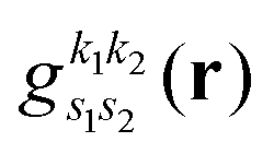 is the new Gaussian centered at
 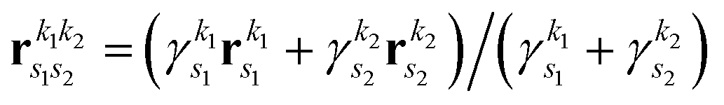 with exponent
 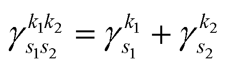 . Since the Cartesian coordinates (x,y,z) are linearly independent and each Gaussian function can be written as a product of x, y and z components,
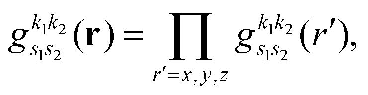
 . These can be determined analytically, as has been shown and tabulated in a previous publication.36


 different determinants.