Gradient-free determination of isoelectric points of proteins on chip

Abstract

The isoelectric point (pI) of a protein is a key characteristic that influences its overall electrostatic behaviour. The majority of conventional methods for the determination of the isoelectric point of a molecule rely on the use of spatial gradients in pH, although significant practical challenges are associated with such techniques, notably the difficulty in generating a stable and well controlled pH gradient. Here, we introduce a gradient-free approach, exploiting a microfluidic platform which allows us to perform rapid pH change on chip and probe the electrophoretic mobility of species in a controlled field. In particular, in this approach, the pH of the electrolyte solution is modulated in time rather than in space, as in the case for conventional determinations of the isoelectric point. To demonstrate the general approachability of this platform, we have measured the isoelectric points of representative set of seven proteins, bovine serum albumin, β-lactoglobulin, ribonuclease A, ovalbumin, human transferrin, ubiquitin and myoglobin in microlitre sample volumes. The ability to conduct measurements in free solution thus provides the basis for the rapid determination of isoelectric points of proteins under a wide variety of solution conditions and in small volumes.

---

1 Introduction

The isoelectric point (pI) is the value of the pH of a solution at which amphoteric molecules, such as proteins, have a vanishing net charge and hence no effective electrophoretic mobility.¹ Knowledge of the value of pI of a protein is particularly useful for separation² and purification,³ and for the characterisation of key physicochemical properties, such as surface charge and solubility, which are typically lower at values of the pH in the vicinity of the pI.⁴

A range of conventional methods can be used to determine the isoelectric point of proteins, including isoelectric precipitation,⁵ techniques based on ion-exchange adsorption,^6–8 zeta potential measurements,^9–11 capillary electrophoresis¹² or a recently developed nanoparticle-based approach.¹³ However, the predominant way to separate proteins and investigate their pI is isoelectric focusing (IEF), in which a pH gradient is generated across a chamber when an electric field is applied.¹⁴ Proteins that are then introduced into the system migrate in the gradient until they reach their pI and start to precipitate.¹⁵ A significant challenge underlying this approach is the requirement to generate and maintain a spatially stable pH gradient of a known and well controlled magnitude. One possible way to characterise such pH gradients is the use of a set of molecular markers, such as fluorescently labelled peptides or proteins, of known pI¹ to which the pI investigated sample can be added. This general principle of isoelectric focusing (IEF) can be applied using capillaries IEF,^1,16 gel slabs IEF¹⁷ or macro scale Free Flow Isoelectric Focusing (FFIEF).¹⁸

Microfluidic platforms are powerful technologies offering many advantages over bulk measurements, including high resolution, well controlled experimental conditions, low analyte volume requirement, short analysis time and low cost.^19–22 One currently used micro-scale approach for determining pI is microfluidic Free-Flow Isoelectric Focusing (μFFIEF),^23–25 which is based on the same principle as IEF with a pH gradient in the direction perpendicular to the advective flow in a microchannel.²⁶ The advantages offered by μFFIEF are rapid focusing of protein mixtures and protein complexes, accurate control of laminar flow and negligible Joule heating, although the quantitative control of maintenance and characteristic of spatial pH gradients remains a limitation.²⁷ IEF devices with spatial pH gradients have been created simply by mixing acidic and basic buffers, but this approach can be challenging to implement, because of difficulties in ensuring the stability of the gradient.²⁸ A significant improvement in this context is the invention of a “natural” pH gradient,²⁹ generated by the simultaneous use of several carrier ampholytes (CAs), amphoteric compounds with pI values close to each other. These compounds undergo a differential drift in an applied electric field and form a gradient,³⁰ that is nonlinear.³¹ Moreover, CAs and often markers can also interact with the protein under investigation and thus affect its pI.^16,31 Another potential drawback of CAs-gradients is the cathodic drift that can be due to the electromigration of CAs, electrolyte diffusion or electroosmosis,^30,32 and, moreover, the CAs approach is most reliable typically for samples under low salt concentration conditions.³² Despite the limitations of CAs, including their relatively high cost,³³ this μFFIEF gradient-model is constantly being improved^14,27 and is now commonly used for protein separation as well as the determination of pI values.

An alternative to the CAs approach is the use of an immobilized spatial pH gradient (IPG), in which monomeric buffering species are covalently linked to a polyacrylamide gel, this overcomes many of the drawbacks of the CAs approach, and many successful examples have been demonstrated.^32,34 This approach however, requires the casting of polyacrylamide gel with a spatial pH gradient, a process which can be challenging to automate and standarise to achieve a highly controlled linear gradient.³⁰ In addition to the gradient generated by carrier ampholytes or IPGs, there are less common CAs-free methods, such as thermally generated gradients,^33,35 electrolysis-induced pH gradients^36–38 and the promising technique of gradients created using diffusion potentials.³⁹

Although micron scale approaches for pI determination have great potential, and present many advantages over bulk techniques, the control of spatial pH gradients remains a challenge. To overcome this limitation, we introduce here a gradient-free method based on microfluidic Free-Flow Electrophoresis (μFFE) to determine the pI of a protein. We developed an approach that exploits temporal rather then spatial pH gradients in combination with μFFE as a tool to determine the isoelectric point of proteins. In this approach, the separation of a mixture of molecules is achieved by exploiting the difference in their charge-to-size ratios, which allows us to control the movement of molecules along the main advective direction of a separation chamber while applying an electric field perpendicularly to this direction. The positively charged molecules deflect towards the negative cathode, whereas negatively charged species migrate towards the positive anode.⁴⁰

In order to measure the deflection in the electric fields, the proteins studied here were initially labelled with ortho-pthalaldehyde (OPA) and imaged using an inverted fluorescence microscope. The analyte solution was introduced into the chip under native conditions (2 mM phosphate buffer pH 7.7) and the pH was only changed once the sample was within the microfluidic device (Fig. 1a); this process avoided the need to modulate the pH of the labelled protein off the chip prior its introduction to the device. To quantify accurately the electrophoretic mobility of the proteins under an applied electric field, we also monitored the DC current through the device, that together with the knowledge of the conductance of the buffer solution, allowed the magnitude of the electric field to be quantified.⁴¹ We then tested a series of buffers with different pH values to determine the pI from the dependence of the protein mobility on the pH, this approach has been extensively used in the macro scale.^12,42,43 We also investigated the influence of Tween-20, a biocompatible surfactant that aids in maintaining solubility of the protein samples close to their pI values, and also showed the effect of OPA labelling, on the isoelectric point value of proteins.

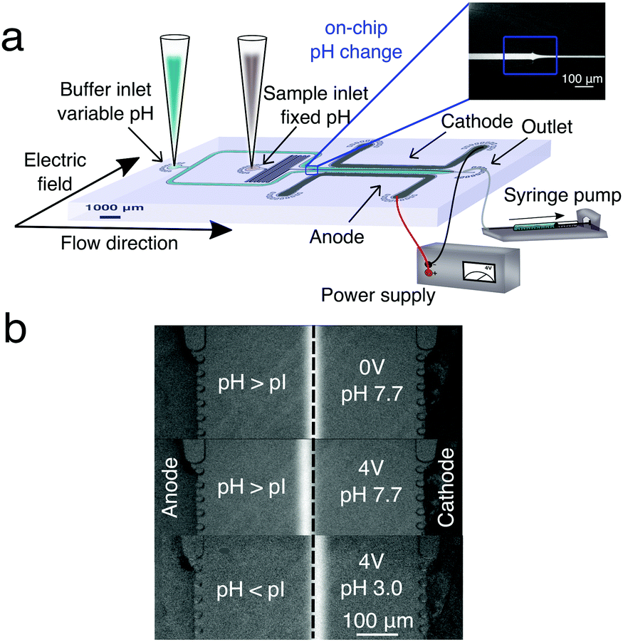Fig. 1 (a) Schematic diagram of the experimental setup for μFFE and gradient-free determination of protein isoelectric points. The microfluidic chip was designed such that a protein stream is flanked on either side by streams of buffer with variable pH. In the electrophoresis chamber (length = 5000 μm, height = 25 μm and width = 550 μm), the protein stream is deflected by a transverse electric field generated by lateral electrodes added in a single step during the PDMS chip fabrication.⁴¹ (b) Deflection of the BSA stream in a phosphate buffer at pH 7.7 > pI with no voltage applied (top), in a phosphate buffer at pH 7.7 > pI with 4 V applied (middle) and in a phosphate buffer at pH 3.0 < pI with 4 V applied (bottom).

2 Materials and methods

2.1 Preparation of protein samples and buffer systems

Bovine serum albumin (BSA), β-lactoglobulin (BLG), ribonuclease A (RNase A), ovalbumin (OVA), human serum transferrin (TF), ubiquitin (UB), myoglobin (MYO), ortho-pthalaldehyde, β-mercaptoethanol (BME), mono- and di-basic sodium phosphate, phosphoric acid, sodium hydroxide and the surfactant Tween-20 were obtained from Sigma-Aldrich (Gillingham, UK) and used without further purification.

A dye stock solution was prepared by dissolving OPA and BME in a ratio of 1 : 1.5 in 50 mM phosphate buffer at pH 8, to obtain final concentrations of 60 mM OPA and 90 mM BME. To prepare the analyte samples 2 mg of protein were dissolved in 990 μL of 2 mM phosphate buffer pH 7.7 (containing 0 v/v%, 0.01 v/v%, 0.1 v/v%, 1 v/v%, 2 v/v% of Tween-20) and then 10 μL of the dye stock solution were added, to give a final protein concentration of 2 mg mL⁻¹. In each case, the protein samples were freshly labelled prior to each experiment. For the rapid 2-point method no Tween-20 was added to the analyte samples, and no OPA was used for the label-free BSA* test. The 2 mM phosphate buffers solutions (pH 3, 3.3, 3.5, 3.8, 5.6, 6.6, 7.7, 8.0, 11.2) were prepared just prior to use by dilution of the 20 mM stocks, prepared in advance. The ionic strength for the 2 mM buffer solutions used during the experiment for pH range (3.0–7.7) was varied between 0.0017–0.0054 M. The pH was measured with the pH meter (Mettler Toledo MP 225, US).

2.2 Microfluidic device fabrication

A device master was first fabricated using standard UV lithography techniques. Briefly, a silicon wafer was spin coated with a 25 μm layer of negative photoresist SU8-3025 (Microchem, Massachusetts, USA) and baked on a hotplate at 98 °C for 12 min. Next, the wafer was exposed to UV light through the photomask (15 s, 16 mW) and post-baked at 98 °C for 5 min and unexposed photoresist was removed by developing with propylene glycol mono methyl ether acetate (PGMEA) Sigma-Aldrich (Gillingham, UK).

Devices for the measurements of pIs were replicated from the master using a mixture of 1 : 10 curing agent : polydimethylsiloxane elastomer (PDMS) (Sylgard 184, Dow Corning), degassed in a vacuum desiccator for 30 min and baked at 65 °C for 90 min. Each PDMS device was provided with fluidic access by punching inlets/outlet with a 0.75 mm biopsy puncher (Harris UniCore), washed with isopropanol (IPA) (Sigma Aldrich) and dried with nitrogen gas. The device was then chemically bonded to a microscope glass slide (Thermo Scientific) by activating both surfaces with an oxygen plasma (10 s, 40 mW) (Electronic Diener Femto Plasma Bonder) and baked at 65 °C for 10 min to improve adhesion. To prevent protein molecules sticking to the PDMS surface, a second plasma treatment (500 s, 80 mW) was applied to increase its hydrophylicity after bonding.⁴⁴

Electrodes were fabricated as reported previously.⁴¹ The microfluidic device was heated at 78 °C and alloy wires (51% In, 32.5% Bi, 16.5% Sn) (Indalloy, Conro Electronics) were inserted into the appropriate electrode inlets, and prevented from entering the main channel by carefully designed pillars. The diameter of the pillars was 25 μm and the distance between them was also 25 μm. As a next step the main channel of each device was quickly filled with water to maintain the surface hydrophilicity. Finally, copper wires were soldered to the alloy electrodes and connected to an external power supply.

2.3 Gradient-free microfluidic free-flow electrophoresis (μFFE)

The conditions and statistical analysis used for both 6-point and rapid 2-point methods are described below. Using a 1 mL glass syringe (Hamilton) with a 0.5 × 16 mm needle (Neolus Terumo) and 0.38 mm inner diameter tubing (Smiths Medical) the main channel of each device was filled manually from the outlet with 2 mM phosphate buffer at the desired pH value. The same buffer and the analyte were introduced via gel loading pipette tips into the inlets (Fig. 1a).

The total fluid flow (250 μL h⁻¹) through the devices was controlled by applying a reduced pressure via a neMESYS syringe pump (Cetoni) at the outlets, and the electrodes were connected to a power supply via copper wires. After 8 min of equilibration at the standard flow-rate the intensity of the protein beam was constant and deflection measurements were acquired. A range of electric potentials was applied across the device in 0.5 V steps up to a maximum of 4 V. For each voltage interval, three snapshots of the deflected protein beam were taken (at the end of the main channel) and three measurements of the electrical current were made using a digital multimeter. An inverted microscope (Zeiss AxioObserver, Germany) equipped with a UV LED, a filter Chromo 49000 DAPI and a 10× objective was used for all the optical measurements. For label-free measurements, which relied on the intrinsic fluorescence of aromatic amino acids, a custom-built deep UV-fluorescence microscope was used. Pictures of the deflected protein beam were acquired with a camera (Evolve 512) at an exposure time of 500 ms, and the same procedure was repeated for phosphate buffers with different pH values. For each pH value used the deflection measurement was repeated four times in 4 min intervals. To change the buffer the main channel was washed through the outlet with 200 μL of Milli-Q water using the tubing and a 1 mL Norm-Ject (Fisher Scientific) plastic syringe to avoid a significal increase in pressure which can damage the electrodes.

To quantify the deflection of the beam of the protein solution, the optical images acquired were analysed with ImageJ and custom software written in Python. After a series of the deflection measurements for all buffers were recorded with the different pH values, the device cell constant was calibrated for a KCl conductivity standard (Sigma-Aldrich) of 500 μS cm⁻¹ and for all tested buffers.⁴¹ Using a conductivity standard and the calculated conductance G, the cell constant K for each device was obtained as K = σ/G. The average cell constant of all the data presented in this paper was (49.6 ± 3.2 cm⁻¹). Recording the current, I, during the deflection measurements and from the conductance value obtained for the specific buffers, the effective voltage was calculated from V_e = I/G. Knowing V_e and the distance between the electrodes (w = 600 μm) allowed the electric field, E = V_e/w, to be calculated. The electrophoretic velocity v was determined by dividing the deflection δ by the residence time t, v = δ/t. In low aspect ratio channels the residence time at the centre of the channel can be approximated as the ratio of the device volume to the flow rate. Finally, to obtain the electrophoretic mobility μ, the migration velocity was divided by the electric field μ = v/E.

2.4 Quantitative labelling analysis

The proteins were labelled with a fluorogenic dye which reacts with protein primary amine groups (lysine residues, and the N-terminus).⁴⁵ To determine the extent of modification with OPA, and any effect that this may have on the protein pI, we compared the fluorescence intensity for proteins labelled under our conditions (pre-labelled) to model substrates (BSA, BLG, UB and the amino acid lysine (Sigma-Aldricht)), which were labelled under the conditions we had previously shown permitted quantitative modification of all reactive groups, and thus determination of protein concentration from the fluorescence intensity.⁴⁶ The labelling solution was prepared by mixing 16 mg (12 mM) of OPA with 4 mL of 500 mM carbonate buffer pH 10.5 and 4 mL of water. As a next step 12.3 μL (18 mM) BME and 2 mL of 20 w/v% of the anionic surfactant sodium dodecyl sulphate (SDS) (Sigma-Aldrich) were then added to the solution. The vial containing the solution of the labelling cocktail was then wrapped in aluminium foil, left in the oven for 15 min at 65 °C, and filtered using Millex-GP 0.22 μm filter (Merck Millipore).

Serial dilutions of BSA, BLG, UB, and lysine varying in concentration between 30 μM and 1.8 nM were prepared in 2 mM phosphate buffer solution at pH 8. Then, 2 mg mL⁻¹ of OPA-pre-labelled BSA, BLG and UB samples were prepared and diluted to 0.3 μM, and all the samples, and a background solution consisting of buffer and OPA, were placed in the wells of a half-area non-protein binding microplate (#3881, Corning) in triplicate. Using a CLARIOstar microplate reader (BMG LabTech), 50 μL of labelling cocktail was injected (430 μL s⁻¹) into each well containing 50 μL of unlabelled BSA, BLG, UB and lysine solutions to quantitatively label the samples, and the fluorescence intensity of each sample measured 3 s after dye injection. The fluorescence intensities of the pre-labelled BSA, BLG and UB solutions, corresponding to the “partially labelled” conditions used in this paper, were also measured, and the measurement for BSA repeated after 2 h (the maximum amount of time which passed during sample preparation and measurement for the experiments reported in this paper). The results were analysed using a custom Matlab program.

3 Results and discussion

3.1 Determination of the isoelectric point of BSA

BSA is a well characterized protein commonly used as a biophysical model system; we first set out to determine its isoelectric point using our gradient free μFFE approach. To do this, we recorded the deflection of streams of analyte co-flowing between streams of buffer of varying pH. The measurements were made using 2 mM phosphate buffers with different pH values (pH 3, 3.3, 3.8, 5.6, 6.6, 7.7). When the DC voltage (at 0.5 V intervals from 0 V to 4 V) was applied across the buffers with pH values higher than the pI of protein, the BSA molecules were negatively charged, and observed to move towards the anode (Fig. 1b, top, middle). In contrast, when buffers with pH values lower than the protein pI were used, the BSA molecules were positively charged and moved towards the cathode (Fig. 1b, bottom).

The deflection was measured four times in each device for each pH value, and was found to increase monotonously for enhancing voltages (Fig. 2a). When the maximum voltage (4 V) used in this study was reached, the highest average deflection (−17.8 ± 1.7 μm) was observed for solutions pH 7.7, while a lower average value (12.4 ± 2.3 μm) was observed for a solution with pH 3.0, which is closer to the pI for BSA. Moreover, deflection data for pH 7.7 were more reproducible than for pH 3. This fact can be explained by observing that BSA was always labelled with OPA off-chip in a buffer at pH 7.7. Hence during on-chip measurements at low pH (3, 3.3, 3.8) the buffer transitioned from pH 7.7 to lower pH at the nozzle, promoting BSA precipitation at pH = pI and the formation of a deposit, which has the propensity to affect the uniformity of the protein beam in the main channel. We explored two different paths (in this section, and in Section 3.2) to address this limiting factor both by modulating the flow rates and through the presence of a bio-compatible surfactant.

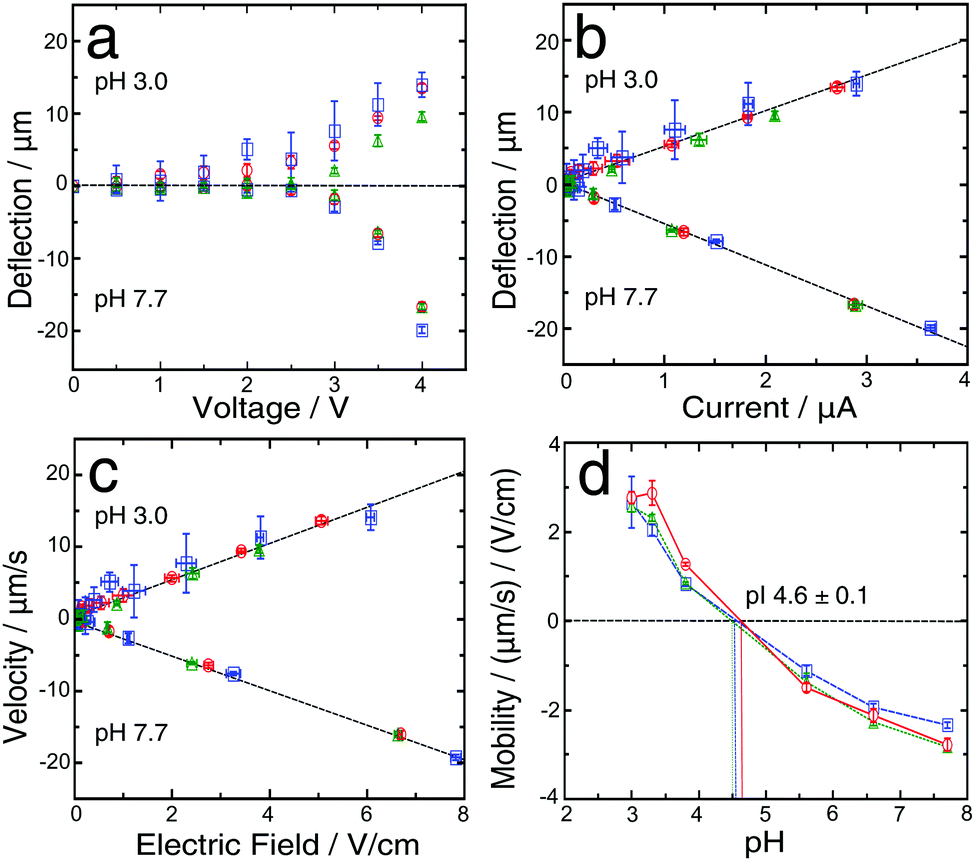Fig. 2 (a) Dependence of the analyte beam deflection as a function of the applied voltage for three different devices at pH 3.0 and 7.7. The stream deflection was measured at the end of the 5 mm long device channel, the maximal applied voltage was 4 V and was increased in steps of 0.5 V. (b) Dependence of the stream deflection on the current measured for the same data sets as in (a). (c) Dependence of the protein velocity on the applied electric field for the same data sets as in (a). (d) Dependence of mobility on pH for the same data sets as in (a). The intersections between the plots and the black dashed line (μ = 0) indicate the isoelectric point of BSA. The points and error bars indicate the mean and standard deviation obtained by averaging the mobility values of four different measurements per device for each pH analysed.

The flow rate during the deflection measurements was typically maintained at 250 μL h⁻¹; however, to avoid precipitation at the nozzle, for the low pH solutions, a higher flow rate (500 μL h⁻¹) was applied for the first 4 min of the equilibration step and afterwards decreased to 250 μL h⁻¹ and this procedure led to accurate measurements of the deflection. The beam deflection was found to correlate linearly with the simultaneously measured current⁴¹ (Fig. 2b); similarly, the electrophoretic velocity correlates linearly with the electric field (Fig. 2c) for pH 3.0 and 7.7 solutions and for all the other investigated pH values.

In order to estimate the protein isoelectric point several methods have been previously reported.^{12,42,43,47–49} Here we used linear interpolation. By using this approach, only the two points closest to the pI play a crucial role in analysing its value, although for a protein with unknown pI it is necessary to test a range of pH values. In our case values for the isoelectric point of BSA have been reported, so appropriate buffers were chosen accordingly. The pI obtained, in this way, which was based on the average for three devices, was 4.6 ± 0.1, and was the intersection of the curve and the μ = 0 line (Fig. 2d). This result is consistent with the values previously reported in the literature (4.5–5.1).^50–53 This confirms that our technique provides an accurate measurement of the protein's pI.

3.2 pI measurements in the presence of a bio-compatible surfactant

To enhance the solubility of proteins close to their pI value and eliminate adhesion problems at pH values close to the pI (Fig. 3a–c), we explored the addition of a Tween-20 surfactant to the BSA solutions during the labelling reaction at four different concentrations, 0.01, 0.1, 1 and 2 v/v% (Fig. 3e–h). This non-ionic and non-toxic surfactant is highly biocompatible, preserves the native protein structure,^54–56 increases protein solubility and reduces protein adsorption on the device surfaces.^57,58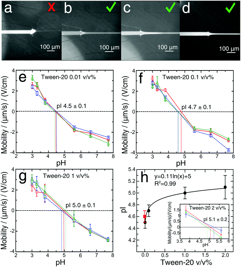

Fig. 3 (a) The nozzle of the microfluidic device was blocked by the precipitation of BSA at pH 3.0 and at a flow rate of 250 μL h⁻¹. (b) Formation of a BSA deposit close to the nozzle at pH 3.0 and an initial flow rate 500 μL h⁻¹ 2 min after the start of the measurement. (c) Formation of a BSA deposit under the same conditions as in (b), but after 4 min from the start of the measurement. The flow rate was then reduced to 250 μL h⁻¹ and the system was equilibrated for 4 min to allow accurate measurement of the beam deflection. In (a–c) Tween-20 was not added. (d) The stream of BSA flowing through the microfluidic nozzle at a flow rate of 250 μL h⁻¹, but with the addition of 0.1 v/v% of Tween-20 to the solution. The mobility as a function of pH for three different devices for (e) 0.01 v/v%, (f) 0.1 v/v%, (g) 1 v/v% of Tween-20 added to the protein solution during the preparation. The data points and error bars show the mean and standard deviations obtained by averaging four different measurements of the mobilities obtained for each pH and device. (h) Dependence of pI on Tween-20 concentration (v/v%). The data points and error bars show the mean and standard deviations obtained by averaging the pIs measurements obtained for three devices. The red square represents the mean of measurements performed without surfactant addition. The black line is a logarithmic fitting to the data. The inset presents the mobility as a function of pH for three different devices, measured at pH 3.8 and 5.6 and with 2 v/v% of Tween-20 addition to the protein solution.

It is commonly assumed that the presence of Tween-20 does not affect the pIs of proteins.⁵⁷ Here, with the microfluidic measurement device, we set out to test this hypothesis. Addition of 0.01 v/v% Tween-20 to the BSA solution (Fig. 3e) resulted in a pI value (4.5 ± 0.1), that was essentially identical to that determined for the measurement without Tween-20 (Fig. 2d). Nevertheless, this amount of Tween-20 was not sufficient to avoid the formation of any deposits in the solution. The concentration of the surfactant was increased to 0.1 v/v%, a value commonly used in the literature,^23,26,27 and with this amount of Tween-20, we did not observe the formation of any deposits of protein at any pH value (Fig. 3d). We measured an isoelectric point of 4.7 ± 0.1 (Fig. 3f) in accordance with the value obtained without the surfactant. This demonstrates that 0.1 v/v% Tween-20 concentration does not affect the protein pI measurement while avoiding the formation of protein deposit. At the concentration of Tween-20 of 1 v/v% (Fig. 3g) and 2 v/v% (Fig. 3h, inset) the pI changed significantly (5.0 ± 0.1) and (5.1 ± 0.2) respectively in comparison to the one obtained without the surfactant (Fig. 2d). The results, as shown in Fig. 3h, indicate that by increasing the amount of the surfactant Tween-20 in the analyte solution, a slow increase in pI was observed. These data indicate, therefore that the higher concentration of Tween-20 may affect the pI of protein. A possible reason behind this observation could be related to the critical micelle concentration of Tween-20 (CMC = 0.007–0.05 v/v%)^55,56 above which surfactant micelles formed,⁵⁹ and thus non-ionic micelles interact hydrophobically with protein ions in the applied electric field can induce changes in the electrophoretic mobilities^57,60 or modulate the deprotonation free energies of acidic residues.

3.3 Influence of labelling on pI determination

To permit visualisation with a standard epifluorescence optical microscopy setup, we labelled BSA with a fluorogenic dye, ortho-pthalaldehyde, which becomes fluorescent on reaction with primary amine groups exposed on the protein surface, such as lysine residues. However, this procedure removes positive charges below the pK_a of lysine (10.5 ± 1.1⁶¹). Therefore, at pH values below the pK_a of lysine, the protein is more negatively charged, and the value of the pI can be lowered.

We first determined the number of lysine residues that have reacted with the OPA, under the conditions used in this study. To obtain this information, we compared the fluorescence intensity measured for BSA which had been pre-labelled with OPA using our method, versus using another method⁴⁶ where lysine residues are quantitatively labelled with OPA as described in the Methods section. From the point (Fig. 4, intersection of the black/grey dashed lines) for quantitatively labelled BSA at 0.3 μM, we know the fluorescence intensity when all lysines react with the dye. The fluorescence intensity of pre-labelled BSA (Fig. 4, dark blue diamond) allowed us to calculate the percentage of lysines which reacted with OPA during our experiment. We showed that only 9 Lys (15%) reacted with OPA. We also showed that the number of labelled Lys did not increase with the time of experiment (Fig. 4, light blue diamond), but even slightly decreased, due to the instability of the isoindole fluorophore formed in this reaction.⁴⁶ Additionally to confirm those data we repeated the experiment for BLG and UB, which had similar labelling efficiencies, at 10.5% and 10.6% primary amines respectively. It can thus be suggested that in our electrophoretic experiments, OPA labelling does not affect significantly the values of isoelectric points for proteins.

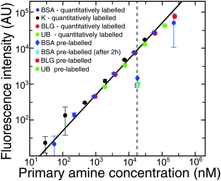Fig. 4 Dependence of the fluorescence intensity of BSA (dark blue circles), lysine (black circles), BLG (red circles) and UB (green circles) 3 s after mixing with the labelling solution on the concentration of reactive groups, primary amines. The intersection of the fitting (black line) and dashed grey lines shows quantitatively labelled BSA, BLG and UB at 0.3 μM. The dark blue diamond is the value of 0.3 μM pre-labelled BSA (5 min before measurement), while the light blue one is 0.3 μM pre-labelled BSA obtained 2 h after the first measurement. The red/green squares are values of 0.3 μM pre-labelled BLG and UB respectively. The data points and error bars show the mean and standard deviations obtained by averaging triplicates of the fluorescence intensity measurements.

3.4 Rapid two-point pI measurement

We have next developed a procedure for the rapid estimation of the pI values of proteins without a full titration curve using the microfluidic platform, which could be a useful tool for separation or purification processes. By analysing literature data⁶² containing a variety of pIs of proteins, approximately 70% have a pI between 4 and 7; by measuring the deflections at two values of pH, one below and one above this range we can estimate the unknown pI of protein. The deflection measurements were made using 2 mM phosphate buffers with pH values (3.0 and 7.7) for BLG and (3.3 and 7.7) for all other proteins. By calculating the mean and standard error of three independent measurements we obtained a BSA pI of 5.1 ± 0.2 (Fig. 5a, dark blue). The value was slightly higher than the one determined by using six different buffer pH values (4.6 ± 0.1), however, it was in accordance with the values previously reported in the literature (4.5–5.1).^50–53 In the two-point procedure only the extreme two values (Fig. 2d) were considered in the calculation, so that the calculated pI was shifted towards higher values. Moreover, this method was also used to provide further confirmation of the minimal effect of protein labelling under our conditions on the measured protein pI. The same two-point μFFE experiment was performed in a label-free manner using a deep UV fluorescence setup. The pI value for label-free BSA* was 5.0 ± 0.2 (Fig. 5a, light blue), indistinguishable within error to the two-point measurement for labelled BSA. All the conditions and the statistical analysis for OPA-labeled and label-free approaches were described previously in Section 2.3.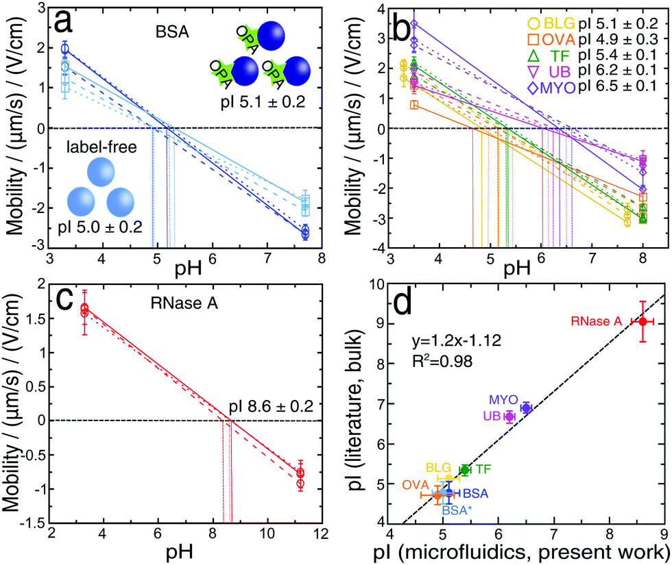

Fig. 5 Dependence of the electrophoretic mobility on pH for (a) bovine serum albumin, (b) β-lactoglobulin, ovalbumin, human transferrin, ubiquitin, myoglobin, (c) ribonuclease A; without the addition of the Tween-20 surfactant. (a) The measurements were performed for OPA-labelled BSA (dark blue) and unlabelled BSA* (light blue). The intersections between the plots and the black dashed line (μ = 0) indicate the isoelectric points of proteins. The data points and error bars show the mean and standard deviation obtained by averaging the mobility values of four different measurements per device for each pH analysed. (d) Comparison of experimental and literature pI values. The x values are the mean and standard deviation obtained by averaging three pI measurements per protein, by using our rapid 2-point approach. The y values indicate the mean and standard deviation of four (BSA, BSA*) and three (BLG, TF, UB, RNase A) single values of pI from the literature. For OVA and MYO the range presented in the literature was also averaged and standard deviation obtained.

We further explored the generality of this approach by measuring the pIs of β-lactoglobulin, ovalbumin, transferrin, ubiquitin and myoglobin (Fig. 5b). We also examined ribonuclease A, as an example of the protein which is outside the pH range (4–7) (Fig. 5c); by increasing the higher value of pH to 11.2. The obtained result (8.6 ± 0.2) was in accordance with previously reported values (8.6–9.6).^53,63,64 Similarly, the values measured for other proteins were in accordance with literature values: BLG 5.1 ± 0.2 (5.1–5.2),^7,65,66 OVA 4.9 ± 0.3 (4.6–4.9),⁶⁷ TF 5.4 ± 0.1 (5.2–5.5),^68,69 UB 6.2 ± 0.1 (6.5–6.8)^70–72 and MYO 6.5 ± 0.1 (6.8–7.0).⁷³ By plotting the dependence of the literature and the experimental values of pIs (Fig. 5d), we observed a linear correlation with the high coefficient of R² = 0.98.

4 Conclusions

In this paper, we have reported a microfluidic device based on μFFE for the determination of protein isoelectric points, by varying the pH in time, rather than in space, allowing for reproducible measurement of pIs without the requirement for the generation of a pH gradient, which is often challenging in practice (μFFIEF). Using this approach we have obtained pIs for BSA, which are identical within experimental error with the values reported in the literature. The method also requires low voltages, and low sample consumption, and devices can be fabricated using inexpensive consumables. We also showed that it is possible to estimate pI values for a wide range of proteins (BLG, RNase A, OVA, TF, UB, MYO) from electrophoretic mobilities in free solution, measured at only two pH values. These results suggest that gradient-free determination of isoelectric points is rapid and accurate measurement of pI value on small volume of samples.

Acknowledgements

We acknowledge financial support from the Biotechnology and Biological Sciences Research Council, the Newman Foundation and the Elan Pharmaceuticals. The research leading to these results has also received funding from the European Research Council under the European Union's Seventh Framework Programme (FP7/2007-2013) through the ERC grant PhysProt (agreement n° 337969).

References

1. P. Righetti, J. Chromatogr. A, 2004, 1037, 491–499.
2. B. Walowski, W. Huttner and H. Wackerbarth, Anal. Bioanal. Chem., 2011, 401, 2465–2471.
3. W. Goldman and J. Baptist, J. Chromatogr., 1979, 179, 330–332.
4. R. K. Scopes, Protein Purification Principles and Practice, Springer, Bundoora, Australia, 2nd edn, 1987.
5. W. Jaffe, J. Biol. Chem., 1943, 148, 185–186.
6. V. C. Yang and R. S. Langer, US Pat., 4666855 A, 1987.
7. S. Yamamoto and T. Ishihara, J. Chromatogr. A, 1999, 852, 31–36.
8. Y. Sakakibara and H. Yanagisawa, Bull. Aichi Univ. Educ., 2007, 56, 45–49.
9. P. S. Santiago, F. A. O. Carvalho, M. M. Domingues, J. W. P. Carvalho, N. C. Santos and M. Tabak, Langmuir, 2010, 26, 9794–9801.
10. J. Y. Jun, H. H. Nguyen, S.-Y.-R. Paik, H. S. Chun, B.-C. Kang and S. Ko, Food Chem., 2011, 127, 1892–1898.
11. S. Salgin, U. Salgin and S. Bahadir, Int. J. Electrochem. Sci., 2012, 7, 12404–12414.
12. Y. Yao, K. Khoo, M. Chung and S. Li, J. Chromatogr. A, 1994, 680, 431–435.
13. S. Pihlasalo, L. Auranen, P. Hanninen and H. Harma, Anal. Chem., 2012, 84, 8253–8258.
14. C. Herzog, E. Beckert and S. Nagl, Anal. Chem., 2014, 86, 9533–9539.
15. M. Roman and P. Brown, Anal. Chem., 1994, 66, A86–A94.
16. J. Wu and T. Huang, Electrophoresis, 2006, 27, 3584–3590.
17. B. Cargile, J. Bundy, T. Freeman and J. Stephenson, J. Proteome Res., 2004, 3, 112–119.
18. M. Islinger and G. Weber, Methods Mol. Biol., 2008, 432, 199–215.
19. G. M. Whitesides, Nature, 2006, 442, 368–373.
20. T. P. Burg, Microsystems for pharmatechnology: manipulation of fluids, particles, droplets, and cells, Springer, Switzerland, 1st edn, 2016.
21. V. Busin, B. Wells, M. Kersaudy-Kerhoas, W. Shu and S. T. G. Burgess, Mol. Cell. Probes, 2016, 30, 331–341.
22. N. P. Beard, J. B. Edel and A. J. deMello, Electrophoresis, 2004, 25, 2363–2373.
23. Y. Xu, C. Zhang, D. Janasek and A. Manz, Lab Chip, 2003, 3, 224–227.
24. K. S. Yang, P. Clementz, T. J. Park, S. J. Lee, J. P. Park, D. H. Kim and S. Y. Lee, Curr. Appl. Phys., 2009, 9, E66–E70.
25. J. Wen, E. W. Wilker, M. B. Yaffe and K. F. Jensen, Anal. Chem., 2010, 82, 1253–1260.
26. D. Kohlheyer, G. Besselink, S. Schlautmann and R. Schasfoort, Lab Chip, 2006, 6, 374–380.
27. D. Kohlheyer, J. C. T. Eijkel, S. Schlautmann, A. van den Berg and R. B. M. Schasfoort, Anal. Chem., 2007, 79, 8190–8198.
28. A. Kolin, J. Chem. Phys., 1954, 22, 1628.
29. H. Svensson, Acta Chem. Scand., 1961, 15, 325–341.
30. G. J. Sommer and A. V. Hatch, Electrophoresis, 2009, 30, 742–757.
31. G. J. Sommer, A. K. Singh and A. V. Hatch, Anal. Chem., 2008, 80, 3327–3333.
32. B. Bjellqvist, K. Ek, P. Righetti, E. Gianazza, A. Gorg, R. Westermeier and W. Postel, J. Biochem. Biophys. Methods, 1982, 6, 317–339.
33. T. Huang and J. Pawliszyn, Electrophoresis, 2002, 23, 3504–3510.
34. J. W. Albrecht and K. F. Jensen, Electrophoresis, 2006, 27, 4960–4969.
35. M. Becker, A. Mansouri, C. Beilein and D. Janasek, Electrophoresis, 2009, 30, 4206–4212.
36. K. Macounova, C. Cabrera, M. Holl and P. Yager, Anal. Chem., 2000, 72, 3745–3751.
37. K. Macounova, C. Cabrera and P. Yager, Anal. Chem., 2001, 73, 1627–1633.
38. C. Cabrera, B. Finlayson and P. Yager, Anal. Chem., 2001, 73, 658–666.
39. Y. Song, S. Hsu, A. Stevens and J. Han, Anal. Chem., 2006, 78, 3528–3536.
40. N. Pamme, Lab Chip, 2007, 7, 1644–1659.
41. T. W. Herling, T. Mueller, L. Rajah, J. N. Skepper, M. Vendruscolo and T. P. J. Knowles, Appl. Phys. Lett., 2013, 102, 184102.
42. N. Ui, Biochim. Biophys. Acta, 1972, 257, 350–364.
43. N. Douglas, A. Humffray, H. Pratt and G. Stevens, Chem. Eng. Sci., 1995, 50, 743–754.
44. S. H. Tan, N.-T. Nguyen, Y. C. Chua and T. G. Kang, Biomicrofluidics, 2010, 4, 032204.
45. M. Roth, Anal. Chem., 1971, 43, 880–882.
46. E. V. Yates, T. Mueller, L. Rajah, E. J. De Genst, P. Arosio, S. Linse, M. Vendruscolo, C. M. Dobson and T. P. J. Knowles, Nat. Chem., 2015, 7, 802–809.
47. P. Tartaj, O. Bomati-Miguel, A. F. Rebolledo and T. Valdes-Solis, J. Mater. Chem., 2007, 17, 1958–1963.
48. J. Floury, I. El Mourdi, J. V. C. Silva, S. Lortal, A. Thierry and S. Jeanson, Front. Microbiol., 2015, 6, 1–12.
49. S. Ross and R. Ebert, J. Clin. Invest., 1959, 38, 155–160.
50. H. Gao, C. Li, F. Ma, K. Wang, J. Xu, H. Chen and X. Xia, Phys. Chem. Chem. Phys., 2012, 14, 9460–9467.
51. C. Chaiyasut, Y. Takatsu, S. Kitagawa and T. Tsuda, Electrophoresis, 2001, 22, 1267–1272.
52. A. Conway Jacobs and L. Lewin, Anal. Biochem., 1971, 43, 394–400.
53. T. J. Bruno and P. D. N. Svoronos, Handbook of basic tables for chemical analysis, CRC Press, 2nd edn, 2004.
54. A. Mulchandani, W. S. Adney, J. D. McMillan, J. R. Mielenz and T. K. Klasson, Applied Biochemistry and Biotechnology, Biotechnology for Fuels and Chemicals: The Twenty-Ninth Symposium, Humana Press, USA, 2010.
55. B. A. Kerwin, J. Pharm. Sci., 2008, 97, 2924–2935.
56. T. Imae, Advanced Chemistry of Monolayers at Interfaces, Trends in Methodology and Technology, Academic Press, The Netherlands, 1st edn, 2007.
57. A. Malhotra and J. Coupland, Food Hydrocolloids, 2004, 18, 101–108.
58. M. Feng, A. Morales, A. Poot, T. Beugeling and A. Bantjes, J. Biomater. Sci., Polym. Ed., 1995, 7, 415–424.
59. C. Holtze, A. C. Rowat, J. J. Agresti, J. B. Hutchison, F. E. Angile, C. H. J. Schmitz, S. Koster, H. Duan, K. J. Humphry, R. A. Scanga, J. S. Johnson, D. Pisignano and D. A. Weitz, Lab Chip, 2008, 8, 1632–1639.
60. T. Takayanagi and S. Motomizu, J. Chromatogr. A, 1999, 853, 55–61.
61. G. R. Grimsley, J. M. Scholtz and C. N. Pace, Protein Sci., 2009, 18, 247–251.
62. D. Malamud and J. Drysdale, Anal. Biochem., 1978, 86, 620–647.
63. S. Dubey and Y. N. Kalia, J. Controlled Release, 2010, 145, 203–209.
64. Y. Li, H. Yang, Q. You, Z. Zhuang and X. Wang, Anal. Chem., 2006, 317–320.
65. Y. Guo, P. Harris, L. Pastrana and P. Jauregi, Food Hydrocolloids, 2017 DOI:10.1016/j.foodhyd.2017.04.027.
66. P. Majhi, R. Ganta, E. Vanam, K. Giger and P. Dubin, Langmuir, 2006, 22, 9150–9159.
67. E. Smith, J. Biol. Chem., 1935, 108, 187–194.
68. P. Albertsson, S. Sasakawa and H. Walter, Nature, 1970, 228, 1329–1330.
69. Y. Gao, C. Chen, Z. Chai, J. Zhao, J. Liu, P. Zhang and Y. Huang, Analyst, 2002, 1700–1704.
70. J. Durner and P. Boger, J. Biol. Chem., 1995, 270, 3720–3725.
71. K. Wilkinson and T. Audhya, J. Biol. Chem., 1981, 9235–9241.
72. S. Koenig, D. Ackermann, W. Weiqun and L. Gruen, EP2715331 A1, 2014.
73. J. Chmelik and W. Thormann, J. Chromatogr., 1992, 600, 305–311.

---