Probing the average distribution of water in organic hydrate crystal structures with radial distribution functions (RDFs)

Abstract

The abundance of crystal structures of solvated organic molecules reflects the common role of solvent in the crystallisation process. An understanding of solvation is therefore important for crystal engineering, with solvent choice often affecting polymorphism as well as influencing the crystal structure. Of particular importance is the role of water, and a number of approaches have previously been considered in the analysis of large datasets of organic hydrates. In this work we attempt to develop a method suitable for application to organic hydrate crystal structures, in order to better understand the distribution of water molecules in such systems. We present a model aimed at combining the distribution functions of multiple atom pairs from a number of crystal structures. From this, we can comment qualitatively on the average distribution of water in organic hydrates.

---

Introduction

The crystallisation of organic hydrates commonly occurs in the isolation of active materials in the pharmaceutical and specialist chemical industries.¹ This is reflected in the abundance of such structures; for example the Cambridge Structural Database (CSD) was reported to include around 70 000 structures of organic and organometallic systems found to contain water in some form^2,3 (2010).

The abundance of hydrates reflects the common role of solvent in the crystallisation process. An understanding of this is therefore of paramount importance for crystal engineering, with solvent choice often influencing the crystal structure and properties; either by formation of a solvate or hydrate, by directing the molecular conformation, or by favouring a particular crystal packing.

The systematic analysis of hydrates was, until recently, often confined to inorganic structures.⁴ Such investigations have been complemented by surveys of organic hydrates, which have served primarily as a tool for the classification of the role of water within the crystallisation process, and in overall structure. A commonly accepted classification system organises water sites within crystal structures into three main categories: isolated lattice sites, lattice channels and metal-ion coordinated water.⁵ Other survey studies have also considered the driving force for hydrate formation.^6–8

A recent discussion⁹ considers novel coordination environments, specifically in relation to hydrates. Emphasis is placed on the abundance of hydrates within crystal structures, implying that any discussion of hydrates should first consult the CSD. It is suggested that existing work directed toward characterisation of water motifs adequately describes the variety of possible motifs to an appropriate standard of notation.^10,11 This assumption is supported by the classification of apparently novel motifs by the authors' own classification system, and the classification of organic hydrates seems possible in the forms of either a three-category or a cluster-based approach. These methods of characterisation are commonly accepted and often cited within the literature.

van de Streek and Motherwell noted that “statistical surveys into the behaviour of hydrates are difficult due to the severe bias that is introduced at many levels⁸”, however there may be scope within similar surveying techniques for the building of predictive models. For example, Galek et al.¹² have utilised data available in the CSD to develop statistical models for hydrogen-bond coordination behaviour (not limited to the study of hydrates). Their work describes the hydrogen bonding behaviour of over 70 unique atom types, and begins to make assessments of structural stability of hydrogen bonding environments in known crystal structures, showing potential for application of empirically or statistically derived models.

In this work we develop a method for the statistical analysis of organic hydrate crystal structures.

Our model combines the radial distribution functions (RDFs) of multiple atom pairs from numerous organic hydrate crystal structures. We also compare water oxygen (OW) and water hydrogen (HW) RDFs to the work of Soper.¹³ Soper evaluated neutron diffraction data for water and ice at a range of temperatures (220 K to 673 K) and pressures (up to 400 MPa) in the form of OO, OH and HH partial structure factors. Fourier transformation of these partial structure factors produces site–site RDFs. However, the presence of systematic uncertainties arising from diffraction experiments means that this transformation is not as intuitively straightforward as expected. Soper uses empirical potential structure refinement (EPSR) in order to fit a 3D computational water model as closely as possible to the pre-determined experimental structure factors, improving the reliability of the extracted RDFs. Preliminary comparison of our own data with all of Soper's water and ice functions showed that our functions fit best (from visual overlay) with ice at 220 K, and water at 298 K, both under ambient pressure. Thus, comparisons between these two models and our own RDF will be discussed in depth.

Theory

RDFs are simply calculable from crystal structures by evaluating all interatomic distances of atom pairs, binning them into a histogram, and then normalising with respect to an unbiased distribution of the same number of atoms – hence accounting for the intrinsically increasing numbers of pairs at larger values of r. This is demonstrated for a heterogeneous system in the equation below;
where ρ_αβ represents the number density of pairs in the entire system volume, and n_αβ represents the number of pairs comprising atoms of species α and β. This function gives the probability of finding an atom of species β at a distance r from an atom of species α. The RDF for a particular material is often described graphically as a function of distance, r, with respect to the reference particle. The overall profiles of the plots of RDFs differ, depending on phase of matter, and the order present. For RDF plots of a crystal structure, g(r) is represented by a series of short spikes, which indicate the existence of particles at specific and definite locations. This regularity can be extended almost infinitely until the crystal edge, illustrating the long-range order that, at least ideally, symmetry imparts to crystal structures.

The profile of a liquid RDF differs greatly. The function represents an average of particle locations, conversely to the precise positions depicted in crystal structures. When a crystal melts to liquid, long-range order is lost, and at large distances there is an equal probability of finding a second particle in any shell of equal volume. However, at short distances close to the reference particle there may be some remaining order, a vestige of that found in the crystal phase. The nearest neighbours of the reference particle may still approximately occupy their original positions. Thus, it is often possible to identify an average sphere of nearest neighbours in the first and perhaps the second shell r₁ and r₂ from the reference particle.¹⁴

A useful description of the energetics of a solution can be extracted from the potential of mean force¹⁵ (PMF), which describes free energy changes of the system as a function of a coordinate or coordinates. A popular choice for the coordinate is the distance r, due to the simplicity of calculation.

For a given r between two molecules, the PMF describes an average over all orientations of the surrounding solvent molecules. RDFs are directly related to the PMF w²(r) by;

where (2) denotes the number of atoms or particles to be considered. Thus;

w⁽²⁾(r) = −kT ln g(r)

The Helmholtz free energy A(r) can be expressed as;

A(r) = −kT ln g(r) + a

where a is a constant chosen so that the most probable distribution between two particles gives a free energy of 0.

The PMF can be used to describe the energetics of the whole system. An appropriate weighting scheme applied to empirically parameterised RDFs can then be utilised within computational algorithms for the simulation of systems in solution. This reduces the computational cost associated with explicit solvent models, whilst improving some of the inaccuracies that implicit solvation models suffer due to their inherent approximations. A theoretical example of how RDFs and PMFs could be applied to predictive models in the future is given in the Future Application section below.

Methods

Calculation of radial distribution functions (RDFs)

In order to test the predictive power of a RDF model applied to non-crystalline phases, we included atom positions in a cumulative plot. We used the common atom-typing algorithm of the AMBER forcefield, and calculated RDFs for all atom types found within small-molecule organic hydrates.

The dataset for building of RDFs was obtained from a search for any structure containing water as an independent entity in the CSD (CSD version 5.34, 2013).¹⁶ Structures included in the dataset were selected with the following restrictions; 3D coordinates determined, R ≤ 0.05, not disordered, no errors, not polymeric, no powder structures, and only organic. All hydrogen positions were normalised according to the following criteria; C–H = 1.089 Å, N–H = 1.015 Å, O–H = 0.993 Å. The final dataset contained 5922 structures in total.

We developed a programmatic approach within MATLAB in order to automate the processing of the dataset, and to collate the results effectively for the building of RDFs.

The developed program's primary operation can be summarised as follows;

• Determine atom types according to AMBER forcefield definitions for a crystal structure .pdb file with Antechamber.^17,18

• Apply all crystallographic algorithms necessary to produce symmetry equivalent atom positions and to expand the lattice by one unit cell in each direction.

• Sort all atoms for each structure into individual arrays.

• Move the structure coordinate system origin to a target atom nucleus position (either water oxygen or hydrogen).

• Convert to a spherical polar coordinate system.

• Calculate distance, azimuth and elevation for all atom pairs within a specified cut-off distance (15 Å).

• Repeat, moving origin for every target atom in the system.

• Save data as a MATLAB workspace for manipulation with further routines.

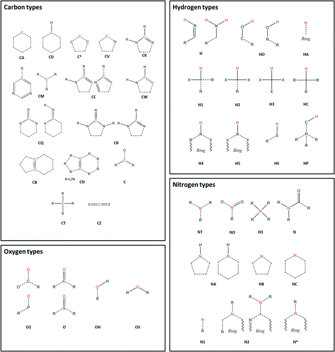
The libraries for all information relating to symmetry operations were developed from the existing Fortran library CrysFML,¹⁹ the Bilbao Crystallographic Server,^20–22 and the International Tables.²³ Routines for RDF calculations were developed from I.S.A.A.C.S²⁴ and from Allen and Tildesley.²⁵ Atom type assignment is performed as an external routine through Antechamber.^17,18 Schematic representations of the atom types used in this study are shown in Fig. 1.

Fig. 1 Schematic representations of AMBER atom types. The red colour represents the atom being typed. The code below each schematic refers to the code assigned by the AMBER routine. R groups represent any atom, and X groups represent either N or O. Dotted lines represent undefined bond order, and solid lines represent conventional nomenclature of bonds.

Deconvolution of water RDF by water motif

In order to break down the contribution of particular arrangements of water (within organic hydrate crystal structures) to the average distribution of HW⋯OW, as represented by our RDF, an investigation into the specific motifs present within our dataset was conducted.

The identification of motifs (as defined by Infantes and Motherwell¹⁰) was conducted using the CSD-Materials module, available in the current release of Mercury.²⁶ The selected motifs are represented in Fig. 2. The motifs can be separated into: infinite chains, discrete chains, discrete rings, and infinite tapes in one dimension.

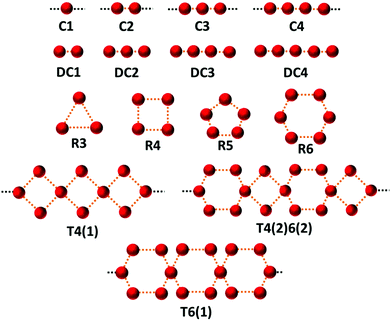Fig. 2 The 15 water motifs used in this work. The motifs can be separated into: infinite chains (C1, C2, C3, C4; the number represents the number of unique waters present before the motif is repeated), discrete chains (DC1, DC2, DC3, DC4; the number represents the number of contacts between waters in the chain), discrete rings (R3, R4, R5, R6; the number represents the number of waters in the ring), and infinite tapes in one dimension involving rings (T4(1), T4(2)6(2), T6(1); a number outside of brackets represents the number of waters in the ring motif, and a number inside of brackets represents the number of waters from this ring also involved in a neighbouring ring). Nomenclature taken, and figure adapted from Infantes and Motherwell.¹⁰

The search criteria for water motifs ignore specific hydrogen bonding interactions, and simply define a network by an O⋯O distance < sum vdW radii + 1 Å. Therefore, quantification of the intermolecular pair distances (HW⋯OW) is not directly possible from the search results themselves. In order to assess these interactions, the pair count histograms were selected from the original dataset, and a new RDF calculated for each motif.

Results

Structure of water in hydrates

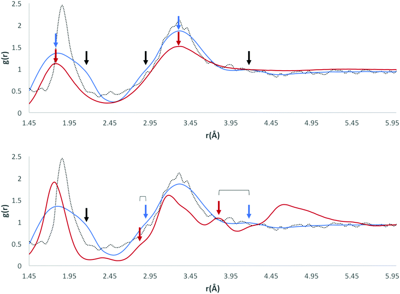
Our initial expectations were that only the direct intermolecular interactions (equivalent to the first solvation shell) would be deducible from the calculated RDFs, and that difficulties would arise in relating the distributions to the equivalent solution phase information. However, a comparison of our RDF for HW and OW with Soper's RDFs for ice (220 K; Fig. 3, bottom) and water (298 K; Fig. 3, top) and the calculated RDF of Bernal's hexagonal ice model,²⁷ does show some interesting correlations beyond the first solvation shell.

Fig. 3 A comparison of the short-range interactions in our RDF for OW⋯HW pairs (original data shown as dotted black lines, smoothed data shown in blue) with Soper's RDF of water at 298 K (shown in red on the top plot) and ice at 220 K (shown in red on the bottom plot). The black arrows on both plots represent peaks or features in our RDF which cannot be explained by the comparative Soper plot. The blue and red arrows indicate comparable peaks, with their colour corresponding to the same coloured plot line.

It is important to determine whether the discrete features observable in the RDF are in fact noise, or signal. There are two possible scenarios: A) the features present are noise, due to an insufficient amount of data, meaning the distribution is not entirely representative of a smooth and average distribution within hydrates; B) the features present are signal, comprising a number of discrete peaks occurring due to the complexity of the water networks or motifs found in organic hydrates.

Fig. 3 (bottom) shows Soper's EPSR model for ice at 220 K parameterised from neutron diffraction data (red), and our RDF (original: dotted black line, smoothed function: blue) resulting from all water oxygen to water hydrogen pair distances found within our dataset (5922 structures). It can be seen that there is a shift of the first two observable peaks to higher values of r, and the absence of the third peak observable in Soper's function. The peaks and troughs of the RDF profile also occur at different values of g(r). This difference is highly relevant if the model data from our RDF data are to be applied to predictive models in the future, particularly in the conversion of RDFs to PMFs, as the logarithmic relationship between g(r) and w(r) means that a small change in free energy (a small multiple of kT) can correspond to a change in g(r) of an order of magnitude from its expected or most likely value. However, one structural feature unique to the Soper ice RDF, which doesn't occur in the Soper water RDF, also appears to be present in our RDF; namely, the presence of a small peak in the trough between the two large peaks representing the first and second hydration shells, between 2–3 Å.

Overlaying the OW⋯HW RDF with Soper's model of water (298 K) provides a better fit in terms of peak positions, as shown in Fig. 3 (top; original: dotted black line, smoothed function: blue). However, discrete features unique to the solid state of ice are not present in Soper's liquid water function.

If the RDF model is compared to this subtle peak in Soper's water model, it can be seen that the maxima of the peaks in its profile, although quite noisy, fit the shape of the water profile well. No smoothing function has been applied as part our own method, however Soper fitted his data to inherently smooth computational models of water and ice.

A visual comparison of the short-range interactions discussed above is also summarised in Fig. 3. In both images, we have applied the Savitzky–Golay smoothing algorithm²⁸ to our data (shown as a blue line, with the original data as a black dotted line) simply for the purpose of producing this figure, in order to increase the signal-to-noise ratio without unduly distorting the original data. In the top image, we compare this to Soper's 298 K water model, and highlight three areas where our own RDF displays features that are not explained by the water model. Namely, a large shoulder on the right of the first interaction peak, at ∼2.15 Å, a smaller shoulder on the left of a second interaction peak, at ∼2.85 Å, and a third small but independent peak at ∼4.16 Å. We have also indicated peaks that are explained by the water RDF, as indicated by the blue and red arrows, highlighting the peaks in their respective plot colours.

In the bottom image, we compare our smoothed profile (blue) to Soper's ice RDF (red), and attempt to indicate sources for the unexplainable peaks from the ice profile, as indicated above. The first shoulder, indicated by the only black arrow in the bottom image, is not confidently explained by either of Soper's distributions, and is probably due to the broad distribution of data in the first solvation shell, and between the first solvation shell and the second solvation shell.

The overall shape of our profile correlates well to that of Soper's water profile. However, certain features present in Soper's ice RDF also appear in our RDF; i) a peak at 2.9 Å that becomes a shoulder on the peak at 3.3 Å when a smoothing algorithm is applied, corresponding to a similar feature of Soper's 220 K ice function, at 2.8 Å and ii) a peak at 4.1 Å, which is emphasised upon the application of a smoothing algorithm, corresponding to the third solvation shell, present in Soper's 220 K ice function at 3.8 Å. This suggests that some order found in a typical ice model is also present in the overall structure of water in organic hydrates. In liquid water, this order is lost, meaning that Soper's water model no longer contains these interactions. However, the peak positions in our RDF correspond more closely to those present in Soper's liquid water model than to the ice model.

The presence of peaks in similar positions to Soper's water function in our RDF may suggest that our data are most representative of systems at 298 K, implying that water networks within hydrates have similar interaction distances to liquid water. This may result from the measurement temperature of the original data; over half of the contributing structures (3659) were measured above 261 K. However, it could also be an indication of peak broadening in the RDF due to the diversity of structures within our dataset. Beyond the second solvation shell, the RDF appears to be noisy.

Additional consideration was given to the measurement temperature at which the crystallographic data were obtained. The data were separated into three 50 K temperature intervals, and one interval where the temperature was above 261 K. These intervals were chosen based upon the distribution of measurement temperatures across the whole dataset, with a large number of structures (over half of the dataset) being measured at ∼298 K. Next, the HW⋯OW RDFs were recalculated for each temperature interval. The resulting functions are shown in Fig. 4.

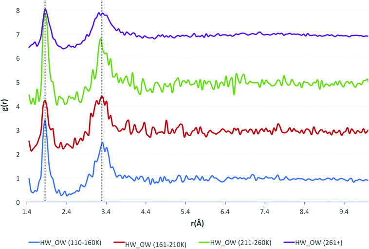Fig. 4 The HW⋯OW RDFs for water, separated by temperature ranges, as indicated by the legend (bottom) with the functions stacked in order of increasing temperature.

The positions of the peak maxima representative of the first and second solvation shells do not change, unlike the Soper functions. This is because of the normalisation of hydrogen bond lengths, done because hydrogen positions are notoriously difficult to assign in crystal structure solution and refinement. Unfortunately, this means that subtle differences in the data, reflecting the variation in lengths of covalent bonds to hydrogen, may occasionally be lost. However, it is unlikely that the data would be any more accurate or reliable should the hydrogen bond lengths not be normalised, and perhaps more errors would be incorporated into the data from unreliable bond lengths due to the unreliable assignment of hydrogen positions in the experimental data.

The only observable difference between the measurement temperature separated data are the values of g(r) at which the peak maxima occur, although there is no observable pattern to explain this. The number of contributing data were considered as a cause, but recalculating the functions with the same number of contributing structures for each temperature range produced similar results. The larger oscillations seen in the results at 211–260 K are due to there being fewer data in this range than in other intervals.

In order to determine whether discrete features at both short and long range were due to specific arrangements of water, further analyses of specific motifs were carried out.

We observe a better fit of the long-range pair distances to Soper's water model in comparison to the ice model. However, there is still a considerable amount of ‘noise’ present at long-range distances. This was investigated further by the overlay of the RDF with an RDF (calculated in I.S.A.A.C.S²⁴) for Bernal's hexagonal ice structure.²⁷ However, statistical analysis of the long range pair distances (>4 Å) for both of the Soper functions and also for the hexagonal ice function (Table 1) showed that the profile of water (298 K) fits best, followed by ice (220 K) and finally hexagonal ice.

Table 1 A summary of the statistical analysis of GOF for the long range pair distances of the HW⋯OW RDF with hexagonal ice, water (298 K) and ice (220 K) models

	Hexagonal ice	Water (298 K)	Ice (220 K)
RMSE	8.7	0.57	0.62
ln(L)	−640	−154	−170
AIC	1287	314	345
BIC	1297	324	355

---

Log of Likelihood (ln(L)), the Akaike information criterion (AIC), and the Bayesian information criterion (BIC) were used as statistical measures for goodness of fit (GOF). The AIC is a measure that aims to select the best approximating model from a group of non-linear models.²⁹ Given a collection of models for the data, the AIC estimates the quality of each model, relative to all of the models being tested. It offers a relative estimate of the information lost when a model is used to mimic the process that generates the data. AIC is calculated by;

AIC = 2p −  ln(L)

where p is the number of parameters and ln(L) is the maximum log-likelihood of the estimated model;
where x₁⋯x_N are the residuals from the nonlinear least-squares fit and N is the number of data points. The BIC has the same aim as the AIC, but gives the number of parameters in the model a higher penalty;

BIC = p(ln(N)) − 2 ln(L)

where n is the sample size.

Deconvolution of water RDF by water motif

A breakdown of the frequency and number of structures found for each motif investigated is shown in Table 2. Similarly to Infantes and Motherwell,¹⁰ the most frequently occurring motif type for our dataset was the discrete chain motif (17.4%), followed by infinite chains (10.4%), discrete rings (6.1%), and finally infinite tapes (0.96%). Part of the difference in frequencies found for each motif within our dataset is due to the more extensive set of motifs used in the original study (we have only used a small subset of common motifs for exemplary purposes). Other differences in the methodology include dataset size, and the method of motif assignment. The Infantes and Motherwell¹⁰ study involved the manual identification of water motifs, whereas our own methodology used the CCDC's Mercury²⁶ software to automate the process, meaning that the two processes use slightly different criteria to select examples of a given motif. Such differences may arise due to acceptance of discrepant ranges of site–site distances.

Table 2 A summary of the motif search of our dataset, showing the frequency of occurrence (out of 5921 structures) and the number of structures found, and the results of the statistical analysis conducted to quantify the likelihood of distinct features in motif RDFs correlating to the features present in the original RDF

Motif type	Motif	Frequency (%)	Number of structures	RMSE	R ^2	ln(L)	AIC	BIC	Rank
Infinite chain	C1	2.9	169	2.0	0.99	−361	727	736	13
	C2	3.9	229	1.6	0.99	−325	655	665	12
	C3	1.8	106	1.0	1.00	−249	505	514	6
	C4	1.9	112	1.3	0.99	−285	576	585	10
Discrete chain	DC1	10.5	623	0.1	1.00	213	−420	−410	1
	DC2	2.8	164	0.4	1.00	−77	160	169	2
	DC3	2.6	155	1.0	1.00	−236	478	487	5
	DC4	1.5	89	1.1	0.99	−252	511	520	7
Discrete ring	R3	0.4	24	2.3	0.98	−382	770	780	15
	R4	3.1	184	1.2	0.99	−273	551	560	9
	R5	0.8	49	1.2	0.99	−265	537	546	8
	R6	1.7	103	1.4	0.99	−296	597	607	11
Infinite tapes	T4(1)	0.2	13	0.6	1.00	−163	332	341	3
	T4(2)6(2)	0.6	33	0.9	1.00	−229	463	473	4
	T6(1)	0.2	11	2.3	0.98	−379	764	774	14

---

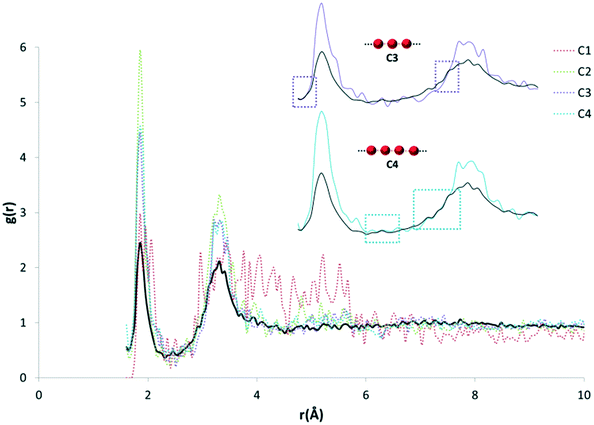
The purpose of recalculating RDFs for specific water motifs was to identify whether discrete features within the overall HW⋯OW RDF could be specific to a particular arrangement of water in organic hydrates observable in RDF plots. Initial analysis of the likelihood of this was performed by a simple overlay of each recalculated motif RDF with the original HW⋯OW RDF. It was found that peaks unique to the profile of particular motifs were also distinctly present in the original function. An example of this is shown in Fig. 5.

Fig. 5 An example of the initial overlay analysis of motif RDFs with the original HW⋯OW RDF. Discrete features for both the C3 (purple) and C4 motif (blue) appear to be present in the original function. Other discrete chain motifs are also represented here, as indicated by the legend (top right).

In order to quantify the likelihood of these distinct features correlating to the features present in the original RDF (omitting r < 1.6 Å), a statistical analysis of the goodness-of-fit (GOF) of each motif to the original RDF was conducted. The results of this analysis are shown in Table 1. The following statistical measures were employed; root mean squared error (RMSE), R², ln(L), the AIC, and BIC. Here, we treat the original RDF as the ‘true’ model, and the motif RDFs as approximating models.

From the results of AIC and BIC analysis, the GOF for each motif was ranked (the same ranking applies for both AIC and BIC), as shown in Table 1. It was found that the DC1 motif fitted most closely with the overall RDF. It might be expected that this would be the case, as DC1 motifs appear most frequently in our original dataset. However, a regression of the AIC and BIC scores against the frequency of occurrence for all motifs found no correlation to suggest this.

Qualitative interpretation of RDFs

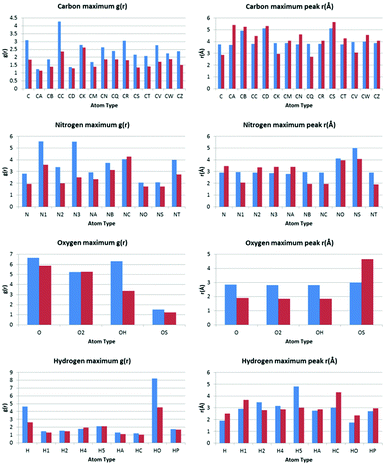
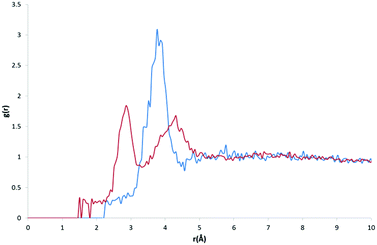
The values of g(r) and r found for each atom type are plotted against each other in bar charts in Fig. 6.

Fig. 6 The maximum peak (defined by g(r)) for each RDF pair profile (each atom type with HW and OW) was determined. These bar graphs show the g(r) value for the maximum peak of each atom type with OW (blue bars) and HW (red bars) on the left, with the distance at which these peaks were found plotted on the bar graphs on the right.

Comparison of the most prominent peak positions for each atom type with OW vs. each atom type with HW identifies whether, on average, the atom type is in closer proximity to the OW or HW of water. Comparison of the relative values of g(r) also gives an indication of which atom types are most likely to be in close proximity to water.

Carbon atom types

The calculated RDF profiles for carbon atom types generally show broad peak areas for pairs calculated with HW and OW, reflecting the lack of specific intermolecular interaction of water with carbon, and no definite orientation of water with respect to carbon. However, carbon atom types describing carbon in close proximity to an oxygen or nitrogen atom produced RDF profiles reflecting nearby interactions. For example, in the profile of the C atom type (Fig. 7), describing either an sp² carbonyl carbon or else an aromatic carbon with a hydroxyl substituent in tyrosine, the RDF maximum g(r) peak for C with HW occurs at lower r than the OW peak, indicative of the C–O⋯HW hydrogen bonding interaction (r = 2.86 Å; g(r) = 1.84). The profile also shows a secondary HW peak after an OW peak at r = 4.26 Å, with a separation of HW peaks = 1.40 Å, roughly corresponding to the average distance separating the hydrogens within a water molecule. This suggests that the average orientation of water in relation to C–O occurs with HW–OW along the C–O vector.

Fig. 7 RDF profiles for atom pairs for the C atom type with OW (blue) and HW (red).

A comparison of the profiles of the CC and the CK atom types (Fig. 8) gives an example of how using a sophisticated atom-typing algorithm may offer an advantage over using traditional element labels. Both atom types represent a carbon adjacent to a nitrogen in a five-membered ring. The CC atom type can have any substituent, whereas the CK atom type has a hydrogen substituent (see Fig. 1). The first immediate difference between the CC and CK RDFs is the overall likelihood of finding carbon to water pairs. The addition of a non-hydrogen substituent (i.e. in the CK RDF) produces a significant peak for CK⋯HW pairs that is not present in the CC⋯HW profile (r = 2.95 Å, g(r) = 2.63), as indicated by the peak highlighted in Fig. 8. This difference may seem intrinsic; however these results exemplify how the atom-typing method is able to describe the major differences in water distribution introduced in the average case of substituent changes. This again corroborates the postulate that atom typing algorithms are useful in a quantitative survey of hydrate distributions, as conventional atom labels based on atomic number alone would not have identified this change in distribution.

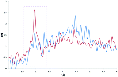Fig. 8 CC⋯HW RDF (blue) and CK⋯HW RDF (red) with a much larger peak apparent at ∼3 Å in the CK⋯HW profile (outlined in purple).

Where substituent effects are not considered, there is little more to be learned from the RDFs of carbon atom types, as the distribution of water around such atoms is expectedly broad, and does not show significant patterns which cannot be observed within the RDFs describing substituent atoms of terminal ligands.

Nitrogen atom types

The peak analysis of nitrogen atom types revealed a distinct difference in the profiles of nitrogen atoms participating in N–H⋯OW and N⋯HW interactions. The profiles of nitrogen groups participating in H-bond donor N–H⋯OW interactions show the highest g(r) OW peak to occur before the highest g(r) HW peak, as expected, and include the following atom types; N, N2, N3, NA and NT. Nitrogen atom types with profiles indicative of H-bond acceptor behaviour included N1, NB, and NC.

Oxygen atom types

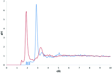
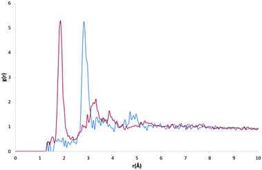
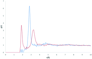
The peak analysis of oxygen atom type RDFs revealed more distinct differences in profiles than those found in nitrogen atom type RDFs. For two of the oxygen atom types, O (Fig. 9) and O2 (Fig. 10), representing carbonyl and carboxylate oxygen respectively, the overall profile of peaks were similar to those found for the H-bond acceptor groups in nitrogen atom type RDFs. The primary difference between the O and O2 RDFs is the comparative g(r) values of the HW and OW highest peaks. For the O atom type, the maximum g(r) value for OW is greater than for HW, whereas for the O2 atom type, both the OW and HW peaks have similar values of g(r).

Fig. 9 RDFs for the O atom type with OW (blue) and HW (red).

Fig. 10 RDFs for the O2 atom type with OW (blue) and HW (red).

The RDF profile for the OH (Fig. 11) atom type, representing alcohol oxygen, differs somewhat from the O and O2 atom types, reflecting the ability of an alcohol group to participate in both H-bond donor and acceptor interactions with water.

Fig. 11 RDFs for the OH atom type with OW (blue) and HW (red).

The first obvious difference in the OH RDF occurs for OH⋯HW pairs, where a definite intermolecular interaction is represented by a sharp and narrow peak. This peak represents the alcohol oxygen participating in H-bond acceptor behaviour, O⋯HW. Two further peaks are also present at r similar to those found in the O and O2⋯HW pair RDFs (r = 1.86 Å and 3.21 Å). These peaks are increasingly broadened, suggesting less definite positions and orientations of water as r increases. A high g(r) value peak occurs in the OH⋯OW RDF at r = 2.81 Å, which is the same r for the highest peak found in the O2⋯OW RDF, suggesting a similar mode of interaction.

Interestingly, for the OS atom type, the largest peak in the RDF for HW is found at a distance (∼4.6 Å) not indicative of hydrogen bond formation. The OS atom type represents an ether or ester oxygen. It is known that there few examples of ester hydrogen bonding in the CSD.³⁰ A study³¹ into ether and ester hydrogen bond formation found that ester oxygen hardly participates in hydrogen bonding. For (E)-esters, this is because of competition with the adjacent carbonyl group. For (Z)-esters, this is because of destabilisation due to a repulsive electrostatic interaction by the carbonyl group. Ethers were found to form hydrogen bonds at longer distances than expected, suggesting the bond is readily elongated by competing interactions.

Hydrogen atom types

Peak analysis of RDFs describing hydrogen atom type pairs with OW and HW revealed two distinct overall profiles. The first type of profile has sharp and narrow peaks, indicating direct interaction with water, with a well described average orientation of water around the respective atom types. The second profile shape represents no direct interaction of water with the respective hydrogen atom types, and presents as broad peaks at low values of g(r), suggesting fewer similarities between the pairs found in the structures used to build the RDFs, and less definition in the average orientation of water.

Only two of the nine investigated hydrogen atom types showed profiles with distinct narrow peaks; H, representing hydrogen in an amide or imino group, and HO, representing hydroxyl hydrogen. Both profiles indicate distinct H⋯OW pairs for interactions, characterised by the appearance of a peak in the hydrogen HW RDF before a hydrogen OW peak.

Future application

One example for the application of RDFs is for the improvement of the description of the first and second solvation shells in hydration free energy (HFE) calculations with the one-dimensional reference interaction site model (1D-RISM). A full description of RISM is available elsewhere,^32,33 but here we will discuss the application of RDFs to the calculation of HFEs.

Consider the following expression for HFE, as given by the RISM equations, employing a hypernetted chain closure (RISM-HNC);³⁴

where c_αγ(r) is the direct correlation function, and h_αγ(r) is the total correlation function. Usually, the total and direct correlation functions are unknown, and in order to find the HFE, RISM equations are used to find these correlation functions by integration over a grid. Thus, these expressions cannot be solved exactly, and g(r) is calculated from these correlation functions, with an additional term for the intermolecular pair potential using the HNC closure as;
where u is the intermolecular pair potential.

An appropriate weighting scheme, such as the atomic contribution to the solvent accessible surface area (SASA), can be applied to estimate the contribution of the RDF per atom to a total function g(r). It is worth noting that using the RDFs we have described here assumes that the solvent structure in solution is analogous to that in hydrate structures. This estimated distribution function could be used to solve the HNC closure to find the total and direct correlation functions. This could be implemented with either the typical Lennard-Jones type intermolecular pair potentials, or the PMF calculated from a SASA-weighted g(r). If the PMF is used for the pair potential, the energy expression simplifies to;

where h_αγ(r) = g(r) − 1. This simplification removes c_αγ(r) from the energy expression, thus this energy expression may neglect certain features of the system's interactions that are not well represented by the PMF, effectively assuming that there are no indirect correlations³³ between atom positions. However, this expression for the energy is extremely simple, and would be solved significantly quicker than the traditional calculations involving integration over a grid. Providing that the RDFs we have developed are applicable over a wide range of compounds and atom types, calculating HFEs with this method should offer an improvement upon a 1D-RISM calculation (with no additional corrections employed). Such methods are currently under development in our group. Promisingly, it has been previously found that using distribution functions calculated externally from the RISM methodology, for example from molecular dynamics, can improve HFEs calculated with the RISM energy terms.³⁵

Discussion & conclusions

The analysis of the contribution to the overall profile of water (via interpretation of HW⋯OW RDFs) of individual motifs of water within hydrate structures showed that discrete features appear in the RDFs, even at long distances. This is indicative of their ability to capture ‘real’ interactions. It was expected that long-range pair distances would mostly comprise noise, as an artefact of the most commonly occurring symmetrically equivalent atom positions; therefore the distinguishing of signal within these regions, attributable to particular arrangements of water, is promising for the application of RDFs in predictive methods in the future.

Acknowledgements

We are grateful for useful discussions with colleagues including Dr James McDonagh, and the groups of Professor Maxim Fedorov and Dr David Palmer. We thank the University of St Andrews, EPSRC (grant EP/L505079/1), and CCDC for funding and useful discussion. RES would also like to dedicate this article to the memory of the late Prof. Frank J. J. Leusen, who taught her computational chemistry as an undergraduate, and encouraged her continuation in the field, for which she is eternally grateful.

Notes and references

1. P. H. Wernet, D. Nordlund, U. Bergmann, M. Cavalleri, M. Odelius, H. Ogasawara, L. Å. Nalund, T. K. Hirsch, L. Ojamae, P. Glatzel, L. G. M. Pettersson and A. Nilsson, Science, 2004, 304, 995–999.
2. A. L. Gillion, N. Feeder, R. J. Davey and R. Storey, Cryst. Growth Des., 2003, 3, 663–673.
3. K. Fucke and J. W. Steed, Water, 2010, 2, 333–350.
4. J. L. Finney, J. Phys.: Conf. Ser., 2007, 57, 40–52.
5. K. Morris, in Polymorphism in Pharmaceutical Solids, ed. H. G. Brittain, Marcel Dekker, New York, 1999, pp. 125–181.
6. G. R. Desiraju, J. Chem. Soc., Chem. Commun., 1991, 426.
7. L. Infantes, L. Fabian and W. D. S. Motherwell, CrystEngComm, 2007, 9, 65.
8. J. van de Streek and S. Motherwell, CrystEngComm, 2007, 9, 55.
9. M. Mascal, L. Infantes and J. Chisholm, Angew. Chem., Int. Ed., 2005, 45, 32–36.
10. L. Infantes and S. Motherwell, CrystEngComm, 2002, 4, 454.
11. L. Infantes, J. Chisholm and S. Motherwell, CrystEngComm, 2003, 5, 480.
12. P. T. A. Galek, J. A. Chisholm, E. Pidcock and P. A. Wood, Acta Crystallogr., Sect. B: Struct. Sci., Cryst. Eng. Mater., 2014, 70, 91–105.
13. A. K. Soper, Chem. Phys., 2000, 258, 121–137.
14. P. Atkins and J. de Paula, Physical Chemistry for the Life Sciences, Oxford University Press, illustrate, 2011.
15. J. G. Kirkwood, J. Chem. Phys., 1935, 3, 300.
16. C. R. Groom, I. J. Bruno, M. P. Lightfoot and S. C. Ward, Acta Crystallogr., Sect. B: Struct. Sci., Cryst. Eng. Mater., 2016, 72, 171–179.
17. J. Wang, R. M. Wolf, J. W. Caldwell, P. Kollman and D. A. Case, J. Comput. Chem., 2004, 25, 1157–1174.
18. J. Wang, W. Wang, P. A. Kollman and D. A. Case, J. Mol. Graphics Modell., 2006, 25, 247–260.
19. J. Rodriguez-Carvajal and J. Gonzalez-Platas, Crystallographic Fortran Modules Library (CrysFML). A simple toolbox for crystallographic computing programs, Commission on Crystallographic Computing, IUCr, Newsletter No. 1, 2003, pp. 50–58.
20. M. I. Aroyo, J. M. Perez-Mato, E. T. D. Orobengoa, G. de la Flor and A. Kirov, Bulg. Chem. Commun., 2011, 43, 183–197.
21. M. I. Aroyo, J. M. Perez-Mato, C. Capillas, E. Kroumova, S. Ivantchev, G. Madariaga, A. Kirov and H. Wondratschek, Z. Kristallogr., 2006, 221, 15–27.
22. M. I. Aroyo, A. Kirov, C. Capillas, J. M. Perez-Mato and H. Wondratschek, Acta Crystallogr., Sect. A: Found. Crystallogr., 2006, 62, 115–128.
23. T. Hahn, International Tables for Crystallography: Volume A, Springer, 5th edn, 2005.
24. S. Le Roux and V. Petkov, J. Appl. Crystallogr., 2010, 43, 181–185.
25. M. P. Allen and D. J. Tildesley, Computer Simulation of Liquids, Oxford University Press, Oxford, 5th edn, 1991.
26. C. F. Macrae, I. J. Bruno, J. A. Chisholm, P. R. Edgington, P. McCabe, E. Pidcock, L. Rodriguez-Monge, R. Taylor, J. van de Streek and P. A. Wood, J. Appl. Crystallogr., 2008, 41, 466–470.
27. J. D. Bernal and R. H. Fowler, J. Chem. Phys., 1933, 1, 515.
28. A. Savitzky and M. J. E. Golay, Anal. Chem., 1964, 36, 1627–1639.
29. K. P. Burnham and D. Anderson, Model Selection and Multimodel Inference, Springer New York, New York, NY, 2nd edn, 2004.
30. K. Molcanov, B. Kojić-Prodić and N. Raos, Acta Crystallogr., Sect. B: Struct. Sci., 2004, 60, 424–432.
31. J. P. M. Lommerse, S. L. Price and R. Taylor, J. Comput. Chem., 1997, 18, 757–774.
32. R. E. Skyner, J. L. McDonagh, C. R. Groom, T. van Mourik and J. B. O. Mitchell, Phys. Chem. Chem. Phys., 2015, 17, 6174–6191.
33. E. L. Ratkova, D. S. Palmer and M. V. Fedorov, Chem. Rev., 2015, 115, 6312–6356.
34. S. J. Singer and D. Chandler, Mol. Phys., 1985, 55, 621–625.
35. H. Freedman and T. N. Truong, Chem. Phys. Lett., 2003, 381, 362–367.

---

Footnote

† Electronic supplementary information (ESI) available: All MATLAB scripts used to calculate the RDFs described, and the resulting RDFs, a list of refcodes for the crystal structures used, and a list of their measurement temperatures. See DOI: 10.1039/c6ce02119k

---