 Open Access Article
Creative Commons Attribution 3.0 Unported Licence
Nonlinear elasticity of semiflexible filament networks
Fanlong
Meng
and
Eugene M.
Terentjev
*
Cavendish Laboratory, University of Cambridge, Cambridge, CB3 0HE, UK. E-mail: emt1000@cam.ac.uk
First published on 8th July 2016
Abstract
We develop a continuum theory for equilibrium elasticity of a network of crosslinked semiflexible filaments, spanning the full range between flexible entropy-driven chains to stiff athermal rods. We choose the 3-chain constitutive model of network elasticity over several plausible candidates, and derive analytical expressions for the elastic energy at arbitrary strain, with the corresponding stress–strain relationship. The theory fits well to a wide range of experimental data on simple shear in different filament networks, quantitatively matching the differential shear modulus variation with stress, with only two adjustable parameters (which represent the filament stiffness and the pre-tension in the network, respectively). The general theory accurately describes the crossover between the positive and negative Poynting effect (normal stress on imposed shear) on increasing the stiffness of filaments forming the network. We discuss the network stability (the point of marginal rigidity) and the phenomenon of tensegrity, showing that filament pre-tension on crosslinking into the network determines the magnitude of linear modulus G0.
1 Introduction
Networks of semiflexible filaments and fibers are common in biological systems, where dynamic structures of tunable strength, elasticity, and adjustable response are required.1–3 From the microscopic scale of cytoskeleton to the macroscopic scale of fibrous tissue, such networks utilize stiff or semiflexible filaments, allowing for rich mechanical response,4 dynamic remodelling,5,6 and controlled structural failure,7 while remaining an open structure allowing easy through access for solvents and solutes.8 Inspired by these observations, filament networks are produced in industry, and now stand as a promising area in manufacturing functional materials.9,10The physics of a single semiflexible chain or filament is well understood with the aid of worm-like chain model, in various implementations and approximations.11–15 The full theory is capable of accurately describing the force-extension relationship, as well as the magnitude of transverse fluctuations, for a range of filament stiffness spanning from very high (a rigid elastic rod) to very flexible (a classical polymer coil) and a range of end-to-end extensions from zero up to the full stretch where the entropic force has a characteristic divergence. When such filaments form a macroscopic crosslinked network, the main scaling features of its nonlinear mechanical response are still determined by the single filament properties, as reviewed in ref. 16 and 17. There have been many key contributions to the elastic theory of stiff and semiflexible networks, including ones highlighting the issues of strain non-affinity.18,19
In order to obtain the constitutive relationship of a semiflexible network, a widely used approach follows the following procedure (explained in detail in chapters 3 and 4 of ref. 20): the shear stress on ij plane is calculated by summing the contributions of the tension along the i axis of all the chains crossing the j plane. This approach has been very successful in deriving viscoelastic properties of polymer solutions and melts under shear flow;20,21 Storm et al.22 have applied the same stress–strain relation to a crosslinked network by assuming the affine elastic strain acting on each filament and the probability distribution of semiflexible filament length of Wilhelm and Frey.23 This model qualitatively describes how the network behaves when being deformed; however, it can only be used numerically (since no closed expressions are possible) and it omits the pre-stress acting on the chains, as in this model the tension is assumed as zero when there is no deformation. Wilhelm and Frey also produced a numerical simulation of filament network elasticity on their own,24 using the Mikado model of connectivity and athermal rigid rods as elastic elements. Although important issues of percolation rigidity threshold are exposed, this work cannot be used to describe most experimentally relevant (and most biological) filaments. More recently, Palmer and Boyce25 proposed a closed analytical form of elastic free energy, with the corresponding constitutive relation, using the same force-extension filament relationship as Storm et al. They applied the ‘8-chain model’ originally introduced in the context of ordinary rubber elasticity25 with an approximate expression for individual filament elasticity applied for each strand. This might be the best attempt in formulating the nonlinear elasticity of semiflexible network to date. On the other hand, Unterberger et al.26 developed a ‘1-chain’ model for a network, by assuming filaments have a homogenous orientational distribution in the equilibrium system, and the average (imposed) stretch of the network λ is a p-root average of deformations of individual filaments:  , where λ*(θ,ϕ) is the deformation of an individual filament, p is the averaging parameter and A the area of the unit sphere. This procedure allows the local stretch to fluctuate around its average value, and may partly account for the non-affinity. This model could only be applied numerically to reproduce several key mechanical features (shear and normal stress).
Most good models discussed here make a successful fitting of shear stress data of different filament networks, which captures the generic stress-stiffening effect originating from the characteristic divergence of the force-extension curve of an individual filament. Usually, the authors employ the versions of celebrated Marco–Siggia interpolation formula,12 which gives the correct response for filaments near full-extension (but much less so for more flexible filaments). In fact, the well-known MacKintosh scaling of differential shear modulus with stress, K ∝ σ3/2, in the stress-stiffening regime is entirely based on the mentioned divergence of an individual filament near full extension27 (it holds even for an athermal network of undulating filaments, as long as the tensile force is proportional to the inverse-square of the compression, as is the case near full extension28,29). Therefore, a mere agreement (good fitting) of shear stress–strain curves is not a sufficient test of different theories. In particular, they must simultaneously describe the effect of negative normal stress in the network of stiffer filaments, with a positive normal stress (also known as the Weissenberg effect) for networks made of more flexible chains.30,31 It turns out that none of the mentioned theories, including the 8-chain model of Palmer and Boyce, are able to produce the correct normal stress, or address the network stability increasing with filament pre-tension.32 In this paper we develop and discuss a continuum theory of semiflexible network (in closed analytical form) that addresses these issues, while retaining accurate fitting of a wide range of shear stress data.
2 Network theory
Before introducing free energy of a semiflexible network, we need to discuss the properties of a single semiflexible filament. A filament connecting two neighboring crosslinks in a network is sketched in Fig. 1(a), with coordinates r(s), where 0 ≤ s ≤ Lc is the arc-length coordinate along the chain. Different approaches to the chain (in)extensibility have been tested over the years,33 from the strict constraint to the requirement that the length of filament remains constant on average (while small local fluctuations are allowed),15,23 to the models that explicitly include filament stretching.22,34 It turns out that in the regime of high extension, when there are no foldbacks (hairpins) on the chain, all length-constraining models give the same divergence of the force-extension, f ∝ 1/(1 − x)2, with the end-to-end ratio x = ξ/Lc, where ξ is the end-to-end length of the filament, Fig. 1(a). This was used by the famous interpolation formula of Marko and Siggia.12 More recently, a complete theory of filament entropic elasticity has been developed, which spans the full range of extensions and the full range of bending modulus.15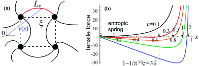 | ||
| Fig. 1 (a) A sketch of semiflexible network mesh unit, with a bent filament connecting two crosslinks with its contour length Lc, and end-to-end length ξ being the mesh size. (b) The relationship15 between the tensile force, f(x)/kBT, and end-to-end factor, x = ξ/Lc, plotted for semiflexible chains with different stiffness c, and marking the position x0 for a chain to stay at the force-free state. | ||
In the worm-like chain model,11,35 the bending energy can be expressed by  , where κ is the bending rigidity. The key physical quantity for describing the stiffness of a polymer chain is the persistence length lp = κ/kBT. When the contour length of the filament, Lc, is comparable with its persistence length lp, the chain is regarded as “semiflexible”. Combining the effects of enthalpy arising from bending and entropy of conformation fluctuations, the closed form of the single chain free energy15 can be expressed as a function of its end-to-end factor, x = ξ/Lc:
 | (1) |
As shown in Fig. 1(b), if the value of c is smaller than a critical value c* = π−3/2 ≈ 0.18, the minimum of the free energy (or the force-free natural length) will be at x = 0; such a chain can be regarded as flexible. When c ≪ c*, one recovers the Gaussian entropic spring form: Fchain ≈ (2kBT/πlpLc)ξ2. The Marko–Siggia (in fact, Fixman–Kovac) limit commonly used for quick fitting of force-extension curves is reached for flexible chains at high extension c ≪ c*, x → 1: Fchain ≈ (kBT/πlpLc)/(1 − x). When c ≫ c*, the chain can be regarded as a stiff rod with a natural length  , and its energy is dominated by elastic bending: Fchain ≈ (π2κ/Lc)[1 − x]. Under compression x < x0 such a filament undergoes Euler buckling instability. Note that on forming a crosslinked network, x does not need to be equal to x0 for each strand in equilibrium, meaning there can be pre-tension in the network.
We now construct the continuum elastic free energy of a network of such filaments using the methodology that was successfully developed in rubber elasticity.36,37 If the sample shape is changed with a deformation tensor E, then the corresponding Cauchy–Green tensor38 is C = EET, with eigenvalues: λ12, λ22 and λ32. The values λ1, λ2, λ3 can be interpreted as stretching ratios along the principal directions of deformation. A class of simple, yet powerful theories of rubber elasticity is formulated in terms of invariants of the C–G tensor, I1 = λ12 + λ22 + λ32, I2 = λ12λ22 + λ22λ32 + λ32λ12 and I3 = λ12λ22λ32. Famous examples of this class are neo-Hookean (Gaussian), Mooney-Rivlin, and Gent models (see ref. 39 for review). Note that polymer networks are frequently treated as incompressible, so I3 = 1.
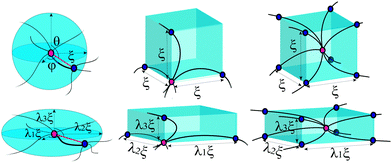
For a polymer network, the chains are distributed and crosslinked randomly throughout the material, which is the main difficulty in obtaining an analytical expression of the total free energy of the network (unless the individual chain is Gaussian). To incorporate a more complicated chain, such as eqn (1), into a constitutive framework, it is necessary to have a model that relates the chain deformation to the applied affine strain. This can be accomplished by representing an element of volume in the average network as a “mesh cell”, which is then symmetrically multiplied to fill the volume. Here we need to distinguish “affinity” and “non-affinity” in a filament network constructed by the unit-cell method. A “mesh cell” is deformed differently from the material, as these cells are constructed in orientation aligned with the principal stretching direction of the material, which is referred to as “non-affinity” by Palmer and Boyce.25 All mesh cells deform in the same way, with repeated deformed structure. However, the real non-affinity can arise from the different responses among different “mesh cells”, due to local force relaxation. In this work we refer to the concepts of “affinity” or “non-affinity” in the local context of individual filament junctions and mesh cells, rather than the global one between the orientation of a mesh cell and the macroscopic deformation of the material. In assuming a symmetry of repeated mesh cells, we automatically discard the effects of the local non-affine deformations,40,41i.e. take all mesh cells deforming uniformly, which we know must be the case at least for stiff filaments.18,19 Since there is no quantitative way of assessing the degree of the error introduced by the affine approximation (in our interpretation), we will have to look at the fits to the experimental data for validation. Within a mesh cell, chains or crosslinks have several possible arrangements, reflecting what one assumes about the topology of the network mesh, see Fig. 2. Most acceptable structures include the homogeneous sphere (HS) in 1-chain network model, the primitive cubic (PC) in 3-chain model, tetrahedral (TH) in 4-chain model, and body-centered cubic (BCC) in 8-chain model (see ref. 25 and a review36 for detail).
In 1-chain model,15,26,36 one end of a polymer chain is fixed at the center of a sphere, while the other end is on the sphere surface at an arbitrary orientation (θ,φ), distributed isotropically. When deformed by E, with stretching ratios along principal directions λ1, λ2, and λ3, the lengths of the three semi-axes will change from ξ, to ξλ1, ξλ2 and ξλ3, respectively. The elastic energy density of the network can be expressed as an orientational average of a deformed filament:
 | (2) |
 . If one takes the ‘entropic spring’ limit of the Gaussian chain, the average F1c reduces to the classical neo-Hookean rubber-elastic expression nkBT(2ξ2/3πlpLc)[λ12 + λ22 + λ32].
However, in the general case the free energy in 1-chain model cannot be expressed in analytical form as a function of strain invariants, which renders it less convenient. In the following, we compare the 3- and 8-chain models, and decide on the 3-chain model preference, in particular due to the failure of 8-chain model in reproducing the normal stress.
In the 3-chain model, a primitive cubic is constructed with lattice points representing the crosslinking sites, and the edges are aligned along the principle directions of deformation tensor E. Three chains are linked with their end-to-end vectors along the edges and the equilibrium mesh size ξ. On deformation, the lengths of three perpendicular edges at one lattice point become λ1ξ, λ2ξ and λ3ξ, respectively. Then the free energy density of a semiflexible network can be expressed as
 | (3) |
 | (4) |
The body-centered cubic cell of 8-chain model is constructed with eight filaments connected from the center point to all eight lattice points.25 The edges of the cell are ξ as we define the mesh size, while the chains are shorter by factor  . The important feature of the high-symmetry 8-chain model is that on deformation all chains change their distance by exactly the same amount, from
  to simply
  , since the mesh cell is aligned along the principal axes of deformation tensor E. The free energy density of the network in this case is given by the single-chain expression directly:
 | (5) |
When the elastic energy is expressed as a function of strain invariants, the stress tensor of an incompressible material (with I3 = 1) can be obtained as:38,39
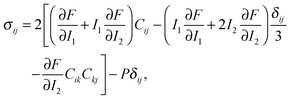 | (6) |
3 Simple shear deformation
Let us consider the simple shear deformation such that in Cartesian coordinates a point (x, y, z) in an original material will change to (x + γz,y,z) after being sheared; γ is the shear strain. The incompressibility is satisfied automatically, and the remaining strain invariants are: I1 = I2 = 3 + γ2. The shear stress in 3-chain model can be obtained from the general constitutive relation (6) as: | (7) |
 | (8) |
Take actin and fibrin network under simple shear deformation as an example. Both 3-chain and 8-chain models fit the shear-experiment data from ref. 22 and 27 equally well, in fact – perfectly, as shown in Fig. 3(a). The stiffness, c, and the initial end-to-end factor, x = ξ/Lc, obtained by fitting with 3-chain model are a bit smaller than those in 8-chain model, but both in the semiflexible regime. This is because the eight chains in a BCC are stretched equally (in principal axes) and share the deformation, while the three chains in a PC are stretched differently and the most stretched one contributes the most to the nonlinear elastic energy. We believe the intrinsic heterogeneity in the 3-chain model, and the fact that the chain lying along the maximum principle stretch direction dominates the response of the whole cubic in semiflexible networks, is closer to the realistic case of filament network. In addition, we shall see below that the 8-chain model cannot explain negative normal stress. Hence we apply the 3-chain model in the following. Fig. 3(b) shows fits to experimental data for a wide variety of semiflexible filaments. In this figure we plot the shear modulus G(γ) instead of stress, because the fitting convergence is much better when the initial data section is close to 1. Fitted parameters (c,x) are listed in Table 1 below, along with other parameters for each material that we list from the literature.
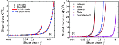 | ||
| Fig. 3 (a) Fitting stress–strain experimental data of sheared actin27 and fibrin network22 with 3-chain model (red curve) and 8-chain model (blue curve). (b) Fitting curves of experimental data22 for sheared actin, collagen, vimentin, fibrin and neurofilament networks are optimally obtained for the scaled ratio G(γ)/G0, which has a limit of 1 at γ → 0; the fitting parameters for 3-chain model are given in Table 1. | ||
First of all, one may be surprised that the persistence length of collagen fibers is quoted as 20 μm, when there is a large body of literature that would claim that collagen fibers are stiff athermal rods with persistence length of centimeters. This is all to do with the way a sample is prepared, and we use/quote the data42 where the collagen was apparently less aggregated than in a typical extra-cellular matrix. The same ambiguity will apply to actin networks as well, below. Another point to note about the fitted values in Table 1 is about neurofilament, which has c < c*, that is, rather flexible chains. Taking the fitted value for x = 0.15 = ξ/Lc, this means that Lc in this network was ∼1.6 μm, i.e. about 3.6 times longer than lp. By calculating  for different filaments listed in Table 1, we see that the fitted x is smaller than x0, indicating all of the filaments in Fig. 3(b) are pre-compressed, rather than pre-stretched in the equilibrium state of the network.
As Table 1 shows, no matter what the effective stiffness of the examined biofilaments, the ratio of fitted parameters c/x = lp/2ξ remains close to 1. Later, when we discuss the network stability (Fig. 6), it will become clear that all the networks we examined here lie very near the stability boundary. It is not clear to us whether the fact that the mesh size is close to the filament persistence length is an unintended result of different crosslinking density in experiments,22 or is a relevant and universal biological feature.
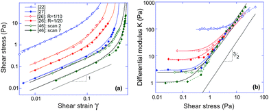
It is clear that networks of biological filaments have a great variety even within the same substance. Fig. 4 shows the published data for in vitro crosslinked actin networks reported by different groups, all performing the simple-shear experiment (the data is digitized from references given in the plot). The stress–strain plotted in log–log format allows a clear identification of the linear regime σ = G0γ (the modulus varying between 95 Pa and 1 Pa for different sets), and the subsequent stiffening at higher shear. All curves in Fig. 4(a) are fitted by the same eqn (7) with the linear modulus G0 and the two parameters (c,x) taking values: 95 Pa, (1.43, 0.86); 14.8 Pa, (1.37, 0.85); 7.5 Pa, (0.94, 0.80); 3.0 Pa, (0.38, 0.80); 2.5 Pa, (0.38, 0.75) and 1.0 Pa, (0.27, 0.74) for the six sets from top to bottom. The difference between two data sets from ref. 26 is the density of heavy meromyosin (HMM) crosslinker (labelled on the plot); the difference between two data sets from ref. 46 is the degree of actin filament bundling: an initial network of F-actin filaments turned into a more sparse collection of bundles under repeated shear cycles.46 As a result the network at ‘cycle 7’ has lower G0 but higher stiffening.
To find the onset of non-linearity in our theory, the differential shear modulus K(γ) can be expanded in powers of shear strain γ:
 | (9) |
 . The stress at this point is
  . This crossover stress σt increases with the temperature as (kBT)2/κ, closely matching experimental observations.47 At the end of range, when the shear strain approaches the point of divergence in stress σxz, (γ → 1/x − x in eqn (7)), the stress and the differential modulus can be approximated as:
 | (10) |
 | (11) |
One has to make a comment here, in the context of K ∼ σ3/2 scaling and different experiments. In many cases, such as in Unterberger et al.,26 the actin network was crosslinked by HMM and apparently retains some transient activity, producing the stress-softening and plasticity at higher stress (this is also the case in ref. 46 before the actin filaments formed bundles, or with F-actin crosslinked by filamin). Of course, our theory is not intended to deal with network plasticity (we assumed all crosslinks permanent) and therefore we only retained the experimental data points in the early stress-stiffening regime to see the 3/2 scaling.
On the other hand, just by examining the actual data for the actin network of Storm et al.,22 one might conclude that it strongly and systematically deviates from the 3/2 scaling. In fact, the authors of ref. 22 develop their own theory invoking various additional factors (e.g. filament extensibility) to account for this deviation. However, our basic theory, assuming permanent crosslinks, bulk incompressibility and inextensible filaments, evidently fits both σ(γ) and K(σ) data very well. The fact that the data (and the predicted curve) do not appear to follow the 3/2 scaling is due to the fact that, for these values of c and x, the final crossover to this characteristic scaling regime would occur at an even higher stress (at which point the network would probably not survive in practice).
4 Normal stress
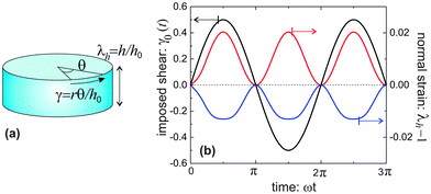
Though simple shear deformation was helpful in this analysis, the important issue of normal stress remains controversial. This is mainly because of the uncertain boundary conditions, see ref. 51 for detail. Since the experiments reporting normal stress measurements are most commonly conducted in rotating cylindrical geometry of a standard rheometer,30,31 we will consider this geometry and realistic boundary conditions to describe the response of the material in its normal direction when a shear is applied, as shown in Fig. 5(a). Suppose the height and the radius of the undeformed cylinder are h0 and R0, respectively; on deformation they may become h = λhh0 and R = λRR0. Incompressibility maintains λhλR2 = 1. In the (r, θ, z) coordinate system, after rotating the top plate by the angle Θ, the coordinates change as: :
: | (12) |
 | (13) |
Fig. 5(b) shows the results for equilibrium λh, presented as a response to an oscillating imposed shear γ0, for two model materials with different filament stiffness and pre-tension. A flexible network (c = 0.1, x = 0.1) has a positive Poynting effect, or positive normal stress is required to counter the expansion along the height (in other setting, this is called the Weissenberg effect). In a flexible network (c < c*), when the mesh size is much smaller than the contour length of the subchains connecting the neighboring crosslinks, i.e., x0 ≪ 1, the entropic energy plays a main role. Though chains are stretched along the principal extension direction in the shear geometry illustrated in Fig. 5(a), the chains in other two principle directions are more likely being compressed, leading to the material contraction along the radial and circumferential directions. However, if the mesh size is comparable with the contour length of the subchains, 0 ≪ x0 < 1, the material can behave in a negative Poynting effect manner: the height of the cylindrical sample contracts, or negative normal stress is required to counter that and maintain the fixed height. This is because the force acting on the chains directed along the principal extension in Fig. 5(a) is close to a divergence if x0 → 1, and it causes less energy when the material is compressed in the longitudinal direction, rather than stretched. Similar reason works also for a network of more stiff filaments (see blue curve for c = 0.3 > c*, x = 0.6).
We did not specifically calculate the normal stress here (this would be a cumbersome process involving the full tensor form of eqn (6), first fixing the pressure P from the condition of zero radial stress on the free outer surface). However, the magnitude of normal stress can be easily estimated from the linear relationship σh ∼ 3G0(λh − 1), which uses the fact that the normal strain is quite small (i.e. the linear regime is justified) and the Young modulus is 3G0. Taking the fibrin values in Table 1 as an example, the normal stress is about 11.5 Pa under a shear strain of γ0 = 0.5. These are very close to the observations in experiments.30,31 The magnitude of σh ≃ 20 Pa for the same shear also accurately matches the actin results obtained in ref. 26.
Fig. 6 gives the full ‘phase diagram’ of the stiffness-tension parameter space (c,x) with phase boundaries separating positive/negative normal stress regions. In order to generate this diagram, for each parameter set (c,x) we have calculated the value of λh by minimizing F(λh;γ0), under the given shear. In this way the boundary separating the positive (λh > 1, σh > 0) and the negative (λh < 1, σh < 0) normal stress regions in Fig. 6 is calculated. There is also a weak dependence of this boundary on the magnitude of the applied shear strain, which is due to the inherent non-linearity of stress–strain response; however, we are not showing this in the figure to avoid clutter.
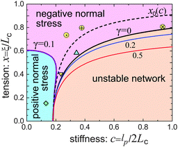 | ||
| Fig. 6 The phase diagram of the network response at different stiffness, c, and filament pre-tension, x, showing the boundaries of positive/negative Poynting effect and the boundary of network stability (the dashed line of the neutral filament, x0, was defined in Fig. 1). Three ‘softer’ filament networks from Table 1 are shown in this map: Δ-vimentin, ∇-fibrin, and ◇-neurofilament networks. Three actin networks from Fig. 4 also fit on this map: ⊕-,27 ⊗-,26 and ⊙-.46 | ||
Fig. 6 shows that a loose flexible network usually has a positive Poynting effect, while a network of more stiff filaments has a negative Poynting effect, especially when the filaments are crosslinked with increasing pre-tension.
5 Network stability
One can see from Fig. 3(b) and 4(b) that the linear regime when σ = G0γ persists for a different range of strain in different filaments; the onset of hyperelastic regime is determined by how much pre-tension is in the filaments, i.e. how x compares with x0(c) from eqn (1). The linear shear modulus G0 can be easily obtained from our theory: in 3-chain model it is given by the first term in eqn (9). The marginal rigidity condition G0 ≥ 0 determines the strand pre-tension that is required for achieving a stable network. The stability criterion here is: | (14) |
The stability boundary of the network is plotted in Fig. 6. The condition for G0 = 0 gives the equilibrium case labelled as γ = 0 in the phase diagram. However, the full analysis shows that the magnitude of the shear strain modifies the stability condition, as represented by the coloured curves for γ = 0.2 and 0.5. This shift means that the region of mechanical stability of filament network expands on increasing deformation, which matches exactly what the recent paper by Sharma et al. states.32
To summarize, in this work we develop a continuum elastic theory of a network of semiflexible filaments, by implementing the general free energy of one semiflexible chain into that of a disordered network. On reflection, we choose the 3-chain model as most closely matching the realistic system – and achieve various quite stringent fits for a number of different experimental data sets over the full range of nonlinear stress–strain range. We demonstrate that the general theory produces the conditions for positive/negative Poynting effect (normal stress) in a network under imposed shear. The greatest weakness of this model is omitting the effects of local strain non-affinity, which might play an important role when crosslink density of the network is small and filaments stiff. However, the very broad agreement of our affine theory with so many different experiments is reassuring. The effect of tensegrity, or linking of filament pre-tension to the network stability and the magnitude of the shear modulus G is an unexpected result of this theory. We believe that the presented analytical continuum model can provide as an efficient and portable tool for studying the mechanical properties of semiflexible networks.
Acknowledgements
This work has been funded by the TCM Critical Mass Grant from EPSRC (EP/J017639). We are grateful for informative discussions with Masao Doi and Zhongcan Ouyang, and thank Cornelius Storm for providing their raw experimental data.22References
- B. Wickstead and K. Gull, J. Cell Biol., 2011, 194, 513–525 CrossRef CAS PubMed.
- G. Faury, Pathol. Biol., 2001, 49, 310–325 CrossRef CAS PubMed.
- S. Özbek, P. G. Balasubramanian, R. Chiquet-Ehrismann, R. P. Tucker and J. C. Adams, Mol. Biol. Cell, 2010, 21, 4300–4305 CrossRef PubMed.
- K. E. Kasza, A. C. Rowat, J. Liu, T. E. Angelini, C. P. Brangwynne, G. H. Koenderink and D. A. Weitz, Curr. Opin. Cell Biol., 2007, 19, 101–107 CrossRef CAS PubMed.
- P. Bursac, G. Lenormand, B. Fabry, M. Oliver, D. A. Weitz, V. Viasnoff, J. P. Butler and J. J. Fredberg, Nat. Mater., 2005, 4, 557–561 CrossRef CAS PubMed.
- D. A. Fletcher and R. D. Mullins, Nature, 2010, 463, 485–492 CrossRef CAS PubMed.
- X. Trepat, G. Lenormand and J. J. Fredberg, Soft Matter, 2008, 4, 1750–1759 RSC.
- T. Lecuit, P.-F. Lenne and E. Munro, Annu. Rev. Cell Dev. Biol., 2011, 27, 157–184 CrossRef CAS PubMed.
- E. W. Wong, P. E. Sheehan and C. M. Lieber, Science, 1997, 277, 1971–1975 CrossRef CAS.
- M. R. Falvo, G. J. Clary, R. M. Taylor, V. Chi, F. P. Brooks, S. Washburn and R. Superfine, Nature, 1997, 389, 582–584 CrossRef CAS PubMed.
- M. Fixman and J. Kovac, J. Chem. Phys., 1973, 58, 1564–1568 CrossRef CAS.
- J. F. Marko and E. D. Siggia, Macromolecules, 1995, 28, 8759–8770 CrossRef CAS.
- B. Y. Ha and D. Thirumalai, J. Chem. Phys., 1996, 106, 14 Search PubMed.
- C. Bouchiat, M. D. Wang, J.-F. Allemand, T. Strick, S. M. Block and V. Croquette, Biophys. J., 1999, 76, 409–413 CrossRef CAS PubMed.
- J. R. Blundell and E. M. Terentjev, Macromolecules, 2009, 42, 5388–5394 CrossRef CAS.
- F. C. MacKintosh, Cytoskeletal mechanics: models and measurements, Cambridge University Press, Cambridge, 2006 Search PubMed.
- C. P. Broedersz and F. C. Mackintosh, Rev. Mod. Phys., 2014, 86, 995–1036 CrossRef CAS.
- D. A. Head, A. J. Levine and F. C. MacKintosh, Phys. Rev. Lett., 2003, 91, 108102 CrossRef PubMed.
- C. Heussinger, B. Schaefer and E. Frey, Phys. Rev. E: Stat., Nonlinear, Soft Matter Phys., 2007, 76, 031906 CrossRef PubMed.
- M. Doi and S. F. Edwards, The theory of polymer dynamics, Oxford University Press, Oxford, 1986 Search PubMed.
- D. C. Morse, Macromolecules, 1999, 32, 5934–5943 CrossRef CAS.
- C. Storm, J. J. Pastore, F. MacKintosh, T. Lubensky and P. A. Jamney, Nature, 2005, 435, 191–194 CrossRef CAS PubMed.
- J. Wilhelm and E. Frey, Phys. Rev. Lett., 1996, 77, 2581–2584 CrossRef CAS PubMed.
- J. Wilhelm and E. Frey, Phys. Rev. Lett., 2003, 91, 108103 CrossRef PubMed.
- J. S. Palmer and M. C. Boyce, Acta Biomater., 2008, 4, 597–612 CrossRef PubMed.
- M. J. Unterberger, K. M. Schmoller, A. R. Bausch and G. A. Holzapfel, J. Mech. Behav. Biomed. Mater., 2013, 22, 95–114 CrossRef CAS PubMed.
- M. L. Gardel, J. H. Shin, F. C. MacKintosh, L. Mahadevan, P. Matsudaira and D. A. Weitz, Science, 2004, 304, 1301–1305 CrossRef CAS PubMed.
- T. Van Dillen, P. Onck and E. Van der Giessen, J. Mech. Phys. Solids, 2008, 56, 2240–2264 CrossRef CAS.
- G. Žagar, P. R. Onck and E. Van Der Giessen, Macromolecules, 2011, 44, 7026–7033 CrossRef.
- P. A. Janmey, M. E. McCormick, S. Rammensee, J. L. Leight, P. C. Georges and F. C. MacKintosh, Nat. Mater., 2007, 6, 48–51 CrossRef CAS PubMed.
- H. Kang, Q. Wen, P. A. Janmey, J. X. Tang, E. Conti and F. C. MacKintosh, J. Phys. Chem. B, 2009, 113, 3799–3805 CrossRef CAS PubMed.
- A. Sharma, A. J. Licup, K. A. Jansen, R. Rens, M. Sheinman, G. H. Koenderink and F. C. MacKintosh, Nat. Phys., 2016, 12, 584–587 CrossRef CAS.
- M. Otto, J. Eckert and T. A. Vilgis, Macromol. Theory Simul., 1994, 3, 543–555 CrossRef CAS.
- D. C. Morse, Macromolecules, 1998, 31, 7030–7043 CrossRef CAS.
- O. Kratky and G. Porod, Recl. Trav. Chim. Pays-Bas, 1949, 68, 1106–1122 CrossRef CAS.
- M. C. Boyce and E. M. Arruda, Rubber Chem. Technol., 2000, 73, 504–523 CrossRef CAS.
- L. R. G. Treloar, The physics of rubber elasticity, Oxford University Press, Oxford, 1975 Search PubMed.
- A. F. Bower, Applied mechanics of solids, CRC press, Boca Raton, 2009 Search PubMed.
- C. O. Horgan, Intl. J. Non-Lin. Mech., 2015, 68, 9–16 CrossRef.
- A. Zaccone, J. R. Blundell and E. M. Terentjev, Phys. Rev. B: Condens. Matter Mater. Phys., 2011, 84, 174119 CrossRef.
- C. P. Goodrich, A. J. Liu and S. R. Nagel, Nat. Phys., 2014, 10, 578–581 CrossRef CAS.
- A. M. Stein, D. A. Vader, L. M. Jawerth, D. A. Weitz and L. M. Sander, J. Microsc., 2008, 232, 463–475 CrossRef PubMed.
- F. Gittes, B. Mickey, J. Nettleton and J. Howard, J. Cell Biol., 1993, 120, 923–934 CrossRef CAS PubMed.
- N. Mücke, L. Kreplak, R. Kirmse, T. Wedig, H. Herrmann, U. Aebi and J. Langowski, J. Mol. Biol., 2004, 335, 1241–1250 CrossRef.
- O. I. Wagner, S. Rammensee, N. Korde, Q. Wen, J. F. Leterrier and P. A. Janmey, Exp. Cell Res., 2007, 313, 2228–2235 CrossRef CAS PubMed.
- K. Schmoller, P. Fernandez, R. Arevalo, D. Blair and A. Bausch, Nat. Commun., 2010, 1, 134 CrossRef CAS PubMed.
- P. H. J. Kouwer, M. Koepf, V. Le Sage, M. Jaspers, A. M. van Buul, Z. H. Eksteen-Akeroyd, T. Woltinge, E. Schwartz, H. J. Kitto, R. Hoogenboom, S. J. Picken, R. J. M. Nolte, E. Mendes and A. E. Rowan, Nature, 2013, 493, 651–655 CrossRef CAS PubMed.
- M. L. Gardel, J. H. Shin, F. C. MacKintosh, L. Mahadevan, P. A. Matsudaira and D. A. Weitz, Phys. Rev. Lett., 2004, 93, 188102 CrossRef CAS PubMed.
- Y. C. Lin, N. Y. Yao, C. P. Broedersz, H. Herrmann, F. C. MacKintosh and D. A. Weitz, Phys. Rev. Lett., 2010, 104, 058101 CrossRef PubMed.
- Y. C. Lin, C. P. Broedersz, A. C. Rowat, T. Wedig, H. Herrmann, F. C. MacKintosh and D. A. Weitz, J. Mol. Biol., 2010, 399, 637–644 CrossRef CAS PubMed.
- C. O. Horgan and J. G. Murphy, J. Elastoplast., 2010, 98, 205–221 CrossRef.
- L. A. Mihai and A. Goriely, Proc. R. Soc. A, 2011, 467, 3633–3646 CrossRef.
- J. H. Poynting, Proc. R. Soc. A, 1909, 82, 546–559 CrossRef.
- D. E. Ingber, Annu. Rev. Physiol., 1997, 59, 579–599 CrossRef PubMed.
| This journal is © The Royal Society of Chemistry 2016 |

