DOI:
10.1039/C5SM02965A
(Paper)
Soft Matter, 2016,
12, 3737-3749
Dynamics of flexible active Brownian dumbbells in the absence and the presence of shear flow
Received
8th December 2015
, Accepted 26th February 2016
First published on 1st March 2016
Abstract
The dynamical properties of a flexible dumbbell composed of active Brownian particles are analytically analyzed. The dumbbell is considered as a simplified description of a linear active polymer. The two beads are independently propelled in directions which change in a diffusive manner. The relaxation behavior of the internal degree of freedom is tightly coupled to the dumbbell activity. The latter dominates the dynamics for strong propulsion. As is shown, limitations in bond stretching strongly influence the relaxation behavior. Similarly, under shear flow, activity determines the relaxation and tumbling behavior at strong propulsion. Moreover, shear leads to a preferred alignment and consequently to shear thinning. Thereby, a different power-law dependence on the shear rate compared to passive dumbbells under flow is found.
1 Introduction
The constituents of active matter convert internal chemical energy or utilize energy from their environment for their propulsion.1 The resulting nonequilibrium dynamical behavior gives rise to rich physical phenomena, such as swarming,2–6 turbulence,5 activity-induced clustering, and phase transitions.7–20 The spectrum of biologically active systems is wide and ranges from moving bacteria,1,21,22 the cytoskeleton in living cells22–31 to the macroscopic scale of flocks of birds and mammalian herds.32 For synthetically active particles, chemical or physical propulsion mechanisms are exploited for spherical colloids8,33–35 or objects of other shapes.35,36 Various propulsion strategies are realized in nature. Bacteria are typically propelled by one or several flagella.1,2,4,21,37 In the cytoskeleton, actin filaments are driven forward by myosin motors.27–31,38 Similarly, in vitro experiments demonstrate propulsion of microtubules by surface-bound dyneins.39
Various active systems exhibit not only common features, but also distinct differences. From a theoretical point of view, the challenge is to find an adequate description for a particular class of systems, which captures their main characteristics. In a rather generic model, the activity-induced hydrodynamic flow field of a microswimmer is described by a force dipole.5,40,41 Indeed, experiments, theoretical calculations, and simulations for E. coli bacteria5,42–45 and Chlamydomonas reinhardtii algae42,43,46,47 confirm such a description for the far-field flow. However, the near-field flow is rather complex.42,43,45–47
Neglecting hydrodynamics completely, various fundamental aspects of microswimmers are captured by their description as active Brownian particles (ABPs).7,15,16,20,33,48,49 This stochastic model provides fascinating self-organized structures induced by propulsion and excluded-volume interactions.7,15,16,20,49 Moreover, it is a valuable theoretical model to gain insight into the nonequilibrium statistical properties of active Brownian systems.50–58 Excluded-volume interactions are of paramount importance for collective phenomena in motility assays and active gels (cytoskeleton). The high aspect ratio of actin filaments or microtubules leads to the alignment of interacting units. These “alignment interactions” can be captured in various ways. Originally, an alignment rule depending on the preferred propulsion direction of some neighborhood of an active particle has been introduced.32,59 Alternatively, semiflexible of rodlike polymers can be studied directly.60–65
Propelled flexible and semiflexible polymeric structures are particular interesting systems, because of the intriguing coupling of their conformations and the activity. Correspondingly, various aspects of active polymers have been studied theoretically and by computer simulations. The linear viscoelastic response of an entangled, isotropic solution of polar semiflexible polymers has been investigated in ref. 66 and, e.g., a novel time dependent power-law regime for the shear modulus is obtained. Other aspects, such as activity-induced ring closer,67 emerging beat patterns,68 and collective phenomena,63 have been studied. The intramolecular dynamics has been addressed,64 and activity induced aggregation of individual polymers in two dimensions.65 Hydrodynamic interactions have been taken into account explicitly in the studies of ref. 69 and 70 to elucidate their influence on the polymer conformational properties. Specifically, activity driven oscillations and beating patterns of the semiflexible polymer are found. The influence of hydrodynamic interactions on the dynamics of two driven polymers has been considered in ref. 71.
An analytical description of the dynamics of an active polymer with its (infinitely) many degrees of freedom may be rather challenging. Here, a simpler approach by adopting a dumbbell model as a first step in understanding the specificities of polymers can be very useful. Dumbbells are indeed used to describe the motion of active particles, typically as a model for a force dipole. Thereby, hydrodynamic interactions are taken into account,72–74 or the dumbbells are modelled as active Brownian objects.75–77 Simulation studies of such systems show collective effects72 and phase transitions.76,78
The Brownian dumbbells considered in the literature are typically driven along the connecting bond. In terms of an active polymer, this description is more adequate for a rodlike rather than a flexible or semiflexible polymer. For the latter, the conformational degrees of freedom will lead to a misalignment of the direction of the driving forces along the polymer. This is independent of the local propulsion mechanism, whether it is parallel to the local tangent,65,68,71 perpendicular to it,66 or even random.63,64
For passive systems, dumbbells are traditionally and successfully applied to describe the dynamical79 and rheological properties of polymers.79–82 The two beads might be considered as the polymer ends. The dumbbell bond mimics the conformational properties of the polymer. A rodlike polymer is described by a rigid bond.79 Flexibility can be implemented in different ways, either by a completely flexible (Gaussian, Hookian) bond, a finitely extensible nonlinear elastic (FENE) bond,79,83 or by a macroscopic constraint of a constant mean square bond length.83,84 The latter yields exactly the same force–extension relation as the FENE dumbbell,83,84 and is an established mean-field approach for polymers.82–90
In this article, the dynamical and rheological properties of a flexible active Brownian dumbbell (ABDB) are studied by an analytical approach as a minimal model for a flexible polymer. Thereby, each of the two beads is considered as an active Brownian particle. The emphasize is on the dynamical and rheological dumbbell properties due to the intimate coupling of its entropic degrees of freedom with the activity of the beads and an external shear flow. The diffusive motion of the propulsion velocity of the beads is described by an independent Gaussian, but non-Markovian process. The bond length fluctuates to some extend, but its mean square length is maintained at a prescribed value. The linear stochastic Langevin equation of motion of the bond vector can be solved analytically. In addition, an expression for the conditional probability distribution function can be provided due to the Gaussian nature of the stochastic process. We demonstrate that the relaxation behavior of the bond vector strongly depends on the activity, giving rise to time regimes, which are not present in passive systems. Thereby, activity leads to a faster decay of correlation functions, especially at large propulsion velocities. An applied shear flow implies a shear rate dependent relaxation time, which decreases with increasing shear rate. Hence, activity leads to a speed-up of the dynamics. This is reflected in the bond vector correlation function, which depends on the activity and shear rate. As for passive polymers, shear leads to a preferred bond vector alignment with respect to the flow and correspondingly to shear thinning. Both the alignment angle and the viscosity show a distinctively stronger dependence on the shear rate compared to that of passive dumbbells and asymptotically decay with a different power-law than passive systems. Hence, the calculations shed light on the coupling of the polymer entropic degrees of freedom, activity, and shear flow.
This paper is organized as follows. In Section 2, the model of an active Brownian dumbbell is introduced. The solution of the equations of motion is presented in Section 3, and the dependence of the relaxation time and the bond vector correlation function on the activity is discussed. The dynamics of the ABDB under shear flow is analyzed in Section 4. The dependence of the relaxation time and the bond-vector correlation function on the activity and the shear rate is analyzed. In addition, rheological properties are addressed, specifically the shear induced ABDB alignment and its shear-thinning behavior. To underline the differences between an entropy elastic dumbbell with the constraint of a constant mean square bond length and a purely enthalpic harmonic dumbbell, various results for the latter are presented in Section 5. Finally, Section 6 summarizes the findings. The Appendix illustrates the calculation of averages and correlation functions.
2 Active dumbbell model
As stressed in the Introduction, we are interested in the dynamical properties of active flexible polymers. In a simple, least degree of freedom description, a polymer can be described as an elastic dumbbell, i.e., by two connected beads. To add activity, the two beads are considered as active Brownian particles (ABPs). The internal entropic (conformational) degrees of freedom of the polymer are captured by the harmonic bond potentialwhere R = r2 − r1 is the bond vector between the ABPs at the positions ri (i = 1, 2), T is the temperature, kB is the Boltzmann constant, and λ is a Lagrangian multiplier. The latter ensures that the constraint of a constant mean squared bond length| | | 〈(r2 − r1)2〉 = 〈R2〉 = l2 | (2) |
is fulfilled (cf. remarks in the Introduction). The length l is referred to as the dumbbell length. The constraint captures an important aspect of a polymer, namely its limited extensibility.82–84,87–89 Under equilibrium conditions, the Lagrangian multiplier follows from the partition function as λ0 = 3/2l2 and a Gaussian bond vector distribution is obtained.82–84
The overdamped equations of motion of the active dumbbell are
| |  | (3) |
with the self-propulsion velocities
vi of the ABPs, the forces
Fi = (−1)
i2
λkBTR/
γT due to the bond, and the friction coefficient
γT of the translational motion. The
Γi(
t) are Gaussian and Markovian stochastic forces with zero mean and the moments
| | | 〈Γα,i(t)Γβ,j(t′)〉 = 2kBTγTδijδαβ(t − t′), | (4) |
i,
j ∈ {1, 2} and
α,
β ∈ {
x,
y,
z}. The translational friction coefficient is related to the diffusion coefficient
DT of an independent ABP
via DT =
kBT/
γT.
The two ABPs account for the overall activity of the flexible (coiled) polymer. Hence, we assume that the self-propulsion velocities of the ABPs are independent and describe them by the equations of motion
| |  | (5) |
where
ηi(
t) are Gaussian and Markovian stochastic forces with the zero mean and the moments
| | | 〈ηi(t)·ηj(t′)〉 = 2(d − 1)DRv02δijδ(t − t′), | (6) |
with the rotational diffusion coefficient
DR =
γR/(
d − 1), the damping factor
γR, the magnitude
v0 of the propulsion velocity (activity), and the dimension
d. Here,
d = 3 will be considered. In contrast to the often applied approach
vi =
v0ei,
7,15,16,20,58 with a constant self-propulsion velocity
v0 and the unit vector
ei of the propulsion direction, the magnitude of the velocity
vi is non-constant.
1 However, the second moment (6) ensures that 〈
vi2〉 =
v02. We like to point out that the fluctuations
ηi are not necessarily thermal. Activity can cause larger rotational diffusion coefficients than thermal noise, which has been confirmed experimentally for
E. coli bacteria
1,5,91,92 and
Chlamydomonas reinhardtii cells.
5
The equations of motion (5) for the propulsion velocities are decoupled from eqn (3), and their solutions are
| |  | (7) |
in the stationary state. Since the correlation functions are given by
| | | 〈vi(t)·vj(t′)〉 = δijv02e−γR|t−t′|, | (8) |
it suffices to consider
eqn (3) only, with
vi as Gaussian but non-Markovian processes with zero mean.
16,64,93 We like to point out that the correlation function
eqn (8) follows similarly from the equation of motion d
ei(
t)/d
t =
ei(
t) ×
ηi(
t) of the unit orientation vector
e with the appropriate choice of the random forces
ηi.
58 Hence, the equation of motion
eqn (5) yields the same correlation function [
eqn (8)] for an isotropic system as that for the propulsion velocity with the unit vector
e. Thus, the same results are obtained for
v independent of the underlaying dynamics. In the following, we will work with the correlation function
eqn (8).
3 Dynamics of the active dumbbell
3.1 Center of mass motion
The equation of motion of the center of mass rcm = (r1 + r2)/2 of a dumbbell is| |  | (9) |
with the abbreviations vcm = (v1 + v2)/2 and Γcm = (Γ1 + Γ2)/2. The center-of-mass mean square displacement (MSD) in three dimensions (d = 3) is then given by the well-known expression1,33,34,77,93| |  | (10) |
For γRt ≪ 1, the MSD reduces to 〈(rcm(t) − rcm(0))2〉 = 3kBTt/γT + v02t2, i.e., a linear diffusive contribution by the Brownian motion of the dumbbell and an activity-induced ballistic motion. In the limit γRt ≫ 1, the diffusion coefficient is D = DT/2 + v02/6DR. Compared to the diffusion coefficient of an individual ABP, naturally only half of the Brownian diffusion coefficient appears. However, the activity-induced diffusion is identical to that of an individual ABP. A detailed discussion of the center-of-mass mean square displacement is presented in ref. 78.
3.2 Bond vector dynamics
The equation of motion for the bond vector is given by| |  | (11) |
Here, we use the terms Δv = v2 − v1 and ΔΓ = Γ2 − Γ1. The linear equation is easily solved,93 and we find| |  | (12) |
with the relaxation time| |  | (13) |
and the initial bond vector R0 at time t = 0. Since our stochastic processes are Gaussian, we can (in principle) calculate all desired moments from the solution eqn (12).
Even more, the conditional probability distribution ψ(R,t;R0,0) can be given due to the Gaussian nature of the processes and despite the non-Markovian character of Δvi.94 Explicitly, the distribution function reads
| |  | (14) |
with the average 〈
R〉 =
R0e
−t/τ and the mean square displacement 〈Δ
R2〉 = 〈(
R(
t) −
R(0))
2〉. In the stationary state
t → ∞, the distribution function turns into a Gaussian with the zero mean and, as required by the constraint (2), the width 〈
R2〉 =
l2.
3.3 Lagrangian multiplier—relaxation time
In order to determine the Lagrangian multiplier to satisfy eqn (2), the mean square bond vector is required. Using eqn (12), we find| |  | (15) |
in the stationary state (cf. Appendix A for a more detailed calculation). Setting 〈R2〉 = l2, we obtain| |  | (16) |
The Lagrangian multiplier itself follows viaeqn (13). The relaxation time and λ depend in a complex manner on the self-propulsion velocity, an aspect neglected in the analytical studies of the Gaussian polymer of ref. 95. The inextensibility property of a polymer leads to bond forces, which depend on self-propulsion and strongly affect the relaxation behavior. This is expressed, in our mean-field description by eqn (16). Introducing the Péclet number1,13,51| |  | (17) |
and the abbreviation| |  | (18) |
for the ratio of the diffusion coefficients, the equation for the Lagrangian multiplier μ = λ/λ0 becomes| |  | (19) |
with τ0 = γTl2/6kBT being the relaxation time of a passive dumbbell. In the asymptotic limit Δ → 0, i.e., the rotational diffusion coefficient is much larger than that for translational motion, eqn (19) yields| |  | (20) |
For Pe ≫ 1, the expression (20) reduces to  . Evidently, the bond force increases with increasing rotational diffusion coefficient and increasing Péclet number. Without propulsion (Pe = 0), eqn (19) yields μ = 1.
Fig. 1 displays Lagrangian multipliers as a function of Pe for various values of Δ. We assume that the rotational diffusion coefficient DR is equal to or larger than the thermal value. Hence, we use Δ ≤ 1. The individual curves are well described by the analytical expression (20) for large Péclet numbers. For large Δ values, μ increases essentially linearly with the Péclet number (Pe ≳ 10). However, for Δ ≲ 10−2, there exists an intermediate regime, where μ increases approximately quadratically with Pe (Pe < 1). We like to emphasize that the increase of μ with increasing Péclet number is a consequence of the constraint (2). Without such an condition, the Lagrangian multiplier would be equal to unity and independent of the activity. Thus, such a model would miss an essential aspect of polymers, namely their finite extensibility.
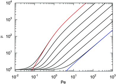 |
| | Fig. 1 Lagrangian multiplier μ = λ/λ0 [eqn (19)] as a function of Péclet number for the diffusion coefficient ratios Δ = DT/l2DR = 10−3, 3 × 10⁻³, 10−2, 3 × 10⁻², 10−1, 0.3, and 1 (left to right). The colored lines (left and right) correspond to the approximation of eqn (20) with the respective value of Δ. | |
The relaxation time is conveniently scaled by the friction coefficient γR. Hence,
| |  | (21) |
In the limit Pe = 0,
i.e.,
v0 = 0, this expression yields the Lagrangian multiplier
λ0 = 3/2
l2. Moreover, for
Δ = 0,
i.e., zero translational friction, we find
| |  | (22) |
This expression reduces to

in the limit Pe → ∞. Thus, the relaxation time

approaches zero for
v0 → ∞.
The dependence of the relaxation time on the Péclet number is presented in Fig. 2 for various ratios Δ. Since the activity dependence of τ is completely governed by the Lagrangian multiplier, the figure exhibits the same features as Fig. 1. In the asymptotic limit of large Péclet numbers, γRτ decreases as 1/Pe. For Pe < 1 and small Δ, there is an intermediate regime, where γRτ decreases as 1/Pe2 with increasing Pe. In the asymptotic limit Δ → 0, the functional dependence on Pe is captured by eqn (22).
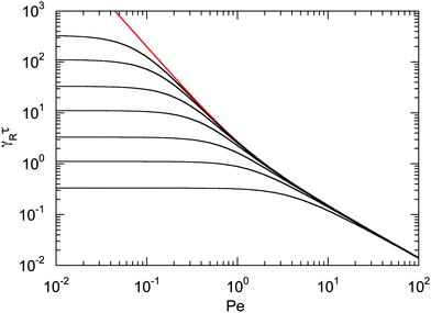 |
| | Fig. 2 Scaled dumbbell relaxation times γRτ [eqn (21)] as a function of Péclet number for the diffusion coefficient ratios Δ = DT/l2DR = 10−3, 3 × 10⁻³, 10−2, 3 × 10⁻², 10−1, 0.3, and 1 (top to bottom). The red line correspond to the approximation of eqn (22). | |
Fig. 1 and 2 reflect the tight coupling between the entropic degrees of freedom of a polymer, its finite extensibility, and activity, an aspect specific to polymers with their internal conformational degrees of freedom.
3.4 Bond vector autocorrelation function
The dynamics of the bond vector can be characterized by the correlation function| |  | (23) |
which is straightforwardly obtained as illustrated in Appendix A. In terms of the Péclet number (17), the correlation function reads| |  | (24) |
There are two exponentially decaying contributions to the correlation function, a contribution with the relaxation time τ, which strongly depends on the activity, and a contribution comprising γR, where the exponent is independent of self-propulsion. In the asymptotic limit Pe → ∞,  and the correlation function reduces to
| | | 〈R(t)·R(0)〉 = l2e−γRt. | (25) |
Here, the decay of the correlation function is independent of the propulsion force and solely governed by the orientational dynamics of the ABPs. This is similar to a rodlike active object propelled along its director, which changes by Brownian diffusion. In the previously addressed intermediate Pe regime, γRτ can be approximated by γRτ = 2/Pe2, which is much larger than unity for Pe < 1 (cf.Fig. 2), hence,| |  | (26) |
The correlation function decays with the relaxation time τ, which strongly depends on Pe (cf. remarks at the end of Section 3.3). In the limit Pe → 0, the relaxation behavior of a passive dumbbell is obtained.
In the exponentially decaying regimes, we can determine dumbbell-rotational diffusion coefficients DdR. With the definition  , eqn (25) and (26) imply
| | 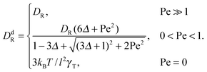 | (27) |
Hence, even for a moderate Péclet number, the rotational dynamics of the dumbbell is determined by the activity.
Fig. 3 provides an example of the bond vector correlation function. For the ratio of the diffusion coefficients, we choose Δ = 10−2, assuming that DR is larger than the thermal value. The correlation function decays exponentially in the limits Pe → ∞ and Pe → 0 according to eqn (25) and (26), respectively. The correlation functions decay in a non-exponential manner over a wide range of Péclet numbers including the considered values Pe = 0.5−5. Thereby, the decay is slower than exponential at short times. On longer time scales, the exponential decay is reached according to eqn (25) for Pe > 2 and eqn (26) for Pe < 2. In summary, the coupling of the internal polymer degrees of freedom and activity leads to a complex, in general, non-exponential decay of the bond vector correlation function.
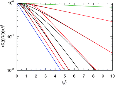 |
| | Fig. 3 Bond vector autocorrelation functions of a dumbbell as a function of the scaled time γRt for the Péclet numbers Pe = 0 (green), 0.5, 1.0, 1.5, 2.0, 3.0, 5.0, and ∞ (blue) (top to bottom). The diffusion coefficient ratio is set to Δ = 10−2. The red lines correspond to the two exponentially decaying terms of eqn (24). For Pe < 2, the long-time decay is determined by the decay of the first term on the right-hand side of eqn (24) (cf.eqn (26)), and for Pe > 2 by the second term (cf.eqn (25)). | |
4 Active dumbbell in shear flow
The nonequilibrium properties of passive Gaussian dumbbells in shear flow have been studied intensively. Various results are presented in ref. 79. Finite extensible Gaussian dumbbells, with the constraint of a constant mean square bond vector, have been studied in ref. 82. In particular, it has been shown that the finite extensibility of dumbbells and polymers is fundamental for shear thinning.79,82,85 In this section, an extension to active Brownian dumbbells under shear flow is provided.
4.1 Equation of motion
In shear flow with shear rate ![[small gamma, Greek, dot above]](https://www.rsc.org/images/entities/i_char_e0a2.gif) , the equations of motion eqn (11) become
, the equations of motion eqn (11) become| |  | (28) |
Flow is along the x-direction and the gradient is along the y-direction of the Cartesian reference frame. Here, the relaxation time τs = γT/4λskBT is introduced with the index ‘s’ to indicate the dependence of the relaxation time on the shear rate. Similarly, λs denotes the Lagrangian multiplier in the presence of shear flow. These are linear and independent equations as long as we assume the validity of eqn (5) and the correlation functions| |  | (29) |
in d dimensions. This implies the relation| |  | (30) |
i.e., independent velocity correlations for the Cartesian components, which does not necessarily apply to active systems with a velocity v = v0e, with the unit vector e. Here, the Cartesian components are coupled. However, we expect a minor (quantitative) difference between our approach, eqn (28) and (30), where 〈v2〉 = v02, and an approach applying the condition |v| = v0, as long as bond vectors are considered. Under this assumption, the solution of eqn (28) is| |  | (31) |
4.2 Lagrangian multiplier
The calculation of the mean square bond vector yields (cf. Appendix A)| |  | (32) |
As usual, we introduce the Weissenberg number85,96| | Wi = ![[small gamma, Greek, dot above]](https://www.rsc.org/images/entities/i_char_e0a2.gif) τ τ | (33) |
as a product of the shear rate and the relaxation time at a zero shear rate, which in our active system is τ of eqn (16). In addition, for the sake of brevity, we introduce the Lagrangian multiplier μs = λs/λ0 = τ0/τs. Hence, the constraint (2) turns into the condition for μs| | 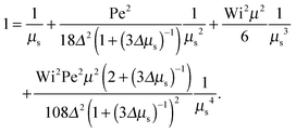 | (34) |
The Lagrangian multiplier μ is the solution of eqn (19) at zero shear.
Eqn (34) yields the following asymptotic dependencies:
• Passive dumbbell (Pe = 0, μ = 1)
| |  | (35) |
This is the expression derived in
ref. 82.
• Δ → 0 and Pe ≪ 1, or μsΔ ≪ 1
| |  | (36) |
Here, the same equation as for Pe = 0 is obtained,
i.e., we find the same dependence on the Weissenberg number as for the passive dumbbell. However, it has to be kept in mind that
μ = Pe
2/6
Δ in this limit. For Wi ≫ 1
| |  | (37) |
Hence, the Lagrangian multiplier depends quadratically on the Péclet number.
• Δ < 1, Pe < ∞, and Wi → ∞
| |  | (38) |
• Δ < 1, Pe ≫ 1, and Wi < ∞
| |  | (39) |
The solution of this equation is
| |  | (40) |
which yields in the asymptotic limit Wi → ∞
| |  | (41) |
i.e.,
μs depends linearly on the Péclet number. Note that
λs of an active dumbbell at large Péclet numbers exhibits a qualitative different dependence on the Weissenberg number as a passive dumbbell.
In eqn (36) and (40), the dependence on the Péclet number is solely via μ. As shown by the asymptotic expressions (37) and (41), we obtain a crossover from a Pe2 dependence for Pe ≪ 1 to a linear dependence for Pe ≫ 1.
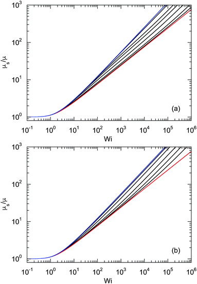
Fig. 4 shows Lagrangian-multiplier ratios μs/μ as a function of the Weissenberg number for Δ = 3 × 10⁻³ (a) and Δ = 0.3 (b) and various Péclet numbers. For the small diffusion coefficient ratio Δ = 3 × 10⁻³, we find a gradual change in the slope of μs/μ with increasing Pe. Starting from the curve of a passive dumbbell with the dependence μs ∼ Wi2/3 for Wi ≫ 1, the asymptotic dependence μs ∼ Wi1/2 is assumed for Pe → ∞. Thereby, the asymptotic dependence Wi2/3 for Wi → ∞ is essentially maintained for Wi > 103 and Pe < 0.1. Note, however, that for Pe ≳ 1 and Wi < ∞, there is a large range of Weissenberg numbers, where the Lagrangian multiplier exhibits the slope μs/μ ≈ 0.53 before the asymptotic dependence ∼Wi2/3 is assumed.
 |
| | Fig. 4 Ratios of Lagrange multipliers for active dumbbells under shear flow as a function of Weissenberg number for various Péclet numbers. The ratio of the diffusion coefficients is (a) Δ = 3 × 10⁻³ and (b) Δ = 3 × 10⁻¹. In (a), the Péclet numbers are Pe = 0 (blue), 10−1, 3 × 10⁻¹, 5 × 10⁻¹, 100, 3 × 100, 101, and ∞ (red) (left to right). The Péclet numbers in (b) are Pe = 0 (blue), 1, 3, 101, 3 × 101, 102, and ∞ (red) (left to right). | |
The changes of μs/μ with increasing Péclet number are qualitatively different for Δ = 0.3 compared to those for Δ = 3 × 10⁻³. For the large Δ value, we find a gradual change from the curve of a passive dumbbell to a curve which is described by eqn (40) and is dominated by activity. For small Δ, e.g., Δ = 3 × 10⁻³, however, we find first a gradual change of the slope to smaller values in the range 1 < Wi < 103 with increasing Pe < 0.1, and then, for Pe > 0.1, a “shift” of the whole curve to large Wi until the asymptotic behavior of eqn (40) is assumed.
4.3 Relaxation time
The nonequilibrium relaxation time τs follows viaeqn (33) from the Lagrangian multiplier μs. Hence, it is evident that τs strongly depends on the Péclet number. In terms of the friction coefficient γR, the equation for the scaled relaxation time γRτs is| | 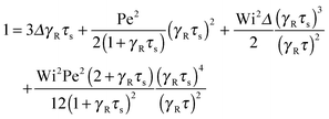 | (42) |
in analogy to that of the non-sheared dumbbell in Section 3.3.
The following asymptotic dependencies are obtained:
• Pe = 0 and Δ < 1
At zero Péclet number, μ = 1 and  . Combined with γR follows for Pe ≪ Δ
| |  | (43) |
• Δ → 0 and 0 < Pe ≪ 1
| |  | (44) |
• Δ<1 and Pe ≪ 1
With eqn (40)
| |  | (45) |
An example of the non-equilibrium relaxation times is provided in Fig. 5 for Δ = 3 × 10⁻³. As predicted, τs decreases with increasing Weissenberg number according to Wi−2/3 for Pe ≲ 0.2 and Wi−1/2 for Pe > 0.2. The strong influence of activity on the relaxation time is already visible for Pe ≳ 0.1 in the vicinity of Wi > 1. Here, and even more for larger Péclet numbers, the relaxation times exhibit the dependence τs ∼ Wi−1/2. However, the asymptotic dependence for Wi → ∞ is γRτs ∼ Wi−2/3 as long as Pe < ∞. In the limit Pe → 0, a Péclet number-independent asymptotic curve of a passive dumbbell is assumed already for Pe ≲ 10−2. This is a consequence of the fact that Δ is finite and hence μ is equal to unity. Taking the limit Δ → 0 first yields a different behavior, where γRτs ∼ Pe−2Wi2/3 over a broad range of Péclet numbers Pe ≪ 1. Hence, the relaxation time diverges with decreasing Pe. The asymptotic dependence of eqn (40) for Pe ≫ 1 is not yet reached for Pe = 10, as reflected by the small deviation between the analytical and numerically determined curve. The plateau values for Wi ≪ 1 follow from eqn (21)
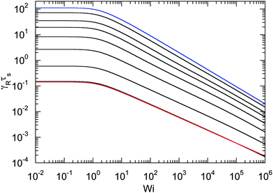 |
| | Fig. 5 Relaxation times γRτs as a function of Weissenberg number. The ratio of the diffusion coefficients is Δ = 3 × 10⁻³ and the Péclet numbers are Pe = 0 (blue), 10−1, 2 × 10⁻¹, 3 × 10⁻¹, 5 × 10⁻¹, 100, 3 × 100, and 101 (top to bottom). The curve for Pe = 0 (blue) corresponds to the solution of eqn (36) with μ = 1 (see also eqn (43)). The bottom curve (red) is calculated viaeqn (40). | |
4.4 Bond vector autocorrelation function
Straightforward calculations yield the bond-vector correlation functions for the Cartesian components (t ≥ 0) (cf. Appendix A)| | 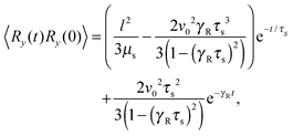 | (46) |
| | 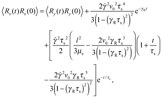 | (47) |
| | 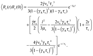 | (48) |
The bond-vector correlation function is then| | 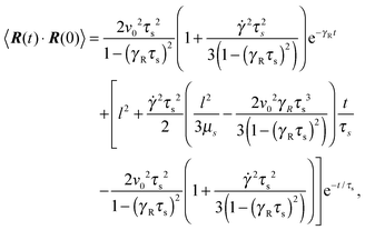 | (49) |
when we account for the constraint (2) and eqn (32). As for the non-sheared dumbbell, the correlation function is determined by two exponentially decaying contributions. The term including the relaxation time τs depends on both the Péclet number and the Weissenberg number. For γRτs ≪ 1, which follows for Pe ≫ 1 independent of the ratio Δ, the decay of the correlation function is determined by the first term on the right-hand side of eqn (49). Here, we find 〈R(t)·R(0)〉 ≈ l2e−γRt in the limit Wi ≫ 1. In the opposite limit, γRτs ≫ 1, both exponential terms contribute to the relaxation for moderate shear rates.
Fig. 6 displays examples of correlation functions for various diffusion coefficient ratios, Péclet numbers, and Weissenberg numbers. For an ABDB with a very large rotational diffusion coefficient, i.e., Δ ≪ 1 and small Pe values, both terms of eqn (49) contribute to the relaxation process. For Wi < 1, the relaxation is dominated by the second term of eqn (49) (e−t/τs) over several orders of magnitude of the correlation function. With increasing Wi, we observe a gradual crossover to the exponential decay l2e−γRt for Wi > 102. Note that even for smaller Weissenberg numbers, the long-time decay of the correlation function is given by e−γRt. For larger Péclet numbers at the same Δ, γRτs ≫ 1 and, hence, the decay of the correlation function is dominated by the first term on the right-hand side of eqn (49). The shear-rate dependent term in the brackets dominates at large Weissenberg numbers, however, the dependence  of the relaxation time renders the correlation function shear rate independent for these parameters.
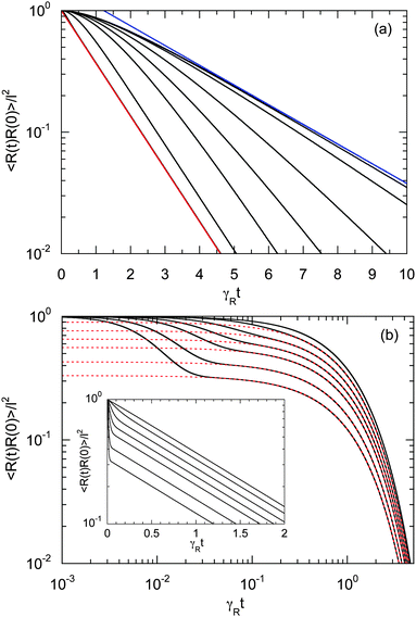 |
| | Fig. 6 Bond-vector autocorrelation functions of a dumbbell under shear flow as a function of the scaled time γRt for various Weissenberg numbers. (a) Correlations are displayed for Δ = 3 × 10⁻³, Pe = 1, and Wi = 0, 1, 2, 5, 10, 20, 100, and ∞ (red) (top to bottom). The blue line represents the exponential e−t/τs, and the red line e−γRt. (b) Correlations are shown for Δ = 3 × 10⁻¹, Pe = 10, and Wi = 0, 101, 4 × 101, 102, 2 × 10², 5 × 10² and 103 (top to bottom). The red dashed lines represent the exponential decay (e−γRt) of the first term on the right-hand side of eqn (49). The inset shows the same curves in a semi-log representation. | |
A smaller rotational diffusion coefficient yields a clear two-state decay of the correlation function, as shown in Fig. 6(b) for Δ = 0.3. In the limit γRt → 0, the term with the exponential decay e−t/τs dominates. Since γRτs < 1, this term decays faster than the term e−γRt. Thus, the latter term determines the long time behavior. This term is clearly shear rate dependent. Specifically for larger Weissenberg numbers, the “plateau” decreases with increasing Wi (cf.Fig. 6(b)). This is related to the fact that γτs ∼ Wi−κ with an exponent κ > 1/2, such that a dependence on the Weissenberg number remains, i.e., 〈R(t)·R(0)〉 ∼ Wi2−4κ. Note that aside from this relation, τs itself depends on the shear rate.
4.5 Shear-induced deformation
The correlation functions (46) and (47) yield the Cartesian components of the mean square bond vector under shear| |  | (50) |
| |  | (51) |
and 〈Rz2〉 = 〈Ry2〉. Evidently, the gradient component 〈Ry2〉 only depends on the shear rate via τs, whereas the flow component 〈Rx2〉 explicitly depends on ![[small gamma, Greek, dot above]](https://www.rsc.org/images/entities/i_char_e0a2.gif) additionally. In terms of the Péclet number, and taking into account the constraint (2), eqn (50) and (51) become
additionally. In terms of the Péclet number, and taking into account the constraint (2), eqn (50) and (51) become| |  | (52) |
These equations depend on the Weissenberg number only implicitly via μs. Most importantly, the constraint couples the various Cartesian components of the bond vector. At zero shear, the bond orientation is isotropic, hence 〈Rx2〉 = 〈Ry2〉 = 〈Rz2〉 = l2/3. Shear flow breaks the symmetry, and 〈Ry2〉 → 0 for Wi → ∞, since μs → ∞ in that limit as is evident from Fig. 4. As a consequence, 〈Rx2〉 → l2 for Wi → ∞, which indicates the alignment of the dumbbell along the flow direction.
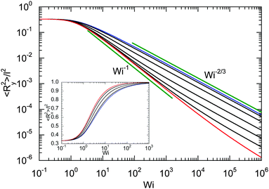
Fig. 7 provides an example of the dumbbell deformation for various Péclet numbers. For Pe = 0, eqn (50) and (51) reduce to those provided in ref. 82. Here, 〈Ry2〉 decreases as Wi−2/3 with increasing Weissenberg number. For large Péclet numbers the second term on the right-hand side of eqn (51) dominates, and the deformation transverse to the flow direction decreases as Wi−1 for moderate Pe. In the asymptotic limit Wi → ∞, 〈Ry2〉 decreases as Wi−2/3 with increasing Wi. As discussed in Section 4.2 in connection with the Lagrangian multiplier, a somewhat different dependence on the Weissenberg number can be observed, depending on the particular Péclet number.
 |
| | Fig. 7 Deformation transverse to the flow direction (gradient direction) of an ABDB as a function of shear rate for Δ = 0.3 and the Péclet numbers Pe = 0 (blue), 1, 3, 10, 30, 100, 500, and ∞ (red) (top to bottom). The straight lines indicate the power-law decay Wi−2/3 for Pe = 0 (top) and Wi−1 for Pe → ∞ (bottom). The inset displays the deformation along the flow direction for the Péclet numbers Pe = 0 (blue), 1, 3, 10, and ∞ (red) (right to left). | |
The inset of Fig. 7 displays the deformation along the flow direction. Starting from the equilibrium value l2/3, 〈Rx2〉 assumes the value l2 in the limit Wi → ∞, as required by the constraint (2). Thereby, the increase of 〈Rx2〉 depends on the Péclet number, and 〈Rx2〉 increases somewhat faster at larger Péclet numbers.
4.6 Shear-induced alignment
Shear flow implies a preferred alignment of the ABDB with respect to the flow direction, as is well known for passive polymers.82,84,96 This alignment is characterized by the angle χ between the bond vector R and the flow direction. The angle itself is obtained from the relation| |  | (54) |
Insertion of the correlations eqn (46)–(48) yields| |  | (55) |
where μ and μS are the solutions of eqn (19) and (34), respectively. For Pe = 0, eqn (55) reduces to the expression provided in ref. 82.
For Wi ≪ 1, μs = μ and tan(2χ) decreases as 1/Wi. The latter dependence would also apply for dumbbells/polymers with extensible bonds (Rouse/Zimm model), i.e., under shear flow the polymer-contour length could increase ad infinitum. In the case of the dumbbell, this nonphysical behavior is prevented by the constraint (2). As a consequence, the alignment of finite extensible passive dumbbells is given by tan(2χ) ∼ Wi−1/3 at large shear rates.82,84 Activity changes the large-Weissenberg-number behavior and leads to the dependence tan(2χ) ∼ Wi−1/2 as illustrated in Fig. 8.
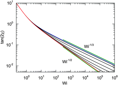 |
| | Fig. 8 Dependence of the shear-induced alignment of an ABDB [eqn (54)] on the shear rate for Δ = 0.3 and the Péclet numbers Pe = 0 (blue), 1, 3, 10, 30, 100, and ∞ (red) (top to bottom). The straight lines indicate the power-law decay Wi−1/3 for Pe = 0 (top) and Wi−1/2 for Pe → ∞ (bottom). | |
Alignment is tightly linked to the rheological properties of polymers and rodlike colloids,84,96 thus activity strongly affects the viscosity of a dilute solution of ABDBs.
4.7 Shear viscosity
The shear viscosity η of a dilute solution of ABDBs follows from the relation η = σxy/![[small gamma, Greek, dot above]](https://www.rsc.org/images/entities/i_char_e0a2.gif) , where σxy is the stress tensor. The stress tensor itself is calculated from its virial representation,58,82,83i.e.,
, where σxy is the stress tensor. The stress tensor itself is calculated from its virial representation,58,82,83i.e.,| |  | (56) |
for a single ABDB, with the volume V of the system and the forces defined in eqn (3). The “swimm” force γTvi does not provide a contribution to the shear stress,58 hence, the shear stress is solely determined by the bond forces. Evaluation of the averages yields the viscosity| |  | (57) |
which explicitly and via τs depends on the propulsion velocity. The shear rate dependence enters only via the relaxation time. The zero-shear viscosity η0 follows for Wi = 0, i.e., τs has to be replaced by τ of eqn (16).
The zero-shear viscosity itself depends on the Péclet number. For Pe = 0, η0 = kBTτ0/2, or, expressed in units of γR,
| |  | (58) |
In the asymptotic limit Pe → ∞,

, and hence,
η0(Pe = ∞) = 2
η0(Pe = 0),
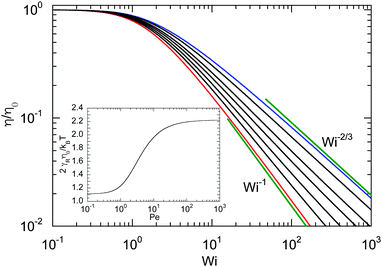
i.e., the viscosity at large Péclet numbers is twice as large as that at zero Pe. The explicit dependence of
η0 is presented in the inset of
Fig. 9. Activity evidently yields an increase of the zero shear viscosity.
 |
| | Fig. 9 Dependence of the shear viscosity of an ABDB on the shear rate for Δ = 0.3 and Pe = 0 (blue), 1, 2, 3, 5, 10, and ∞ (red) (top to bottom). The straight lines indicate the power-law decay Wi−2/3 for Pe = 0 (top) and Wi−1 for Pe → ∞ (bottom). Inset: Zero shear viscosity (Wi = 0) as a function of Péclet number. | |
The shear rate dependence of the viscosity is illustrated in Fig. 9. As expected, a dilute solution of ABDBs is shear thinning. Thereby, activity significantly affects the extent of shear thinning. For passive systems, the viscosity decreases asymptotically as Wi−2/3 at large shear rates. The slope changes gradually with increasing Péclet number, and η decreases as Wi−1 with increasing shear rate in the limit Pe → ∞. However, already for moderate Péclet numbers on the order of P ≈ 10, we observe a nearly linear decrease of η over a large range of shear rates.
5 Enthalpic dumbbell
As pointed out several times, the dumbbell harmonic bond (1) mimics the conformational properties of a polymer, i.e., its entropic degrees of freedom, and the constraint (2) accounts for the finite polymer extensibility. In the case of an enthalpic bond, i.e., a harmonic bond, where eqn (1) describes the stretching energy of the bond, no constraint exists and λ is connected to the spring constant K of the harmonic potential via λ = K/2kBT. An activity and shear independent spring constant changes the conformational, dynamical, and rheological properties of the dumbbell qualitatively. Specifically, the Lagrangian multipliers obey λ = λs = λ0, and thus, the relaxation times τ and τs are independent of activity and shear rate and are given by τ = τs = γT/2K. As a further consequence, μ = μs = 1.
For convenience, we list several of the important quantities of the enthalpic dumbbell.
(i) No shear flow
• Mean square bond vector
Without shear, eqn (15) is given by
| |  | (59) |
in terms of the Péclet number. Evidently, the mean square bond length is affected by the activity and 〈
R2〉 grows quadratically with Pe.
(ii) With shear flow
• Mean square bond vector transverse to the flow direction
Without constraint, the Cartesian components of any quantity are decoupled. Hence, the deformation along the gradient and vorticity directions of the mean square bond vector is independent of the shear flow and is given by 〈Ry2〉 = 〈Rz2〉 = 〈R2〉/3, with 〈R2〉 of eqn (59).
• Mean square bond vector along the flow direction
In the direction of flow, we find
| |  | (60) |
Thus, the deformation increases quadratically with the shear rate and the bond is stretched ad infinitum with increasing Wi.
• Alignment
The bond alignment [eqn (55)] is independent of activity and decreases with increasing Weissenberg number as tan(2χ) = 2/Wi.
• Viscosity
Since τs = τ is independent of the shear rate, the viscosity [eqn (57)] is independent of Wi. Thus, the harmonic enthalpic dumbbell shows no shear thinning behavior. However, the viscosity depends on activity and increases quadratically with increasing Péclet number.
In summary, finite polymer extensibility leads to a drastic qualitatively different nonequilibrium behavior.
6 Summary and conclusions
We have investigated the dynamical properties of an active Brownian dumbbell, both in the absence and the presence of shear flow. The dumbbell is comprised of two active Brownian particles, which are linked by a flexible bond. The finite extensibility of the bond is captured in a mean-field manner by a prescribed mean square bond length. The latter limitation strongly couples the entropic degrees of freedom with activity and the external field. The simple model allows us to find analytical solutions for the relaxation time and the bond-vector correlation function. Both quantities strongly depend on the Péclet number. Thereby, Péclet number regimes are obtained with distinctly different dependencies on Pe for small Δ = DT/l2DR, i.e., large rotational diffusion coefficients.
Activity strongly affects the dynamical properties of ABDBs in shear flow. Specifically, the shear rate dependence of the relaxation time is qualitatively different from that of a passive dumbbell; it changed for Wi > 1 from τs ∼ Wi−2/3 for Pe ≪ 1 to τs ∼ Wi−1/2 for Pe > 1. Since the relaxation time is essentially determining the tumbling time under flow,84 a weaker dependence of the tumbling time on the shear rate is obtained. In addition, ABDBs are better aligned with the flow, which results in a stronger shear thinning behavior and, hence, smaller viscosity at the same Weissenberg number.
In general, the obtained results highlight the effect of activity on the non-equilibrium dynamical properties of active systems with internal degrees of freedom. The dumbbell relaxation can be linked to the longest relaxation time of a polymer. Naturally, the many more internal degrees of freedom of flexible and semiflexible polymers give rise to an intricate dynamical behavior on the respective time scales, which are affected by activity. Nevertheless, we expect that the long-time behavior is captured by our dumbbell model. The dynamical aspects on shorter time scales, specifically for semiflexible polymers, remain to be elucidated. As is well known, the dynamics of long passive polymers in dilute solution is governed by hydrodynamic interactions.79,97–99 Such interactions are absorbed in the friction coefficient for dumbbells. However, hydrodynamic interactions are expected to be important for active polymers. This is another aspect, which deserves to be considered in detail.95
A Bond-length constraint and bond vector correlation functions
A.1 Bond length constraint
In the stationary state, the bond-length constraint (15) is given by| |  | (61) |
in terms of the solution (12) of the equation of motion (11). The correlation functions of the random variables Δv and ΔΓ follow as| | | 〈ΔΓ(t)·ΔΓ(t′)〉 = 12γTkBTδ(t − t′), | (62) |
| | | 〈Δν(t)·Δν(t′)〉 = 2v02e−γR|t − t′|. | (63) |
Insertion of these correlation functions leads to| |  | (64) |
Evaluation of the integrals yields eqn (15).
A.2 Bond vector correlation function: no shear
The bond vector correlation function (23) is obtained in a similar fashion. In terms of the solution (12) of the equations of motion, the correlation function reads| |  | (65) |
The calculation of the correlation functions of the random forces leads to| |  | (66) |
Evaluation of the integrals and insertion of eqn (2) yield eqn (23) and (24).
A.3 Bond vector correlation function: shear
Under shear, the bond vector correlation function along the shear direction is
Inserting the correlation functions of the random variables, the correlation function becomes
| |  | (67) |
Since the correlation functions along the gradient and vorticity directions are unaffected by shear flow, they are given by the respective Cartesian components of
eqn (66), hence
| |  | (68) |
The correlation function 〈
R(
t′)·
R(
t′′)〉 follows from
eqn (23) with the argument |
t′ −
t′′|,
i.e.,
t is replaced by |
t′ −
t′′|. Finally,
eqn (46)–(48) follow by integration.
Acknowledgements
Helpful discussions with Thomas Eisenstecken and the financial support of the project by the DFG within the priority program SPP 1726 “Microswimmers” are gratefully acknowledged.
References
- J. Elgeti, R. G. Winkler and G. Gompper, Rep. Prog. Phys., 2015, 78, 056601 CrossRef CAS PubMed.
- M. F. Copeland and D. B. Weibel, Soft Matter, 2009, 5, 1174 RSC.
- N. C. Darnton, L. Turner, S. Rojevsky and H. C. Berg, Biophys. J., 2010, 98, 2082 CrossRef CAS PubMed.
- D. B. Kearns, Nat. Rev. Microbiol., 2010, 8, 634–644 CrossRef CAS PubMed.
- K. Drescher, J. Dunkel, L. H. Cisneros, S. Ganguly and R. E. Goldstein, Proc. Natl. Acad. Sci. U. S. A., 2011, 10940, 108 Search PubMed.
- J. D. Partridge and R. M. Harshey, J. Bacteriol., 2013, 195, 909 CrossRef CAS PubMed.
- J. Bialké, T. Speck and H. Löwen, Phys. Rev. Lett., 2012, 108, 168301 CrossRef PubMed.
- I. Buttinoni, J. Bialké, F. Kümmel, H. Löwen, C. Bechinger and T. Speck, Phys. Rev. Lett., 2013, 110, 238301 CrossRef PubMed.
- B. M. Mognetti, A. Šarić, S. Angioletti-Uberti, A. Cacciuto, C. Valeriani and D. Frenkel, Phys. Rev. Lett., 2013, 111, 245702 CrossRef CAS PubMed.
- I. Theurkauff, C. Cottin-Bizonne, J. Palacci, C. Ybert and L. Bocquet, Phys. Rev. Lett., 2012, 108, 268303 CrossRef CAS PubMed.
- Y. Fily, S. Henkes and M. C. Marchetti, Soft Matter, 2014, 10, 2132 RSC.
- X. Yang, M. L. Manning and M. C. Marchetti, Soft Matter, 2014, 10, 6477 RSC.
- J. Stenhammar, D. Marenduzzo, R. J. Allen and M. E. Cates, Soft Matter, 2014, 10, 1489 RSC.
- Y. Fily, A. Baskaran and M. F. Hagan, Soft Matter, 2014, 10, 5609 RSC.
- G. S. Redner, M. F. Hagan and A. Baskaran, Phys. Rev. Lett., 2013, 110, 055701 CrossRef PubMed.
- Y. Fily and M. C. Marchetti, Phys. Rev. Lett., 2012, 108, 235702 CrossRef PubMed.
- R. Großmann, L. Schimansky-Geier and P. Romanczuk, New J. Phys., 2012, 14, 073033 CrossRef.
- V. Lobaskin and M. Romenskyy, Phys. Rev. E: Stat., Nonlinear, Soft Matter Phys., 2013, 87, 052135 CrossRef PubMed.
- A. Zöttl and H. Stark, Phys. Rev. Lett., 2014, 112, 118101 CrossRef PubMed.
- A. Wysocki, R. G. Winkler and G. Gompper, EPL, 2014, 105, 48004 CrossRef.
-
H. C. Berg, E. Coli in Motion, Springer, 2004 Search PubMed.
- S. Ramaswamy, Annu. Rev. Condens. Matter Phys., 2010, 1, 323 CrossRef.
- F. J. Nédélec, T. Surrey, A. C. Maggs and S. Leibler, Nature, 1997, 389, 305 CrossRef PubMed.
-
J. Howard, Mechanics of motor proteins and the cytoskeleton, Sinauer Associates Sunderland, MA, 2001 Search PubMed.
- K. Kruse, J. F. Joanny, F. Jülicher, J. Prost and K. Sekimoto, Phys. Rev. Lett., 2004, 92, 078101 CrossRef CAS PubMed.
- A. R. Bausch and K. Kroy, Nat. Phys., 2006, 2, 231 CrossRef CAS.
- F. Jülicher, K. Kruse, J. Prost and J.-F. Joanny, Phys. Rep., 2007, 449, 3 CrossRef.
- Y. Harada, A. Noguchi, A. Kishino and T. Yanagida, Nature, 1987, 326, 805 CrossRef CAS PubMed.
- V. Schaller, C. Weber, C. Semmrich, E. Frey and A. R. Bausch, Nature, 2010, 467, 73 CrossRef CAS PubMed.
- M. C. Marchetti, J. F. Joanny, S. Ramaswamy, T. B. Liverpool, J. Prost, M. Rao and R. A. Simha, Rev. Mod. Phys., 2013, 85, 1143 CrossRef CAS.
- J. Prost, F. Jülicher and J.-F. Joanny, Nat. Phys., 2015, 11, 111 CrossRef CAS.
- T. Vicsek and A. Zafeiris, Phys. Rep., 2012, 517, 71 CrossRef.
- J. R. Howse, R. A. L. Jones, A. J. Ryan, T. Gough, R. Vafabakhsh and R. Golestanian, Phys. Rev. Lett., 2007, 99, 048102 CrossRef PubMed.
- G. Volpe, I. Buttinoni, D. Vogt, H. J. Kümmerer and C. Bechinger, Soft Matter, 2011, 7, 8810 RSC.
- Y. Mei, A. A. Solovev, S. Sanchez and O. G. Schmidt, Chem. Soc. Rev., 2011, 40, 2109 RSC.
- B. ten Hagen, F. Kümmel, R. Wittkowski, D. Takagi, H. Löwen and C. Bechinger, Nat. Commun., 2014, 5, 4829 CrossRef CAS PubMed.
- B. Scharf, J. Bacteriol., 2002, 184, 5979 CrossRef CAS PubMed.
- A. Cordoba, J. D. Schieber and T. Indei, RSC Adv., 2014, 4, 17935 RSC.
- Y. Sumino, K. H. Nagai, Y. Shitaka, D. Tanaka, K. Yoshikawa, H. Chate and K. Oiwa, Nature, 2012, 483, 448 CrossRef CAS PubMed.
-
S. Kim and S. J. Karrila, Microhydrodynamics: principles and selected applications, Butterworth-Heinemann, Boston, 1991 Search PubMed.
- E. Lauga and T. R. Powers, Rep. Prog. Phys., 2009, 72, 096601 CrossRef.
- K. Drescher, R. E. Goldstein, N. Michel, M. Polin and I. Tuval, Phys. Rev. Lett., 2010, 105, 168101 CrossRef PubMed.
- J. S. Guasto, K. A. Johnson and J. P. Gollub, Phys. Rev. Lett., 2010, 105, 168102 CrossRef PubMed.
- N. Watari and R. G. Larson, Biophys. J., 2010, 98, 12 CrossRef CAS PubMed.
- J. Hu, M. Yang, G. Gompper and R. G. Winkler, Soft Matter, 2015, 11, 7843 RSC.
- S. Ghose and R. Adhikari, Phys. Rev. Lett., 2014, 112, 118102 CrossRef PubMed.
- G. S. Klindt and B. M. Friedrich, Phys. Rev. E: Stat., Nonlinear, Soft Matter Phys., 2015, 92, 063019 CrossRef PubMed.
- F. Peruani, L. Schimansky-Geier and M. Bär, Eur. Phys. J.: Spec. Top., 2010, 191, 173 CrossRef.
- P. Romanczuk, M. Bär, W. Ebeling, B. Lindner and L. Schimansky-Geier, Eur. Phys. J.: Spec. Top., 2012, 202, 1 CrossRef CAS.
- M. Yang and M. Ripoll, Soft Matter, 2014, 10, 1006 RSC.
- A. P. Solon, J. Stenhammar, R. Wittkowski, M. Kardar, Y. Kafri, M. E. Cates and J. Tailleur, Phys. Rev. Lett., 2015, 114, 198301 CrossRef PubMed.
- A. P. Solon, Y. Fily, A. Baskaran, M. E. Cates, Y. Kafri, M. Kardar and J. Tailleur, Nat. Phys., 2015, 11, 673 CrossRef CAS.
- S. C. Takatori, W. Yan and J. F. Brady, Phys. Rev. Lett., 2014, 113, 028103 CrossRef CAS PubMed.
- C. Maggi, U. M. B. Marconi, N. Gnan and R. Di Leonardo, Sci. Rep., 2015, 5, 10742 CrossRef PubMed.
- F. Ginot, I. Theurkauff, D. Levis, C. Ybert, L. Bocquet, L. Berthier and C. Cottin-Bizonne, Phys. Rev. X, 2015, 5, 011004 Search PubMed.
- E. Bertin, Physics, 2015, 8, 44 CrossRef.
- T. Speck, A. M. Menzel, J. Bialké and H. Löwen, J. Chem. Phys., 2015, 142, 224109 CrossRef PubMed.
- R. G. Winkler, A. Wysocki and G. Gompper, Soft Matter, 2015, 11, 6680 RSC.
- T. Vicsek, A. Czirók, E. Ben-Jacob, I. Cohen and O. Shochet, Phys. Rev. Lett., 1995, 75, 1226 CrossRef CAS PubMed.
- H. H. Wensink and H. Löwen, Phys. Rev. E: Stat., Nonlinear, Soft Matter Phys., 2008, 78, 031409 CrossRef CAS PubMed.
- Y. Yang, V. Marceau and G. Gompper, Phys. Rev. E: Stat., Nonlinear, Soft Matter Phys., 2010, 82, 031904 CrossRef PubMed.
- M. Abkenar, K. Marx, T. Auth and G. Gompper, Phys. Rev. E: Stat., Nonlinear, Soft Matter Phys., 2013, 88, 062314 CrossRef PubMed.
- D. Loi, S. Mossa and L. F. Cugliandolo, Soft Matter, 2011, 7, 10193 RSC.
- A. Ghosh and N. S. Gov, Biophys. J., 2014, 107, 1065 CrossRef CAS PubMed.
- R. E. Isele-Holder, J. Elgeti and G. Gompper, Soft Matter, 2015, 11, 7181 RSC.
- T. B. Liverpool, A. C. Maggs and A. Ajdari, Phys. Rev. Lett., 2001, 86, 4171 CrossRef CAS PubMed.
- D. Sarkar, S. Thakur, Y.-G. Tao and R. Kapral, Soft Matter, 2014, 10, 9577 RSC.
- R. Chelakkot, A. Gopinath, L. Mahadevan and M. F. Hagan, J. R. Soc., Interface, 2013, 11, 20130884 CrossRef PubMed.
- G. Jayaraman, S. Ramachandran, S. Ghose, A. Laskar, M. S. Bhamla, P. B. S. Kumar and R. Adhikari, Phys. Rev. Lett., 2012, 109, 158302 CrossRef PubMed.
- A. Laskar, R. Singh, S. Ghose, G. Jayaraman, P. B. S. Kumar and R. Adhikari, Sci. Rep., 2013, 3, 1964 Search PubMed.
- H. Jiang and Z. Hou, Soft Matter, 2014, 10, 1012 RSC.
- J. P. Hernandez-Ortiz, C. G. Stoltz and M. D. Graham, Phys. Rev. Lett., 2005, 95, 204501 CrossRef PubMed.
- V. B. Putz, J. Dunkel and J. M. Yeomans, Chem. Phys., 2010, 375, 557 CrossRef CAS.
- A. Furukawa, D. Marenduzzo and M. E. Cates, Phys. Rev. E: Stat., Nonlinear, Soft Matter Phys., 2014, 90, 022303 CrossRef PubMed.
- C. Valeriani, M. Li, J. Novosel, J. Arlt and D. Marenduzzo, Soft Matter, 2011, 7, 5228 RSC.
- A. Suma, G. Gonnella, D. Marenduzzo and E. Orlandini, EPL, 2014, 108, 56004 CrossRef.
- L. F. Cugliandolo, G. Gonnella and A. Suma, Phys. Rev. E: Stat., Nonlinear, Soft Matter Phys., 2015, 91, 062124 CrossRef PubMed.
- A. Suma, G. Gonnella, G. Laghezza, A. Lamura, A. Mossa and L. F. Cugliandolo, Phys. Rev. E: Stat., Nonlinear, Soft Matter Phys., 2014, 90, 052130 CrossRef PubMed.
-
R. B. Bird, C. F. Curtiss, R. C. Armstrong and O. Hassager, Dynamics of Polymer Liquids, John Wiley & Sons, New York, 1987, vol. 2 Search PubMed.
- A. Puliafito and K. Turitsyn, Phys. D, 2005, 211, 9 CrossRef CAS.
- Y.-G. Tao, I. O. Götze and G. Gompper, J. Chem. Phys., 2008, 128, 144902 CrossRef PubMed.
- B. Kowalik and R. G. Winkler, J. Chem. Phys., 2013, 138, 104903 CrossRef PubMed.
- R. G. Winkler and P. Reineker, Macromolecules, 1992, 25, 6891 CrossRef CAS.
- R. G. Winkler, Soft Matter, 2010, 6, 6183 RSC.
- R. G. Winkler, J. Chem. Phys., 2010, 133, 164905 CrossRef PubMed.
- M. G. Bawendi and K. F. Freed, J. Chem. Phys., 1985, 83, 2491 CrossRef CAS.
- R. A. Harris and J. E. Hearst, J. Chem. Phys., 1966, 44, 2595 CrossRef CAS.
- W. Carl, Macromol. Theory Simul., 1996, 5, 1 CrossRef CAS.
- F. Ganazzoli, G. Allegra, E. Colombo and M. D. Vitis, Macromolecules, 1995, 28, 1076 CrossRef CAS.
- M. Dolgushev, T. Guérin, A. Blumen, O. Bénichou and R. Voituriez, J. Chem. Phys., 2014, 141, 014901 CrossRef PubMed.
- J. Saragosti, P. Silberzan and A. Buguin, PLoS One, 2012, 7, e35412 CAS.
- S. Tavaddod, M. A. Charsooghi, F. Abdi, H. R. Khalesifard and R. Golestanian, Eur. Phys. J. E: Soft Matter Biol. Phys., 2011, 34, 1 CrossRef CAS PubMed.
-
H. Risken, The Fokker-Planck Equation, Springer, Berlin, 1989 Search PubMed.
- P. Hänggi and P. Jung, Adv. Chem. Phys., 1995, 89, 239 CrossRef.
- A. Kaiser, S. Babel, B. ten Hagen, C. von Ferber and H. Löwen, J. Chem. Phys., 2015, 142, 124905 CrossRef PubMed.
- C.-C. Huang, R. G. Winkler, G. Sutmann and G. Gompper, Macromolecules, 2010, 43, 10107 CrossRef CAS.
-
M. Doi and S. F. Edwards, The Theory of Polymer Dynamics, Clarendon Press, Oxford, 1986 Search PubMed.
- L. Harnau, R. G. Winkler and P. Reineker, J. Chem. Phys., 1996, 104, 6355 CrossRef CAS.
- E. P. Petrov, T. Ohrt, R. G. Winkler and P. Schwille, Phys. Rev. Lett., 2006, 97, 258101 CrossRef CAS PubMed.
|
| This journal is © The Royal Society of Chemistry 2016 |
Click here to see how this site uses Cookies. View our privacy policy here.  Open Access Article


 . Evidently, the bond force increases with increasing rotational diffusion coefficient and increasing Péclet number. Without propulsion (Pe = 0), eqn (19) yields μ = 1.


 in the limit Pe → ∞. Thus, the relaxation time
  approaches zero for v0 → ∞.


 and the correlation function reduces to
 , eqn (25) and (26) imply

![[small gamma, Greek, dot above]](https://www.rsc.org/images/entities/i_char_e0a2.gif) , the equations of motion eqn (11) become
, the equations of motion eqn (11) become


![[small gamma, Greek, dot above]](https://www.rsc.org/images/entities/i_char_e0a2.gif) τ
τ


 . Combined with γR follows for Pe ≪ Δ


 of the relaxation time renders the correlation function shear rate independent for these parameters.


![[small gamma, Greek, dot above]](https://www.rsc.org/images/entities/i_char_e0a2.gif) additionally. In terms of the Péclet number, and taking into account the constraint (2), eqn (50) and (51) become
additionally. In terms of the Péclet number, and taking into account the constraint (2), eqn (50) and (51) become


![[small gamma, Greek, dot above]](https://www.rsc.org/images/entities/i_char_e0a2.gif) , where σxy is the stress tensor. The stress tensor itself is calculated from its virial representation,58,82,83i.e.,
, where σxy is the stress tensor. The stress tensor itself is calculated from its virial representation,58,82,83i.e.,


 , and hence, η0(Pe = ∞) = 2η0(Pe = 0), i.e., the viscosity at large Péclet numbers is twice as large as that at zero Pe. The explicit dependence of η0 is presented in the inset of Fig. 9. Activity evidently yields an increase of the zero shear viscosity.


