
 Open Access Article
 This Open Access Article is licensed under a
 Creative Commons Attribution 3.0 Unported Licence
Coarse-grained treatment of the self-assembly of colloids suspended in a nematic host phase
Sergej
Püschel-Schlotthauer
a,
Tillmann
Stieger
a,
Michael
Melle
a,
Marco G.
Mazza
b and
Martin
Schoen
ac
aStranski-Laboratorium für Physikalische und Theoretische Chemie, Fakultät für Mathematik und Naturwissenschaften, Technische Universität Berlin, Straße des 17. Juni 135, 10623 Berlin, Germany
bMax-Planck-Institut für Dynamik und Selbstorganisation, Am Faßberg 17, 37077 Göttingen, Germany
cDepartment of Chemical and Biomolecular Engineering, North Carolina State University, Engineering Building I, Box 7905, 911 Partners Way, Raleigh, NC 27695, USA
First published on 13th October 2015
Abstract
The complex interplay of molecular scale effects, nonlinearities in the orientational field and long-range elastic forces makes liquid-crystal physics very challenging. A consistent way to extract information from the microscopic, molecular scale up to the meso- and macroscopic scale is still missing. Here, we develop a hybrid procedure that bridges this gap by combining extensive Monte Carlo (MC) simulations, a local Landau–de Gennes theory, classical density functional theory, and finite-size scaling theory. As a test case to demonstrate the power and validity of our novel approach we study the effective interaction among colloids with Boojum defect topology immersed in a nematic liquid crystal. In particular, at sufficiently small separations colloids attract each other if the angle between their center-of-mass distance vector and the far-field nematic director is about 30°. Using the effective potential in coarse-grained two-dimensional MC simulations we show that self-assembled structures formed by the colloids are in excellent agreement with experimental data.
1 Introduction
Liquid crystals are fluids made of molecules that lack spherical symmetry. Instead, their molecules contain elongated, rigid cores that form nematic liquid crystals, or disk-like cores that produce discotic liquid crystals or even more complex shapes. This simple property of anisotropy produces a myriad consequences for the optical, mechanical and thermodynamic properties of liquid crystals. For example, as the temperature is decreased they undergo a series of phase transitions where the symmetry of their state is spontaneously broken. Starting from a high temperature isotropic fluid, where all orientations are equivalent, to a nematic state where orientational order is broken, to a smectic phase, where positional order is broken in one dimension.The molecular anisotropy produces effects on a macroscopic scale. In the nematic state, all molecules tend to align in the same direction, called the fluid's director.1 But any localized deviation of molecular orientations from the director will cause a restoring, elastic force. However, a single global orientation cannot be satisfied for all boundary conditions. A colloid immersed in the nematic fluid causes a specific preferential alignment of the liquid crystal molecules on its surface, which is termed anchoring. A spherical colloid has a symmetry incompatible with a global nematic director. Thus, defects in the orientational field will arise. These topological defects are points or lines that minimize the free energy of the liquid crystal subject to complex boundary conditions. Depending on details of the fluid and the anchoring of its molecules at the colloid, the orientational field can be of such dazzling complexity that experts are just beginning to unravel its structural details.2
If multiple colloids are immersed in a nematic liquid crystal, the distortions of the local director field also give rise to effective interactions between the colloids mediated by the nematic host fluid.3 These interactions may be used to self-assemble the colloids into supramolecular entities in a controlled (i.e., directed) manner. In this way ordered assemblies of colloids of an enormously rich structure with a great variety of symmetries may be built that would not otherwise exist without the ordered nature of the host phase.4,5 These self-assembled colloidal structures are also of practical importance, as they can be used to produce photonic crystals.6,7
The forces guiding colloidal self-assembly result from a complex interplay of molecular scale ordering, mesoscopic elastic interactions, and large scale topological arguments. While the framework of the Landau–de Gennes theory is appropriate for mesoscale effects, the elastic Frank–Oseen free energy is appropriate for long-range interactions.8 However, there is a gap between the microscopic, molecular information and the coarse-grained approaches used at the meso and macroscopic scale. No consistent method exists to transfer physical information from the molecular scale up to the scale where elastic forces and nonlinearities in the nematic interactions occur. Here, we pursue the goal of bridging this gap. The task is not idle, as there are physical situations that have so far eluded a precise explanation at the molecular level. As a test case to demonstrate power and validity of a novel hybrid approach developed in this work we take on the problem of colloidal self-assembly. Poulin and Weitz9 found experimentally that in a nematic phase the colloidal center-to-center distance vector r12 forms a “magic” angle of θ ≈ 30° with the global director ![[n with combining circumflex]](https://www.rsc.org/images/entities/b_i_char_006e_0302.gif) 0 if the liquid crystal molecules (mesogens) favor a local planar anchoring at the colloid's surface.10
0 if the liquid crystal molecules (mesogens) favor a local planar anchoring at the colloid's surface.10
Near an isolated colloid with planar anchoring the mesogens will produce a Boojum defect. While for such a single topological defect long-range approximation analogous to electrostatics can be sufficient, the complex interaction of multiple Boojum defects requires a more careful analysis. In previous theoretical attempts a much larger angle of about 50° is usually found.9,11 This number is based upon calculations where one employs the electrostatic analog of the Boojum defect topology.9 In fact, as stated explicitly by Poulin and Weitz “This theoretical value is different from the experimentally observed value for θ … since the theory is a long-range description that does not account for short-range effects”.9
Theoretical results similar to the experimental ones by Poulin and Weitz9 were recently found by Tasinkevych et al. through a direct minimization of a Landau–de Gennes free-energy functional.8 These authors demonstrate that the radial component of the elastic force has an attractive minimum around θ ≈ 30° for certain r12 = |r12|; this minimum shifts to larger θ as r12 increases. However, to date and to the best of our knowledge no molecular-scale work exists supporting the result of Tasinkevych et al.8 or the experimental findings by Poulin and Weitz.9
Another motivation for our work is the more recent experimental observation that between a pair of colloids in a nematic host repulsive and attractive forces act depending on θ.11 For example, at θ ≈ 30° the colloids attract each other whereas at θ = 0° and 90° repulsion between the colloids is observed.
To study these effects starting from a molecular-level based description we employ a combination of Monte Carlo (MC) simulations in the isothermal–isobaric and canonical ensembles, two-dimensional (2D), coarse-grained MC simulations in the canonical ensemble, classical density functional theory (DFT), concepts of finite-size scaling (FSS), and Landau–de Gennes (LdG) theory to investigate the effective interaction between a pair of spherical, chemically homogeneous colloids mediated by a nematic host phase.
The remainder of this manuscript is organized as follows. We begin in Section 2 with an introduction of our model system and its various constituents. Relevant theoretical concepts are introduced in Section 3. In Section 4 we present results of this study which we summarize and discuss in the closing Section 5 of this manuscript.
2 Model
In this work we consider the self-assembly of colloidal particles in two and three dimensions. The colloids are immersed in a nematic liquid-crystalline host fluid where an external field is invoked to control the global director0. The following three sections are devoted to introducing the various constituents of our model and to specifying their interactions with one another.
2.1 Host phase
The liquid crystal host phase is composed of N mesogens interacting with each other in a pairwise additive fashion. The interaction potential can be cast as| φmm(rij, ωi, ωj) = φiso(rij) + φanis(rij, ωi, ωj) | (1) |
For the isotropic contribution we adopt the well-known Lennard-Jones potential
 | (2) |
To derive an expression for the anisotropic contribution in eqn (1) we follow Giura and Schoen.12 From a lengthy but relatively straightforward derivation these authors show that
φanis(rij, ωi, ωj) = φatt(rij)Ψ(![[r with combining circumflex]](https://www.rsc.org/images/entities/b_i_char_0072_0302.gif) ij, ωi, ωj) ij, ωi, ωj) | (3) |
| Ψ(ij, ωi, ωj) = 5ε1P2[û(ωi)·û(ωj)] + 5ε2{P2[û(ωi)·ij] + P2[û(ωj)·ij]} | (4) |
ij = rij/rij are unit vectors specifying the orientation of mesogens i and j and the orientation of the center-of-mass distance vector, respectively, both in a space-fixed frame of reference. In addition, P2(x) = ½(3x2 − 1) is the second Legendre polynomial and the (dimensionless) anisotropy parameters 2ε1 = −ε2 = −0.08 are fixed throughout this work. Notice also that the first term on the right-hand side of eqn (4) matches the orientation dependence of interactions in the Maier–Saupe model13,14 whereas the next two terms account for the anisotropy of mesogen–mesogen attractions with enhanced sophistication.
2.2 External field
For a suitable choice of thermodynamic state parameters the host phase introduced in Section 2.1 exhibits isotropic and nematic phases.12 Unfortunately, when a nematic phase is forming in the bulk it is impossible to determine beforehand the direction of0. In fact, there is an infinite number of easy axes15 with which 0 may align in the bulk nematic phase.
To predict and control 0 it has therefore become customary to place the liquid crystal between solid substrates with specially prepared surfaces that tend to align mesogens in their vicinity in a desired way.16 Because orientational order in a nematic liquid crystal is a long-range phenomenon, substrate-induced alignment of mesogens allows one to control 0 on a length scale exceeding by far a molecular one. A host of different techniques to achieve a particular substrate anchoring of mesogens experimentally has been known for quite some time.17
In this work we take the substrates to be planar and structureless such that their surfaces are separated by a distance sz along the z-axis. Thus, the interaction between a mesogen and the substrates can be cast as
 | (5) |
The value of εms is chosen for two reasons. First, it guarantees a sufficiently strong alignment of mesogens with the surface so that fluctuation of 0 over the course of the simulations are negligible. Second, εms is still small enough to prevent from freezing those portions of the host phase that are located in the vicinity of the substrates.
The orientation dependence of the external field in our model enters through the anchoring function
| g(ωi) = [û(ωi)·êx]2 | (6) |
0 to the x-axis on average where |0·êx| ≃ 1 due to thermal fluctuations.
2.3 Colloidal particles
In addition, colloidal particles are immersed into the nematic liquid crystal. These colloids are spherical in shape, where r0 = 3.00σ is their hard-core radius, and have a chemically homogeneous surface. Similar to the planar substrates we envision the surfaces of the colloids to have been treated such that mesogens have a specific orientation with respect to the local surface normal of a colloid. Following earlier work by some of us18 we take the mesogen–colloid interaction potential to be given by | (7) |
In eqn (7), η is the inverse Debye screening length and parameters a1 and a2 have been introduced to guarantee that the minimum of φmc remains at a distance r0 + σ from the colloid's center of mass and to maintain the depth of the attractive well at εmc irrespective of η.18 Throughout this work we fix ησ = 0.50.
Last but not least, we introduce another anchoring function in eqn (7) which we take to be given by
| gc(cij, ωi) = [1 − |cij·û(ωi)|]2 | (8) |
cij = rcij/rcij is the local surface normal of the colloid. Hence, the anchoring function introduced in eqn (8) serves to align mesogens in a degenerate,15 locally planar fashion with respect to the colloid's surface.
3 Theory
To eventually simulate the self-assembly of several colloidal particles in a coarse-grained fashion we seek to represent the nematic host phase through an effective interaction potential. Key to this approach (as in all coarse-grained treatments) is a sensible protocol to integrate out irrelevant degrees of freedom while preserving the correct physics. Here, we seek to link a molecular-level description of the nematic host to a continuum treatment.3.1 Continuum approach
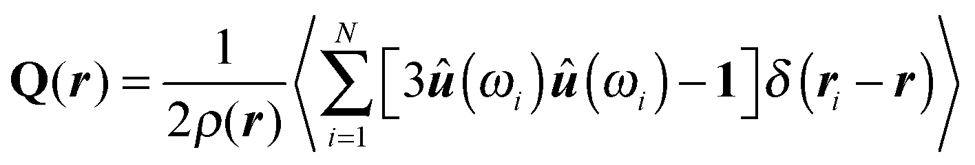
As already pointed out in Section 1, the presence of a colloid in a nematic liquid crystal causes(r) to deviate from 0 in certain regions near the colloid's surface. Associated with this distortion of (r) is a local deviation between the nematic order parameter and its bulk value in the absence of any colloid. Both, the distortion of (r) and the associated decline of S(r) cause changes in the free energy of the composite system (i.e., colloid plus nematic host). Adopting a continuum perspective a key quantity is the local alignment tensor Q(r) whose components can be cast as | (9) |
(r), and δαβ is the Kronecker symbol. The assumption underlying eqn (9) is that a spatial variation of the degree of nematic order of uniaxial symmetry and a deformation of the nematic director field are coupled (see also Section 4.4).
Therefore, the total change in free-energy density may readily be expressed as
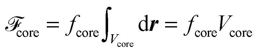
| Δf(r) = ΔfLdG(r) + fel(r) + fcore | (10) |
 | (11) |
![[/]](https://www.rsc.org/images/entities/char_e0ee.gif) S and QαβQβγQγα = ¾S3 This allows us to rewrite eqn (11) as
S and QαβQβγQγα = ¾S3 This allows us to rewrite eqn (11) as | (12) |
In eqn (11) as well as in eqn (12)
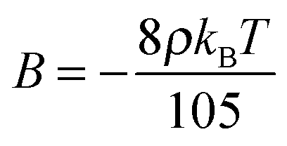
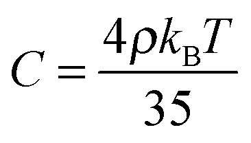
| Δf0 = ASb2 + BSb3 + CSb4 | (13) |
Next, the elastic contribution to Δf in the one-constant approximation (see below) may be cast as
 | (14) |
 | (15) |
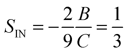
(r) occur on a length scale that is large compared to a molecular one. As we shall demonstrate below this is true in our system almost everywhere except inside the core of defects. To avoid an improper calculation of fFO(r) we restrict the evaluation of eqn (14) to regions outside the defect core.19–21 The latter is defined through the inequality S(r) ≤ SIN where SIN is the nematic order parameter at the IN phase transition in the host phase (and in the absence of any colloidal particle; see below).
Because we are restricting the use of eqn (14) by “cutting out” the defect core some correction to Δf due to the core region is required. As pointed out by de las Heras et al. it is necessary to include such a correction to the change in free-energy density because of the nanoscopic size of our colloidal particle.22 This correction, represented by fcore in eqn (10), will be discussed in some detail in Section 4.3.
Last but not least, we emphasize that within the framework of the present continuum theory the standard approach is to minimize the functional23
 | (16) |
(r) do not necessarily correspond to the global minimum of Δ![[scr F, script letter F]](https://www.rsc.org/images/entities/char_e141.gif) . This is in particular so if the structure of S(r) and (r) in thermodynamic equilibrium is rather complex.24 Second, there is no way within the framework of the continuum approach to determine the material constants A, B, C, and K (or L). Here one usually resorts to experimental information which is available for a few liquid crystals.25
. This is in particular so if the structure of S(r) and (r) in thermodynamic equilibrium is rather complex.24 Second, there is no way within the framework of the continuum approach to determine the material constants A, B, C, and K (or L). Here one usually resorts to experimental information which is available for a few liquid crystals.25
In closing, we emphasize that the expressions given in eqn (12) and (14) correspond to the same ground state. For example, in the absence of any perturbation, that is if S(r) = Sb and (r) = 0, ΔfLdG = fel = 0.
3.2 Molecular approach
(r) for a thermodynamic equilibrium situation via suitably defined ensemble averages. One may then feed S(r) and (r) into expressions such as eqn (12) and (14) to eventually obtain the absolute minimum of Δ [after an integration of Δf(r) over volume, see also Section 4.3].
Thus, to eventually compute Δ we begin by introducing the local alignment tensor
 | (17) |
(r).
However, to compute ΔfLdG(r) and fel(r) the material constants A, B, C, and K are required. Whereas this is relatively straightforward within the framework of MC simulations as far as K is concerned, one encounters serious difficulties to compute A, B, and C reliably. We address these difficulties below.
For the calculation of K we employ a method suggested by Allen and Frenkel.28,29 In their approach one considers fluctuations of Fourier components ![[Q with combining tilde]](https://www.rsc.org/images/entities/b_char_0051_0303.gif) (k) of Q(r). In the limit of |k| → 0 simple linear relationships exist from which the Frank constants K1, K2, and K3 associated with bend, twist, and splay deformations of (r) can be estimated reliably. Stieger et al.30 have recently applied the method of Allen and Frenkel28,29 to show that for the present model of the host phase K1 ≃ K2 ≃ K3 = K so that the one-constant form1 of fel in eqn (14) is an excellent approximation. Under the thermodynamic conditions used here (see Section 4.1), K ≃ 1.66εmmσ−1 is obtained.
(k) of Q(r). In the limit of |k| → 0 simple linear relationships exist from which the Frank constants K1, K2, and K3 associated with bend, twist, and splay deformations of (r) can be estimated reliably. Stieger et al.30 have recently applied the method of Allen and Frenkel28,29 to show that for the present model of the host phase K1 ≃ K2 ≃ K3 = K so that the one-constant form1 of fel in eqn (14) is an excellent approximation. Under the thermodynamic conditions used here (see Section 4.1), K ≃ 1.66εmmσ−1 is obtained.
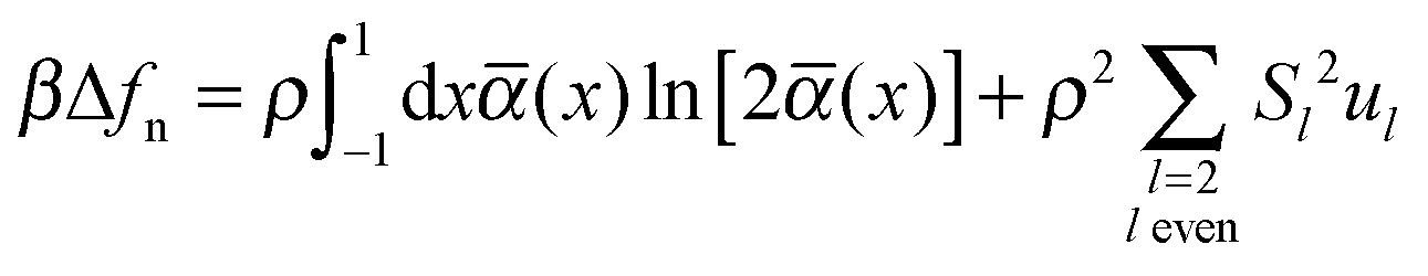
We therefore resort to a different approach based upon classical mean-field DFT. As demonstrated elsewhere32 the change in free energy–density of the bulk nematic relative to the isotropic phase can be cast as
 | (18) |
![[thin space (1/6-em)]](https://www.rsc.org/images/entities/char_2009.gif) θ, and θ is the azimuthal angle if we take the z-axis of our coordinate system to coincide with 0. Members of the set {Sl} defined on the interval [0, 1] are order parameters and {ul} are parameters that account for the contribution of anisotropic mesogen–mesogen interactions to the free energy, respectively.32
θ, and θ is the azimuthal angle if we take the z-axis of our coordinate system to coincide with 0. Members of the set {Sl} defined on the interval [0, 1] are order parameters and {ul} are parameters that account for the contribution of anisotropic mesogen–mesogen interactions to the free energy, respectively.32
The integrand on the right-hand side of eqn (18) contains the orientation distribution function ![[small alpha, Greek, macron]](https://www.rsc.org/images/entities/i_char_e0c2.gif) (x). It depends only on θ due to the uniaxial symmetry of the nematic phase and is normalized according to
(x). It depends only on θ due to the uniaxial symmetry of the nematic phase and is normalized according to
 | (19) |
(x) = ½. Again, because of the uniaxiality of the nematic phase we expand (x) in terms of Legendre polynomials {Pl} via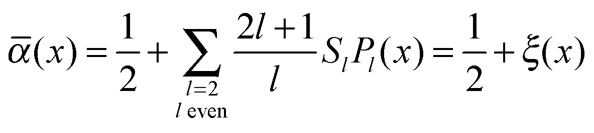 | (20) |
![[scr O, script letter O]](https://www.rsc.org/images/entities/char_e52e.gif) (ξ4) allows us to recast eqn (18) as
(ξ4) allows us to recast eqn (18) as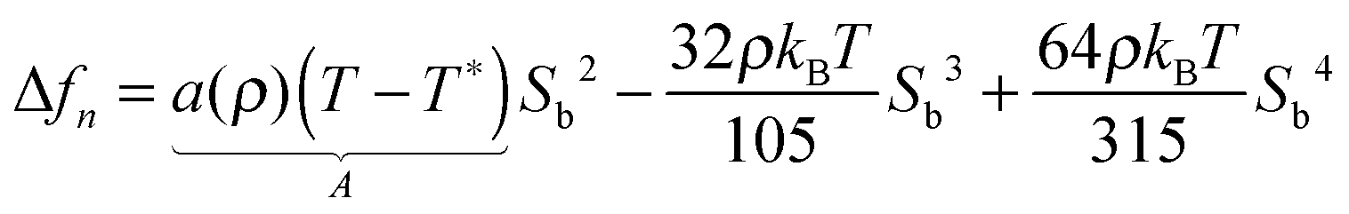 | (21) |
 | (22a) |
 | (22b) |
Unfortunately, at SMF level T* turns out to be grossly underestimated whereas at MMF level its value is equally grossly overestimated as a previous FSS study of the IN phase transition suggests.31 This failure can be linked to the complete neglect of pair correlations at SMF level and their overestimation in liquidlike phases at MMF level.12
To improve this situation we pursue a different approach invoking concepts of FSS theory. First, within LdG theory it is a relatively simple matter to show that33
 | (23) |
In FSS theory one makes explicit use of the fact that in any molecular simulation one is always confronted with systems of finite extent. Considering moments
 | (24) |
 | (25) |
![[script L]](https://www.rsc.org/images/entities/char_e144.gif) −d where is the linear extent of a system of dimension d.34
−d where is the linear extent of a system of dimension d.34
Moreover, it has been demonstrated by Vollmayer et al.35 that the “distance” of a unique cumulant intersection from the point at which the phase transition would occur in the thermodynamic limit scales as −2d. Thus, one can expect that for sufficiently large systems it may seem that even at a discontinuous phase transition all cumulants intersect in a unique point which then for all practical purposes may be taken as the state point at which the phase transition would occur in the thermodynamic limit.
4 Results
4.1 Numerical details
Our results are based upon MC simulations in a specialized isothermal–isobaric ensemble discussed in detail elsewhere.18 In this ensemble a thermodynamic state is specified by N, T, the ratio of side lengths of the simulation cell in the x- and y-directions sx/sy, the distance sz between the solid substrates, and the transverse component P∥ = ½(Pxx − Pyy) of the pressure tensor P. The specialized isothermal–isobaric ensemble is employed to equilibrate the system. Production runs were carried out in the canonical ensemble using the average side lengths from the isothermal–isobaric equilibration run as fixed input values.36We generate a Markov chain by a conventional Metropolis protocol where it is decided with equal probability whether to displace a mesogen's center of mass by a small amount or to rotate the mesogen around a randomly chosen axis. All mesogens are considered sequentially such that a MC cycle commences once each of the N mesogens has been subjected to either a displacement or rotation attempt.
Our results are typically based upon 1.5 × 10⁵ MC cycles for equilibration followed by another 1.0 × 10⁶ cycles during which relevant ensemble averages are taken. To save computer time we cut off mesogen–mesogen interactions beyond center-of-mass separations rc = 3.00σ. In addition, we employ a combination of a Verlet and link-cell neighborlist. A mesogen is considered a neighbor of a reference mesogen if their centers of mass are separated by less than rN = 3.50σ.
As we are not interested in simulating any particular material we express all quantities in dimensionless (i.e., “reduced”) units. For example, energy is given in units of εmm, length in units of σ, and temperature in units of εmm/kB. Other derived units are obtained as suitable combinations of these basic ones (see Appendix B.1 of the book by Allen and Tildesley37).
We consider a thermodynamic state characterized by T = 0.95 and P = 1.80 corresponding to a mean number density ρ ≃ 0.92 for which the host phase is sufficiently deep in the nematic phase indicated by Sb ≃ 0.70. For all the simulations and regardless of the spatial arrangement of the colloidal pair we take sz = 24.0 so that the immediate environment of the colloids is not affected directly by the presence of the solid substrates whose sole purpose is to fix 0.
4.2 Bulk phase
We begin our presentation of properties of the bulk phase in the absence of any colloidal particle. To illustrate that under the thermodynamic conditions chosen the host fluid is in the nematic phase we present in Fig. 1 a plot of Sb across the IN phase transition. Because of the relatively small system size the IN phase transition appears to be rounded despite its in principle discontinuous character.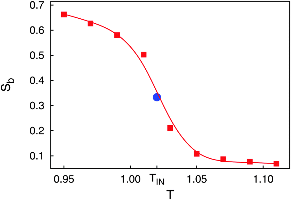 | ||
Fig. 1 Plot of the nematic order parameter Sb as a function of temperature T ( ). Data are shown for N = 1000 mesogens. The IN phase transition occurs at TIN and is obtained from an analysis of the second-order cumulant (see text). The full line represents a spline fitted to the discrete data points and intended to guide the eye. Also shown is SIN = ⅓ at TIN predicted by LdG theory ( ). Data are shown for N = 1000 mesogens. The IN phase transition occurs at TIN and is obtained from an analysis of the second-order cumulant (see text). The full line represents a spline fitted to the discrete data points and intended to guide the eye. Also shown is SIN = ⅓ at TIN predicted by LdG theory ( ) (see text). ) (see text). | ||
Another well-known finite-size effect is visible in the isotropic phase (i.e., for T > TIN) where Sb approaches a small nonzero plateau value of about 0.069. This can be explained by assuming that the liquid crystal consists of molecular-size domains in which mesogens align their longer axes preferentially because of the form of φmm. In the isotropic phase these domains are uncorrelated. However, their number is finite so that by averaging Sb over the ordered domains a residual nonzero value is obtained.
At this stage it is noteworthy that finite system size affects the nematic order parameter only in the isotropic phase and near the IN phase transition [see, for example, Fig. 6(b) of ref. 12 or Fig. 2(b) of ref. 31] whereas Sb is insensitive to system size sufficiently deep in the nematic phase. Hence, under the present thermodynamic conditions (see Section 4.1) a significant system-size effect is not anticipated for the pure host phase (i.e., in the absence of colloidal particles). The presence of the colloids will cause formation of nearly isotropic domains of a certain size determined by the surface curvature of the colloidal particle (i.e., by its size). In these domains, S(r) is small but nonzero. However, size and shape of the domains and the actual value of S(r) reflect the true physics of the system and should not be confused with finite-size effects in the bulk and in the absence of the colloids as discussed before.
Another feature illustrated by the plot in Fig. 1 is that the value predicted by LdG theory
 | (26) |
To estimate TIN (and therefore SIN) we resort to FSS theory and compute g2 from eqn (25) using  for three system sizes corresponding to N = 500, N = 1000, and N = 5000 mesogens. That data obtained for these system sizes are significant and meaningful is concluded from the much more detailed analysis of the IN phase transition in the present model conducted earlier by Greschek and Schoen.31
Results of the present calculations displayed in Fig. 2 indicate that above TIN (i.e., in the isotropic phase), g2 turns out to be independent of system size as one would expect according to the scaling behavior of 〈Sb〉 ∝ N−1/2 and that of 〈Sb2〉 ∝ N−1.26,31 As one approaches TIN from above, g2 first passes through a maximum if N is sufficiently large and then declines sharply with decreasing T where in the nematic phase g2 turns out to be the smaller the larger N is. Most importantly, however, all three curves plotted in Fig. 2 pass through a common intersection demarcating TIN ≃ 1.02 according to the discussion in Section 3.2.3.
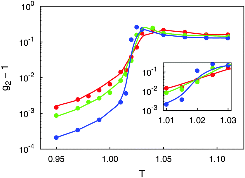 | ||
Fig. 2 Plots of second-order cumulants g2 as functions of temperature T for N = 500 ( ), N = 1000 ( ), N = 1000 ( ), and N = 5000 ( ), and N = 5000 ( ). Inset is an enlargement in the vicinity of the IN phase transition. ). Inset is an enlargement in the vicinity of the IN phase transition. | ||
Equipped with this result and with expressions for a, B, and C [see eqn (22a) and (22b)], we are now in a position to estimate T* where we find T*/TIN ≃ 0.746. For MBBA, Senbetu and Woo's experimental data allow us to estimate T*/TIN ≃ 0.904 which is of about the same order of magnitude.39 Thus, we conclude that our combined MMF DFT-LdG-FSS approach provides a sufficiently realistic description of the nematic host phase.
With the parameters T*, a, B, and C we plot the LdG free energy density Δf0 from eqn (13) in Fig. 3. As expected, the absolute minimum of Δf0 corresponds to the isotropic phase (Sb = 0) for T > TIN. Exactly at T = TIN, ΔfLdG exhibits a double minimum, one at Sb = 0, the other one at Sb > 0 in the nematic phase. The depth of both minima is the same, that is isotropic and nematic phases coexist. At T slightly below TIN the depth of the minimum at Sb > 0 exceeds that at Sb = 0 so that the nematic phase is thermodynamically stable whereas the isotropic phase is only metastable. Finally, at T = T* the plot of Δf0 exhibits a saddle point at Sb = 0 indicating that the isotropic phase is unstable for all T ≤ T*.
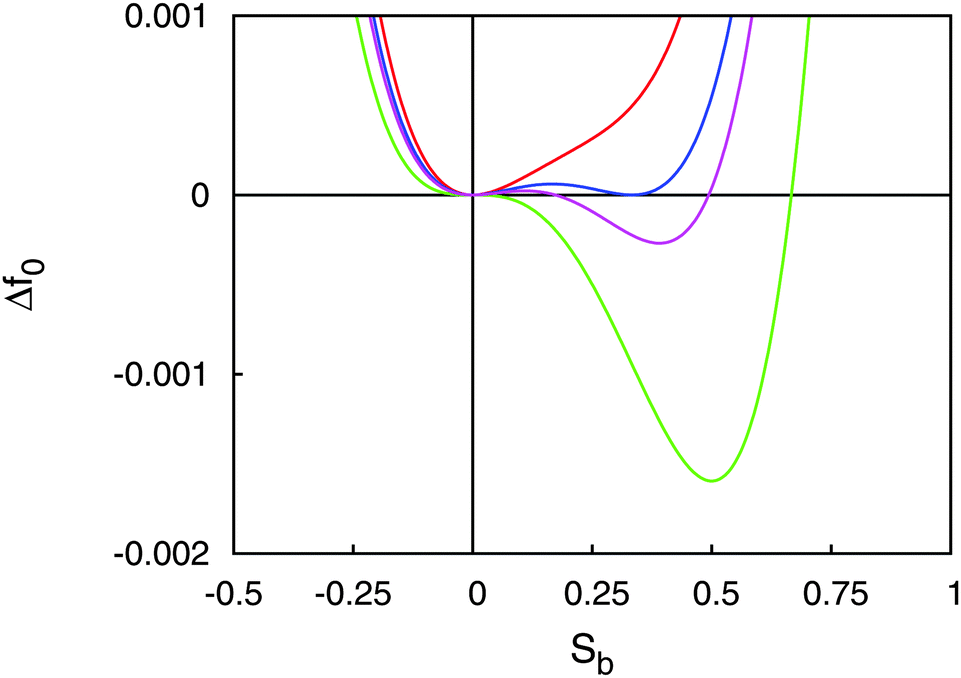 | ||
Fig. 3 Plot of the change in LdG free energy density ΔfLdG as a function of the nematic order parameter S for T > TIN ( ), T = TIN ( ), T = TIN ( ), T < TIN ( ), T < TIN ( ), and T = T* ( ), and T = T* ( ). ). | ||
4.3 Core region
Turning now to our composite system in which colloids are immersed into the nematic host phase, we begin by considering a single colloidal particle first. Plots of the local nematic order parameter S(r) and the director field(r) in Fig. 4(a) reveal the formation of a defect near the colloid's north pole and that this defect is of the Boojum topology as anticipated for a locally planar anchoring of mesogens at the colloid's surface. Upon entering this region, S(r) declines sharply so that the defect has a well-defined boundary.
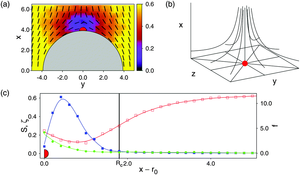 | ||
Fig. 4 (a) Director field (r) (dashes) and local nematic order parameter S(r) (see attached color bar) projected onto the x–y plane. The grey semicircle marks the upper hemisphere of a colloidal particle with part of a Boojum defect topology centered on its north pole. (b) Three-dimensional sketch of the variation of (r) for a hyperbolic hedgehog defect topology. (c) Variation of S(r) (left ordinate,  ), the Frank–Oseen contribution fFO(r) [right ordinate, ), the Frank–Oseen contribution fFO(r) [right ordinate,  , see eqn (14)], and the biaxial order parameter ζ(r) (left ordinate, see text, , see eqn (14)], and the biaxial order parameter ζ(r) (left ordinate, see text,  ) as functions of x − r0 and z = 0 cutting through the defect core. Notice that the data plotted have been averaged over a strip of width δy = 1.2 centered on y = 0 to get a reasonably smooth variation of all three quantities shown. The vertical solid line marks the radius Rcore of the circular defect core. Red marks have been added to all three parts of the figure to assist the reader in relating them. ) as functions of x − r0 and z = 0 cutting through the defect core. Notice that the data plotted have been averaged over a strip of width δy = 1.2 centered on y = 0 to get a reasonably smooth variation of all three quantities shown. The vertical solid line marks the radius Rcore of the circular defect core. Red marks have been added to all three parts of the figure to assist the reader in relating them. | ||
As already mentioned in Section 3.1, special precaution has to be taken to treat the contribution of the defect core to Δf(r). Within the defect core the variation of (r) bears a lot of structural similarity with a hyperbolic hedgehog defect in the bulk [see Fig. 4(b)] represented by (r) = (x, y, −z)T where superscript T denotes the transpose.
Moreover, plots in Fig. 4(c) show that outside the defect core both S(r) and fFO(r) vary rather weakly. Hence, the assumption underlying eqn (14), namely the variation of (r) on a length scale exceeding the molecular one, is well justified. Therefore, fel ≈ fFO outside the defect core to a good approximation [see eqn (14)].
Inside the defect core, however, (r) varies on a molecular scale such that fFO passes through a relatively sharp maximum and then declines sharply as one approaches the center of the core region [see Fig. 4(c)] so that the assumption underlying fFO(r) is no longer justified. To account for the free-energy contribution of the defect core we therefore resort to a procedure suggested earlier by Lubensky et al.20
These authors derive an analytic expression for the free energy of defect cores considering analytical director fields (such as the one for the hyperbolic hedgehog defect) [see eqn (8) of ref. 20]. Because of the plots in Fig. 4(a) and (b) we take half of this free energy and assign it to a spherical core volume ![[/]](https://www.rsc.org/images/entities/char_e12a.gif) πRcore3 to obtain a free-energy density of fcore = K/Rcore2 where Rcore is the radius of a circular Boojum defect core. We determine the size of the core region by cutting through the center of the defect core of an isolated colloid along the x-axis and take as Rcore that value of x at which S(r) drops below SIN for the first time. Using Rcore ≃ 1.80 [see Fig. 4(c)] we obtain fcore ≈ 0.50kBT which is not an unrealistic value as we conclude by comparison with the much more sophisticated DFT study of defect-core free-energy densities of de las Heras et al.22
πRcore3 to obtain a free-energy density of fcore = K/Rcore2 where Rcore is the radius of a circular Boojum defect core. We determine the size of the core region by cutting through the center of the defect core of an isolated colloid along the x-axis and take as Rcore that value of x at which S(r) drops below SIN for the first time. Using Rcore ≃ 1.80 [see Fig. 4(c)] we obtain fcore ≈ 0.50kBT which is not an unrealistic value as we conclude by comparison with the much more sophisticated DFT study of defect-core free-energy densities of de las Heras et al.22
To approximate the free-energy density of more complex defect topologies to be discussed in Section 4.4 we assume that fcore is the same everywhere in the core region irrespective of the defect topology. Hence, the free energy of the defect core is obtained from the expression
 | (27) |
through a three-dimensional integration of Δf(r) along the x-, y-, and z-axis using a simple trapezoidal rule.
However, it needs to be stressed that this is truly only a rough approximation to the free energy of defect cores even though it is a standard one in the literature.20,33 Perhaps the most significant assumption behind the expression in eqn (27) is that of insensitivity of fcore to variations in the topology of defects as illustrated by plots in Fig. 4. To improve this situation one could in principle invoke the approach of Lubensky et al.20 and try to find an analytic expression for (r) inside the defect core such that for each and every topology observed a different fcore might obtain analytically. However, if and to what an extent this is possible is currently unknown and would require a study in its own right.
Nevertheless, we feel that the assumption of a assigning the same constant fcore regardless of the specific defect topology is not unrealistically crude. This is concluded from the work of Lubensky et al.20 who show that even for rather disparate (r) the free energy of the defect core is more or less the same such that core ∝ Vcore to a reasonable degree.
4.4 The effective interaction potential
Based upon results presented in Sections 4.2 and 4.3 we now focus on the effective interaction between a pair of colloids immersed in the nematic bulk host phase. We begin in Fig. 5 by considering a pair of colloids in contact with each other. Plots (a)–(c) in the upper panel of Fig. 5 indicate that part of the Boojum defects at isolated colloids interact at sufficiently close proximity of these colloids. For example, for an angle θ = 0° between the intercolloidal center of mass distance r12 and the far-field nematic director0 a toroidal defect structure exists surrounding the point of contact between the colloids. As θ increases this torus is first “ripped apart” and eventually a handle-like structure forms at θ = 90°.
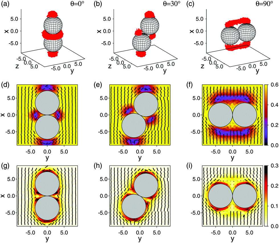 | ||
| Fig. 5 Upper panel (a)–(c) shows plots of the three-dimensional defect topologies of a pair of colloids (grey spheres) immersed in a nematic host fluid for various angles θ between the center-of-mass distance vector r12 and the far-field nematic director 0 given in the plots. Defect regions are colored in red subject to the condition S(r) ≤ ⅓. Plots in the middle panel (d)–(f) show the corresponding local director field (dashes) and the local nematic order parameter (see attached color bar) projected onto the x–y plane where grey circles are similar two-dimensional projections of the colloids. Plots of the biaxiality order parameter are shown in the lower panel (g)–(i). In all cases 0·êx = 1. | ||
Plots (d)–(f) in the middle panel of Fig. 5 are projections of (r) onto the x–y plane for the same angles as in parts (a)–(c) of the same figure. These plots indicate that (r) = 0 except in the immediate vicinity of the colloidal pair. As one approaches the colloids, (r) is deformed with respect to 0.
Finally, we plot in parts (g)–(i) of Fig. 5 the local biaxiality order parameter ζ(r). We compute this quantity from our MC simulations via the smallest and middle eigenvalue of Q(r) in eqn (17) which can be expressed as λ− = −[S(r) + ζ(r)]/2 and λ0 = −[S(r) − ζ(r)]/2, respectively, for a system with biaxial symmetry because TrQ(r) = 0. From Fig. 5(g)–(i) one notices that biaxiality is relatively small and restricted to the immediate vicinity of the colloids' surfaces. We ascribe this to the nanoscopic size of our colloids (i.e., to the large curvature of their surfaces). A comparison with plots in Fig. 5(d)–(g) illustrates the structural similarity between both sets of plots. More specifically, where S(r) is lowest, ζ(r) is largest.
This also offers another route to treating core at least in principle because the plots in Fig. 5 suggest that inside the defect core Q(r) remains non-singular. Instead of invoking the approximations introduced in Section 4.3 one could therefore try to use directly Q(r) from eqn (17) obtained in the MC simulations and plug it into the right-hand side of the expression on the first line of eqn (14). The required differentiation of Q(r) has, of course, to be performed numerically but would allow one to compute fel(r) also inside the defect core.
Unfortunately, in practice we found that our data are way too noisy to follow this route and obtain reliable values for fel(r) inside the defect core. A reliable numerical differentiation of Q(r) would need a much finer discretization of the grid on which this quantity is stored because of its rather strong spatial variation inside the defect core. Notice, that this does not contradict the smoothness of plots in Fig. 4(c) as the data shown there have been averaged over a fairly wide strip inside the defect core.
The magnitude of the spatial variation of Q(r) is reflected in part by the plot of fFO(r) in Fig. 4(c) sufficiently deep inside the defect core. In this region, fFO(r) exceeds its typical values in the elastic regime just outside this region by about two to three orders of magnitude. As is clear from eqn (14) the large value of fFO(r) can immediately be traced back to a very strong spatial variation of (r) inside the defect core which is linked to a similarly strong spatial variation of Q(r) because of eqn (9).
Consequently, to be able to differentiate this quantity numerically and reliably would require a better resolution of Q(r) on a much finer grid. This obviously would entail much longer MC simulations to obtain reasonably good statistics which, unfortunately, is beyond reach given the number of simulations and the typical system sizes necessary to map out the effective interaction potential between the colloidal pair with sufficient resolution. Because of these constraints and because of the discussion in Section 4.3 we conclude that our present treatment of the free-energy contribution of the defect core offers the best possible approximation.
In addition to a distortion of (r) plots in Fig. 5(d)–(f) reveal regions in which S(r) ≪ Sb. From the parallel three-dimensional plots in Fig. 5(a)–(c) one sees that the volume of these regions changes with θ. Hence, it seems intuitive to introduce an associated change in effective free energy
| Δeff = el + core + ΔLdG − 2ΔB | (28) |
B is the change in free energy associated with a single Boojum defect. In computing ΔB we assume that it also consists of an elastic Frank, a defect-core, and a LdG free energy contribution. In practice, it turns out that the contribution of each of the first three terms on the right-hand side of eqn (28) for the interacting colloidal pair relative to the corresponding contribution to ΔB is roughly of the same order of magnitude in the range of kBT in agreement with plots presented in Fig. 6 and in Fig. 7.
 | ||
Fig. 6 The effective free energy Δeff in units of the change in free energy associated with an isolated Boojum colloid ΔB. Vertical dashed lines demarcate minima in the curves plotted; the limiting value θ ≈ 49° is also indicated (see text); r12 = 7.20 ( ), r12 = 8.00 ( ), r12 = 8.00 ( ). ). | ||
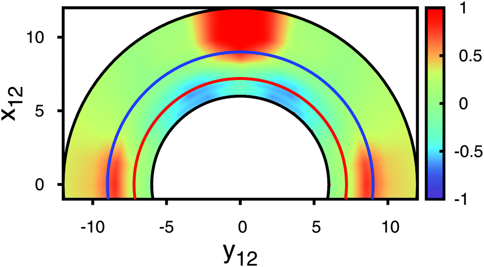 | ||
Fig. 7 Contour plot of Δeff/ΔB (see attached color bar) as a function of rT12 = (x12, y12, 0)T. Curves plotted in Fig. 6 correspond to r12 = 7.20 ( ) and to r12 = 8.00 ( ) and to r12 = 8.00 ( ), respectively. ), respectively. | ||
Data for Δeff plotted in Fig. 6 exhibit a number of interesting features. First, one notices that depending on θ, the sum el + core + ΔLdG may be larger or smaller than 2ΔB and therefore Δeff may be viewed as a repulsive or attractive effective interaction potential acting between a colloidal pair and mediated by the nematic host phase. Second, the minimum in the plot of Δeff shifts to larger angles θmin as the intercolloidal center-of-mass distance increases. This is fully in line with experimental observations made by Smalyukh et al.11 and theoretical observations made by Tasinkevych et al.8 Third, these latter authors could also demonstrate that their experimental value of θmin increases monotonically towards a limiting value. This limiting value is found by realizing that for a single Boojum defect (corresponding to a sufficiently separated pair of colloids) the spatial variation of the nematic director field bears close resemblance to the spatial variation of the electrostatic field associated with interacting quadrupoles. For the latter the orientation dependence of the electrostatic energy can be cast as
| U ∝ 9 − 90cos2θ+ 105cos4θ | (29) |
One also notices from the plots in Fig. 6 an upward shift of the curves that causes larger spatial regions in which the effective potential Δeff is repulsive. In particular, such a repulsive region exists for angles θ ≳ 70° and r12 = 8.00. This is fully in line with trajectories of colloids measured by Smalyukh et al.11 by video microscopy and presented in their Fig. 2.
From curves such as the ones presented in Fig. 6 we are now in a position to present in Fig. 7 a more refined contour plot of Δeff illustrating in a broader way the structural complexity of the effective-potential landscape.
Using the data plotted in Fig. 7 we can now also investigate structures that several colloids would form in a nematic host phase. For simplicity, and because the experiments used a quasi two-dimensional setup11 we consider a two-dimensional, coarse-grained system treating the nematic host implicitly via Δeff. To account for the evolution of the colloids in configuration space we employ a conventional canonical-ensemble Metropolis MC scheme.
To that end we store Δeff on a two-dimensional regular grid with a spacing of 0.2 between neighboring nodes. As a position of a colloid will normally not coincide with a grid point, we interpolate Δeff between the four nearest-neighbor grid points in a bilinear fashion to get Δeff at the actual center-of-mass position of a colloidal disk. A displacement of a disk is then accepted with a probability min[1, exp(−Δeff/ΔB)].
For two packing fractions ϕ = Ncollπr02/sxsy of Ncoll colloidal disks, characteristic “snapshots” from the simulations at thermodynamic equilibrium are shown in Fig. 8. Here sx and sy are linear dimensions of the simulation cell. As one can see colloidal disks tend to form linear chains at the lower packing fraction where the symmetry axis of each chain forms an angle of θ ≈ 30° with 0 [see Fig. 8(a)] whereas at higher packing fraction a more extended two-dimensional network of colloidal disks exists at thermodynamic equilibrium [see Fig. 8(b)]. Both types of structures bear a remarkable resemblance to those displayed in Fig. 1(b) and (e) of the work by Smalyukh et al.11
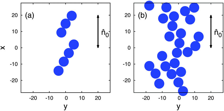 | ||
| Fig. 8 “Snapshots” from canonical-ensemble MC simulations of colloidal disks immersed in a nematic host phase taken into account implicitly via the effective interaction potential Δeff shown in Fig. 7. (a) ϕ = 0.065, (b) ϕ = 0.234 (sx = sy = 50 and 0·êx = 1). The direction of the far-field director 0 is indicated in the figure. | ||
5 Discussion and conclusions
By means of a novel hybrid approach we investigate the self-assembly of spherical colloidal particles with chemically homogeneous surfaces at a coarse-grained level of description. Our hybrid approach combines molecular-scale methods and theories such as MC computer simulations, classical DFT, and elements of FSS theory with macroscopic theories such as LdG and the Frank–Oseen treatment of the free-energy density associated with elastic deformations of the director field. The goal of this approach is to integrate out less relevant degrees of freedom in a controlled fashion while maintaining the correct physics of a composite system such as the present one. The philosophy of our approach is quite general and may perhaps be applied to other composite systems as well. An example in this respect could be that of Janus colloids immersed into a nematic host phase.In our case, the colloids are immersed into a nematic liquid-crystal host phase. Self-assembly is driven by effective interactions mediated by the host. The effective interactions correspond to a change in free energy caused by defects (i.e., regions of lower nematic order) in the host phase. These defects cause a local decline of nematic order and distortion of the director field. Both features arise because of the mismatch between the local alignment of mesogens at the curved surface of the colloids and the nematic far-field director 0. They depend on the arrangement of the colloids in space.
We are treating both the local lowering of nematic order and the distortion of the director field at mean-field level assuming that the former can be adequately accounted for by LdG theory and the latter within the standard expression for the Frank elastic free energy. The mean-field character is reflected by the fact that we compute LdG expansion parameters a, B, and C from mean-field DFT and that the elastic contribution to the change in free energy does not account for fluctuations of (r). However, the Frank free energy is computed only outside the defect core where (r) changes on a length scale large compared to a molecular one.
Applying LdG theory within the framework of molecular simulations poses a fundamental problem because under most conditions statistical accuracy is insufficient to compute the LdG expansion coefficients B and C.26 However, employing classical DFT allows one to express analytically the LDG coefficients in terms of thermodynamic state parameters such as density and temperature.
A key ingredient in LdG theory is the temperature T* at which the isotropic phase becomes thermodynamically unstable. It is related to the temperature TIN at which one has IN phase coexistence. To improve our DFT estimate of T* for the LdG treatment we locate TIN through an analysis of second-order cumulants of the nematic order parameter within the framework of FSS theory.
An alternative route to the LdG coefficients has recently been proposed by Gupta and Ilg.40 Starting from a state point in the isotropic phase for which they can compute the free energy semi-analytically, Gupta and Ilg apply an external ordering field to drive the system into an ordered nematic phase. In the ordered state the free energy can then be calculated by thermodynamic integration. The intrinsic free-energy contribution can be related to functions that can, on the one hand, be determined numerically through reliable fit functions and that one can, on the other hand relate to the LdG expansion coefficients analytically.
A crucial ingredient in the approach of Gupta and Ilg is the ordering field which for their Gay–Berne model of a liquid crystal has a magnitude of the order of one. When applying the technique of Gupta and Ilg to our model system we found that the magnitude of the ordering field had to be about five orders of magnitude larger to drive a system from the isotropic to the nematic phase. We believe that this huge difference in the external field is caused by the almost spherical shape of mesogens in our model. Because of the disparate magnitude of the ordering fields it turned out that for the present model the approach of Gupta and Ilg could not be applied reliably.
However, our combined MC-DFT-FSS approach allows us to compute the effective interaction potential reliably. A comparison with experimental data reveals that
(1) the effective potential has a minimum at an angle θ ≈ 30° between the intercolloidal distance vector r12 and the far-field nematic director 0 if the colloids are sufficiently close to each other.
(2) the position of the minimum shifts monotonically to larger θ if r12 increases.
(3) depending on θ and r12 the effective potential may be repulsive or attractive.
These features turn out to be in semi-quantitative agreement with experimental observations.9,11
Encouraged by the apparent consistency of these observations with experimental data we perform coarse-grained, canonical-ensemble MC simulations of several colloidal disks immersed in a nematic host phase that is now treated implicitly through the effective interaction potential. In that regard our approach has a multiscale character. The structures observed at different packing fractions agree again qualitatively with experimental data11 despite the much larger colloids used experimentally.
However, it needs to be stressed that the simulations of several colloids is based upon the assumption of pairwise additivity of the effective interactions. A priori there is no guarantee that this assumption is valid. However, the excellent qualitative agreement between structures observed within our approach with those seen experimentalls seems to justfy the assumption of pairwise additive effective interactions a posteriori.
In summary, we have shown that the self-assembly of colloidal particles in a nematic liquid crystal is driven by the occurrence of colloid-induced defects associated with a local elastic distortion of the director field. This also implies that in an isotropic phase no such self-assembly would occur as the effective interaction potential would vanish identically.
Acknowledgements
We are grateful for financial support from the Deutsche Forschungsgemeinschaft via the International Graduate Research Training Group 1524.References
-
P. G. de Gennes and J. Prost, The physics of liquid crystals, Clarendon, Oxford, 2nd edn, 1995 Search PubMed
.
- V. S. R. Jampani, M. Škarabot, M. Ravnik, S. Čopar, S. Žumer and I. Muševič, Phys. Rev. E: Stat., Nonlinear, Soft Matter Phys., 2011, 84, 031703 CrossRef CAS PubMed
- K. Izaki and Y. Kimura, Phys. Rev. E: Stat., Nonlinear, Soft Matter Phys., 2013, 87, 062507 CrossRef PubMed
- U. Ognysta, A. Nych, V. Nazarenko, M. Škarabot and I. Muševič, Langmuir, 2009, 25, 12092–12100 CrossRef CAS PubMed
- H. Qi and T. Hegmann, J. Mater. Chem., 2006, 16, 4197–4205 RSC
- M. Humar, M. Ravnik, S. Pajk and I. Muševič, Nat. Photonics, 2009, 3, 595–600 CrossRef CAS
- I. Muševič, M. Škarabot and M. Humar, J. Phys.: Condens. Matter, 2011, 23, 284112 CrossRef PubMed
- M. Tasinkevych, N. M. Silvestre and M. M. Telo da Gama, New J. Phys., 2012, 14, 073030 CrossRef
- P. Poulin and D. Weitz, Phys. Rev. E: Stat. Phys., Plasmas, Fluids, Relat. Interdiscip. Top., 1998, 57, 626–637 CrossRef CAS
- P. Poulin, H. Stark, T. C. Lubensky and D. A. Weitz, Science, 1997, 275, 1770–1773 CrossRef CAS PubMed
- I. I. Smalyukh, O. D. Lavrentovich, A. N. Kuzmin, A. V. Kachynski and P. N. Prasad, Phys. Rev. Lett., 2005, 95, 157801 CrossRef CAS PubMed
- S. Giura and M. Schoen, Phys. Rev. E: Stat., Nonlinear, Soft Matter Phys., 2014, 90, 022507 CrossRef PubMed
- W. Maier and A. Saupe, Z. Naturforsch., A: Phys. Sci., 1958, 13, 564–566 Search PubMed
- W. Maier and A. Saupe, Z. Naturforsch., A: Phys. Sci., 1959, 14, 882–889 Search PubMed
- B. Jérôme, Rep. Prog. Phys., 1991, 54, 391–451 CrossRef
- M. Škarabot, M. Ravnik, S. Žumer, U. Tkalec, I. Poberaj, D. Babič, N. Osterman and I. Muševič, Phys. Rev. E: Stat., Nonlinear, Soft Matter Phys., 2008, 77, 031705 CrossRef PubMed
-
A. A. Sonin, The Surface Physics of Liquid Crystals, Gordon and Breach, Amsterdam, 1995 Search PubMed
- M. Melle, S. Schlotthauer, M. G. Mazza, S. H. L. Klapp and M. Schoen, J. Chem. Phys., 2012, 136, 194703 CrossRef PubMed
- R. W. Ruhwandl and E. M. Terentjev, Phys. Rev. E: Stat. Phys., Plasmas, Fluids, Relat. Interdiscip. Top., 1997, 56, 5561–5566 CrossRef CAS
- T. C. Lubensky, D. Pettey, N. Currier and H. Stark, Phys. Rev. E: Stat. Phys., Plasmas, Fluids, Relat. Interdiscip. Top., 1998, 57, 610–625 CrossRef CAS
- S. Grollau, N. L. Abbott and J. J. de Pablo, Phys. Rev. E: Stat., Nonlinear, Soft Matter Phys., 2003, 67, 011702 CrossRef CAS PubMed
- D. de las Heras, L. Mederos and E. Velasco, Liq. Cryst., 2010, 37, 45–56 CrossRef CAS
- I. Bajc, F. Hecht and S. Žumer, 2015, arXiv:1505.07046v1.
- J. Dontabhaktuni, M. Ravnik and S. Žumer, Soft Matter, 2012, 8, 1657–1663 RSC
- I. Muševič, U. Škarabot, U. Tkalec, M. Ravnik and S. Žumer, Science, 2006, 313, 954–958 CrossRef PubMed
- R. Eppenga and D. Frenkel, Mol. Phys., 1984, 52, 1303–1334 CrossRef CAS
-
W. H. Press, S. A. Teukolsky, W. T. Vetterling and B. P. Flannery, Numerical recipes, Cambridge University Press, Cambridge, 3rd edn, 2007 Search PubMed
- M. P. Allen and D. Frenkel, Phys. Rev. A: At., Mol., Opt. Phys., 1988, 37, 1813R–1816R CrossRef
- M. P. Allen and D. Frenkel, Phys. Rev. A: At., Mol., Opt. Phys., 1990, 42, 3641 CrossRef
- T. Stieger, M. Schoen and M. G. Mazza, J. Chem. Phys., 2014, 140, 054905 CrossRef PubMed
- M. Greschek and M. Schoen, Phys. Rev. E: Stat., Nonlinear, Soft Matter Phys., 2011, 83, 011704 CrossRef PubMed
- S. Giura, B. G. Márkus, S. H. L. Klapp and M. Schoen, Phys. Rev. E: Stat., Nonlinear, Soft Matter Phys., 2013, 87, 012313 CrossRef PubMed
-
M. Kleman and O. D. Lavrentovich, Soft Matter Physics: An introduction, Springer-Verlag, New York, 2003 Search PubMed
- H. Weber, W. Paul and K. Binder, Phys. Rev. E: Stat. Phys., Plasmas, Fluids, Relat. Interdiscip. Top., 1999, 59, 2168–2174 CrossRef CAS
- K. Vollmayer, J. D. Reger, M. Scheucher and K. Binder, Z. Phys. B: Condens. Matter, 1993, 91, 113–125 CrossRef
-
D. Frenkel and B. Smit, Understanding molecular simulation: From algorithms to applications, Academic Press, San Diego, 2nd edn, 2002 Search PubMed
-
M. P. Allen and D. J. Tildesley, Computer simulation of liquids, Oxford University Press, Oxford, 2002 Search PubMed
- W. Maier and A. Saupe, Z. Naturforsch., A: Phys. Sci., 1960, 15, 287–292 Search PubMed
- L. Senbetu and C.-W. Woo, Mol. Cryst. Liq. Cryst., 1982, 84, 101–124 CrossRef CAS
- B. Gupta and P. Ilg, Polymers, 2013, 5, 328–343 CrossRef
| This journal is © The Royal Society of Chemistry 2016 |