High-accuracy QSAR models of narcosis toxicities of phenols based on various data partition, descriptor selection and modelling methods

Abstract

The environmental protection agency thinks that quantitative structure–activity relationship (QSAR) analysis can better replace toxicity tests. In this paper, we developed QSAR methods to evaluate the narcosis toxicities of 50 phenol analogues. We first built multiple linear regression (MLR), stepwise multiple linear regression (SLR) and support vector regression (SVR) models using five descriptors and three different partitions, and the optimal SVR models with all three training-test partitions had the highest external prediction ability, about 10% higher than the models in the literature. Second, to identify more effective descriptors, we applied two in-house methods to select descriptors with clear meanings from 1264 descriptors calculated by the PCLIENT software and used them to construct the MLR, SLR and SVR models. Our results showed that our best SVR model (R_pred² = 0.972) significantly increased 16.55% on the test set, and the appropriate partition presented the better stability. The different partitions of the training-test datasets also supported the excellent predictive power of the best SVR model. We further evaluated the regression significance of our SVR model and the importance of each single descriptor of the model according to the interpretability analysis. Our work provided a valuable exploration of different combinations among data partition, descriptor selection and model and a useful theoretical understanding of the toxicity of phenol analogues, especially for such a small dataset.

---

1. Introduction

Along with rapid economic development, environmental issues, especially chemical-related environmental issues, are becoming increasingly prominent.¹ As their natural biodegradation and complete mineralization rates are very slow,² phenolic compounds are looked upon as the priority among environmental pollutants. Phenol is a toxic, carcinogenic and mutagenic aromatic pollutant^3,4 that is produced and discharged by many industries such as petroleum refining, petrochemical, pharmaceutical and resin-manufacturing plants. Therefore, phenol is the major pollutant found in the wastewaters of these industries.^5–7 Chemical and physical processes can be used for the recovery of phenol from the wastewaters, but the first thing to know is the toxic effects of these phenolic compounds. So an appropriate assessment approach to determine the risk from chemicals is very relevant.

Traditionally, the quantitative structure–activity relationship (QSAR) has been perceived as a means of establishing a correlation between chemical structure and biological activity, and it contributes to explaining how structural descriptors determine biological activity.^5,8–10 In particular, an acceptable QSAR model is considered as a rapid and cost-effective alternative to experimental evaluation. The mathematical methods for constructing QSAR include linear and nonlinear methods that solve regression and classification problems in data structure.¹¹ Baker et al.¹² have reported a QSAR study of the toxicity of alkylated or halogenated phenols. In that study, they developed a simple model for phenol toxicity based on physicochemical properties without external prediction. Based on the same dataset, Xu et al.¹³ calculated descriptors directly from the phenol molecular structures and used two approaches, multiple linear regression (MLR) analysis and feed-forward neural networks, to develop a model. Guo and Xu¹⁴ also used the same approaches to demonstrate that neural networks were better than MLR in prediction. However, regardless of neural networks or MLR, traditional modelling methods based on the principle of empirical minimization have many flaws. The support vector machine (SVM) based on statistical theory and minimum structure risk is not only helpful to preferably solve certain problems, such as the small-sample, nonlinear, dimension disaster and local minimum problems, but is also helpful to provide a strong generalization ability.¹⁵ SVM includes support vector classification and support vector regression (SVR), and SVR is more applicable to develop QSAR models.¹⁶

There is a widespread concern over big datasets, but small datasets are inevitable in many fields. On the basis of our previous work,¹⁷ we further evaluate the effectiveness and application of methods in coping with small datasets. We found out the literature dataset is a typical one, and several different groups continuously researched it using their different methods. So, we developed the SVR models using the same toxicity dataset in the present work. To select more appropriate descriptors, we employed two methods developed in-house based on SVR: the worst descriptor elimination multi-roundly (WDEM)¹⁸ and the high-dimensional descriptors selection nonlinearly (HDSN).¹⁹ We further utilized SVR to build more effective models based on the obtained descriptors, and used MLR and stepwise multiple linear regression (SLR) to build the reference model. Our analysis will offer some theoretical references to predict the activities of several phenol compounds.

2. Material and methods

2.1 Data set

We took the data set with 50 known phenol toxicities used in the paper from the work of Baker et al.¹² and Guo and Xu¹⁴ (Table 1). The toxicities were expressed as log BR, the negative logarithm of the IGC₅₀ (50% growth inhibitory concentration) values in millimoles per liter.

Table 1 Phenols and their related toxicities

No.	Compound	log BR(expt.)	No.	Compound	log BR(expt.)
1	Phenol	−0.431	26	2,5-Dichlorophenol	1.128
2	2,6-Difluorophenol	0.396	27	2,3-Dichlorophenol	1.271
3	2-Fluorophenol	0.248	28	4-Chloro-2-methyl phenol	0.700
4	4-Fluorophenol	0.017	29	4-Chloro-3-methylphenol	0.795
5	3-Fluorophenol	0.473	30	2,4-Dichlorophenol	1.036
6	4-Methylphenol	−0.192	31	3-tert-Butylphenol	0.730
7	3-Methylphenol	−0.062	32	4-tert-Butylphenol	0.913
8	2-Chlorophenol	0.277	33	3,5-Dichlorophenol	1.562
9	2-Bromophenol	0.504	34	2-Phenylphenol	1.094
10	4-Chlorophenol	0.545	35	2,4-Dibromophenola	1.403
11	3-Ethylphenol	0.229	36	2,3,6-Trimethylphenol	0.418
12	2-Ethylphenol	0.176	37	3,4,5-TrimethylphenoI	0.930
13	4-Bromophenol	0.681	38	2,4,6-Trichlorophenol	1.695
14	2,3-Dimethylphenol	0.122	39	4-Chloro-3,5-dimethylphenol	1.203
15	2,4-Dimethylphenol	0.128	40	4-Bromo-2,6-dichlorophenol	1.779
16	2,5-Dimethylphenol	0.009	41	2,4,5-TrichlorophenoI	2.100
17	3,4-Dimethylphenol	0.122	42	4-Bromo-6-chloro-2-methylphenol	1.277
18	3,5-Dimethylphenol	0.113	43	4-Bromo-2,6-dimethylphenol	1.278
19	3-Chloro-4-fluorophenol	0.842	44	2,4,6-Tribrmophenol	2.050
20	2-Chloro-5-methylphenol	0.640	45	2-tert-Butyl-4-methylphenol	1.297
21	4-Iodophenol	0.854	46	4-Chloro-2-isopropyl-5-methylphenol	1.862
22	3-Iodophenol	1.118	47	6-tert-Butyl-2,4-dimethylphenol	1.245
23	2-Isopropylphenol	0.803	48	2,6-Diphenylphenol	2.113
24	3-Isopropylphenol	0.609	49	2,4-Dibromo-6-phenylphenol	2.207
25	4-Isopropylphenol	0.473	50	2,6-Di-tert-butyl-4-methylphen	1.788

---

2.2 Molecular descriptors and descriptors selection

To develop a powerful predictor for a QSAR model, one of the keys is to formulate the effective descriptors that can truly reflect their intrinsic correlation with the attribute. So, we used two sets of descriptors to test the performance of the descriptor selection methods and used two sets of descriptor selection methods to enhance the performance of QSAR models.

2.2.1 The low-dimensional descriptor space. The low-dimensional descriptor space includes 2 volume parameters (V and V²), 2 hydrophobic parameters (log P and log² P) and 1 topological parameter (A_m3). The literature adopted these 5 descriptors calculated by a multivariate statistical analysis program package to construct QSAR models.¹⁴

2.2.2 The high-dimensional descriptor space and descriptors selection. The high-dimensional descriptor space encodes much more structural information. Twenty-four groups of different descriptor calculation modules of the software PCLIENT (http://www.vcclab.org/lab/pclient/) can generate about 3000 descriptors²⁰ (Table 2). We can add the molecular structures of compounds stored into SMILES format to the PCLIENT for calculating descriptors in the default state.

Table 2 Groups and counts of descriptors from the software PCLIENT²¹

Group	Group of descriptors	Count	Group	Group of descriptors	Count
1	Constitutional descriptors	48	13	RDF descriptors	150
2	Topological descriptors	119	14	3D-MoRSE descriptors	160
3	Walk and path counts	47	15	WHIM descriptors	99
4	Connectivity indices	33	16	GETAWAY descriptors	197
5	Information indices	47	17	Functional group counts	121
6	2D autocorrelations	96	18	Atom-centered fragments	120
7	Edge adjacency indices	107	19	Charge descriptors	14
8	BCUT descriptors	64	20	Molecular properties	28
9	Topological charge indices	21	21	ET-state indices	>300
10	Eigenvalue-based indices	44	22	ET-state properties*	3
11	Randic molecular profiles	41	23	GSFRAG descriptor	307
12	Geometrical descriptors	74	24	GSFRAG-L descriptor	886
Total: >3000

---

2.2.3 Descriptors selection methods. Although these descriptors possess a majority of the information on the compounds, the sharp increase in descriptor dimensions is adverse for accurate modelling. And there is a consensus that not all descriptors contribute to building a good model. To select the most useful descriptors rapidly and efficiently, our laboratory devised two sets of techniques for reducing the dimensionality, which were successfully applied to the data of antitumor activity^21,22 and phenol toxicity.¹⁷

Firstly, we screened all the descriptors coarsely and nonlinearly by HDSN.¹⁹ In this method, the original training set was arranged as (y, x), including n samples and m descriptors. A K*m controlled matrix with the number of K such as 500 was generated in this paper. The matrix consists of an equal number of randomly positioned 1s and 0s per column, representing whether the descriptor in that column was included in the modelling or not. Then a tenfold cross-validation with SVR on the training set was conducted for each row of the matrix using only the descriptors corresponding to 1 s in the row. The importance of a descriptor was judged based on contrasting the prediction accuracy of two sets of models, one set with the descriptor included and the other with the descriptor excluded. The accuracy was defined as the mean square error (MSE) of the constructed model. Because the controlled matrix was random, the optimal descriptors subset might be a different result in each implementation. We conducted the descriptor selection 20 times on the training set and obtained 20 sets of optimal descriptors.

Then we further screened each set of descriptors carefully using the worst descriptor elimination multi-roundly method (WDEM).¹⁸ The matrix was arranged as (y_i, x_ij), i = 1,2, …, n, j = 1,2,…, m′, including n samples and m′ descriptors. In the first round, the original MSE₀ was computed by leave-one-out (LOO) cross-validation with SVR, and then the corresponding MSE_j were obtained by successively wiping out the j^th descriptor. When min (MSE_j) ≤ MSE₀, the corresponding descriptor would be removed and entered into the next round of screening instead of ending the filter.

2.3 Model development

We developed models using the linear regression methods (MLR and SLR) implemented in the statistical software DPS data processing system²³ and the nonlinear regression method (SVR),¹⁵ respectively.

2.4 Model evaluation

There are some examples from the published QSAR models, which, in spite of their high fitted accuracy for the training sets, fail to be sufficiently rigorous for the validation tests. Independent testing is a rigorous modelling approach in which the test set is not used in the descriptor selection and model construction steps. The phenol toxicities in the test set are unknown for the actual prediction, and another important reason is that it would generate an overly optimistic estimation for the external prediction if the test set was involved in descriptor selection. Therefore, we used the independent test set to evaluate the performance of the proposed model because rigorous validation was a crucial, integral component of the QSAR model development. Furthermore, to investigate whether the different partitioning influenced the performance of a predictor, we conducted three dataset partitions (Table 3).

Table 3 Different partition in training-test sets

	Compounds in the training set	Compounds in the test set
1^st partition	1–45	46–50
2^nd partition^14	Remaining samples	4, 23, 26, 34 and 44
3^rd partition^13	Remaining samples	16, 33, 35, 44 and 45

---

We assessed the predictive capacity of the models based on MSE and the squared predictive correlation coefficient (R_pred²) values calculated by the following equations:

y_i = experimental values in the test set, ŷ_i = predicted values in the test set, n = the number of the test set, ȳ_train = the mean activity values of the training set.

Generally, researchers considered that an outstanding QSAR model should have a lower strong MSE²⁴ and higher R_pred² (>0.5).²⁵

3. Results and discussion

3.1 Comparative QSAR modelling with the low-dimensional descriptors using SLR, MLR and SVR methods

Guo and Xu¹⁴ constructed QSAR models by MLR methods and considered the five descriptors V, V², log P, log² P and A_m3 as the critical factors for predicting phenol narcosis toxicities. To compare the learning ability and generalization ability of the SVR, SLR and MLR methods, we validated the QSAR models using the fitting test and the independent test on these literature descriptors. And to avoid the overfitting problem of the small dataset with 50 samples, we conducted three different partitions with the same ratio of 45 to 5, and got three groups of training-test sets. In addition, we trained SVR models by LOO cross-validation and modelled in five kernel functions (t = 0; t = 1, d = 2; t = 1, d = 3; t = 2 and t = 3). The results based on the low-dimensional literature descriptors showed that: (1) the optimal SVR models with all three training-test partitions had a higher predictive ability than MLR (lg BR = 0.852 − 1.764V + 1.031V² + 2.269 lg P − 1.165 lg² P + 0.207A_m3) in the fitting test and the independent test; (2) SLR with the same descriptors had a similar fitting predictive ability occasionally, but a lower independent predictive ability than SVR; (3) the performance of the SVR predictor with t = 0 was the best for the 1^st partition, the performance of the SVR predictor with t = 2 was the best for the 2^nd partition and the performance of the SVR predictor with t = 1, d = 3 was the best for the 3^rd partition in the independent test; and (4) the best QSAR models from the three partitions presented the similar performance, and their generalization abilities in the independent test were about 10% better than the one from MLR provided in the literature¹⁴ (Table 4).

Table 4 Comparative QSAR models of the literature dataset based on three methods and three training-test partitions^a

			SVR					MLR	SLR
			t = 0	t = 1, d = 2	t = 1, d = 3	t = 2	t = 3
a Notes: the bold indicated the best results in each case.
1^st partition	External	MSE	0.099	80.517	442.585	0.323	40.172	0.772	0.326
		Rpred^2	0.925	−59.663	−332.450	0.757	−29.266	0.551	0.920
	Internal	MSE	0.022	0.031	0.029	0.022	0.044	0.317	0.146
		Rpred^2	0.937	0.910	0.916	0.937	0.874	0.711	0.938
2^nd partition	External	MSE	0.040	0.051	0.099	0.039	0.056	0.276	0.207
		Rpred^2	0.913	0.890	0.786	0.915	0.879	0.834	0.907
	Internal	MSE	0.027	0.131	0.039	0.025	0.045	0.241	0.157
		Rpred^2	0.939	0.697	0.910	0.943	0.895	0.865	0.943
3^rd partition	External	MSE	0.065	0.067	0.052	0.064	0.070	0.377	0.238
		Rpred^2	0.904	0.900	0.922	0.905	0.895	0.788	0.915
	Internal	MSE	0.025	0.137	0.027	0.025	0.026	0.302	0.154
		Rpred^2	0.939	0.667	0.935	0.939	0.936	0.777	0.942

---

These results indicated that SVR with a suitable kernel function was a powerful technique for a given set of low-dimensional descriptor space, and that kernel function selection would be effective for more accurate predictions.

3.2 Comparative QSAR modelling with the high-dimensional descriptors using SLR, MLR and SVR methods

3.2.1 Descriptors selection and retention. We calculated a total of 1264 descriptors by PCLIENT for each compound, and then used the high-dimensional dataset containing the independent variables (all 1264 descriptor values) and the dependent variables [log BR_(expt.) values] for modelling. Since the high-dimensional descriptors possessed redundant information, we developed two novel methods (HDSN and WDEM) based on SVR to select the more critical ones nonlinearly from the thousands of descriptors. In each partition, we repeated the descriptor selection 20 times due to the stochastic screening process of the HDSN method. Using the HDSN method 20 times, we obtained 60 training sets and descriptors of the training sets reduced to 19–40 after four to ten rounds of selection. Using the WDEM method, we further removed redundant descriptors after no more than 13 selection rounds. Thus, we obtained 60 groups of reserved descriptors with the minimum MSE values. Finally, we developed and evaluated 300 SVR models with five kernel functions and LOO cross-validation, 60 MLR models and 60 SLR models for the test set based on the reserved descriptors. We numbered the all SVR models according to theR_pred² value as follows because of the value's importance in the external prediction for modelling (Table 5).

Table 5 Top five best SVR models in three kinds of partitions^a

		Indices	SVR1	SVR2	SVR3	SVR4	SVR5
a SR, screening rounds; ON, obtained number; BKF, best kernel function.
1^st partition	HDSN	SR	9	7	9	9	6
		ON	27	20	21	21	30
	WDEM	SR	11	4	7	6	10
		ON	16	16	14	15	20
	Models	BKF	t = 3	t = 2	t = 0	t = 2	t = 2
		Rpred^2	0.959	0.955	0.949	0.941	0.939
2^nd partition	HDSN	SR	7	10	4	8	8
		ON	25	19	40	26	23
	WDEM	SR	8	8	10	8	10
		ON	17	11	30	18	13
	Models	BKF	t = 2	t = 0	t = 2	t = 3	t = 2
		Rpred^2	0.977	0.972	0.968	0.965	0.960
3^rd partition	HDSN	SR	5	10	9	9	5
		ON	39	22	23	23	40
	WDEM	SR	13	5	7	7	5
		ON	26	17	16	16	35
	Models	BKF	t = 1, d = 2	t = 2	t = 1, d = 2	t = 1, d = 2	t = 2
		Rpred^2	0.996	0.987	0.973	0.967	0.967

---

Not every model makes good sense, so we only analyzed the effective models whose R_pred² values were greater than or equal to 0.5. In particular, we only chose the model with the best kernel function but not every kernel function for every repetition. Therefore, we got 20 models for every partition. The retention probability of the effective SVR models referred to the ratio of the effective models to the 20 times repetition. The statistical result showed that (1) in the case of three training-test partitions, the probabilities of effective models from SLR increased by 5% to 15% over the ones from MLR, and the ones from SVR increased by 5% to 35%; (2) the probabilities of effective models in the two literature partitions (the 2^nd partition and the 3^rd one) were higher. The appearance suggested that the SVR method can construct more effective models than the others and the literature can provide important guidance on selecting the training-test partition (Table 6).

Table 6 Retention probability of effective models

	1^st partition	2^nd partition	3^rd partition
SVR	95%	100%	100%
SLR	75%	90%	100%
MLR	60%	80%	95%

---

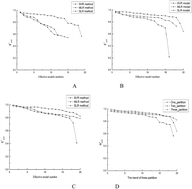
To compare the external predictive ability of SLR, MLR and SVR in more detail, we discussed the changed trend of the retention models. We conducted trend analysis through the R_pred² values of the retention models, since the models with higher R_pred² values had stronger generalization ability. In order to observe the general trend of the retention models with different partitions and different methods, we sorted the retention models according to their R_pred² values and then drew Fig. 1. From this it appeared that: (1) with three partitions, SVR had more advantages than the other two methods in predictive ability, and the advantages were not only in the amount of the retention model but also in the assessed value; (2) after putting the best SVR models for every set of descriptors together observing the three partitions, the top 15 models all performed similarly well, and the third partition presented the best stability.

Fig. 1 Analysis of the modeling advantages of the first (A), the second (B), the third (C) and the best (D) classification.

Because of the varying quantity of retention models with the different training-test partitions and different modelling methods, direct comparison of retention model trends could not demonstrate the pros and cons of the methods objectively and comprehensively. Therefore, we further analyzed the significant test of R_pred² difference for all the retention models in each partition statistically comparing the modelling methods. The result indicated that the difference between SVR and MLR reached a significant level in the third partition, and the difference between SVR and SLR reached a highly significant level in the first and the third partitions (Table 7 and Fig. 2).

Table 7 P value of the statistical test^a

	1^st partition		2^nd partition		3^rd partition
	SVR	MLR	SVR	MLR	SVR	MLR
a Notes: ** represented highly significant; * represented significant.
MLR	0.126		0.058		0.017*
SLR	0.004**	0.191	0.180	0.179	0.010**	0.315

---

Fig. 2 The difference of R_pred² from each model in three kinds of classification.

3.2.2 Retained descriptors after screening. There is reached consensus that not all descriptors are necessary to build a good model, so we adopted our in-house descriptor selection methods based on SVR, called HDSN and WDEM to screen the key descriptors. The two methods supporting the selected descriptors were closely associated with the dependent variables [log BR_(expt.) values]. However, these were numerous since different retention models possessed different sets of descriptors. Here we chose to retained descriptors more than 10 times under a single partition, or above 8 times the descriptors under two or more partitions in all the retention models. For comparative analysis of the descriptor reserved situation, we calculated the relative retention probability of descriptors using the number of selected descriptors divided by the number of retained models in the various partitions. The result demonstrated that Mor16e, DISPe, Mor16u, MATS3e and G(O..Cl) simultaneously appeared in three partitions and the frequencies of occurrence were the highest (Fig. 3). Based on the above result, we concluded that these five descriptors were crucially important for the narcosis toxicity of phenolic compounds.

Fig. 3 Relative probability of high frequency descriptors from three partitions.

3.2.3 Establishing an interpretability system for the best model. We chose the SVR2 model in the 2^nd partition (SVR2_2) and the SVR1 model in the 3^rd partition (SVR1_3) for the optimal candidates from Table 5, because the SVR1_3 model had the best R_pred² (= 0.996) and the SVR2_2 model had the fewest descriptors (=11). But the SVR1_3 model had 26 descriptors, and too many more descriptors could lead to high computational complexity and incline to an overfitting phenomenon. More important was that the model with many more descriptors would fail in practical applicability. In conclusion, we considered the SVR2_2 model as the best one in our work.

Many previous research results have indicated that SVR has better generalization but poorer interpretability in some nonlinear fields. So, aiming at this weak point, our research group established a complete set of an interpretability system for SVR based on F-tests in the previous studies.²⁶ According to the interpretability analysis of the SVR2_2 model, we obtained the significance of the regression model and the importance of single indicators based on SVR and the F-test. The results showed that the nonlinear regression of the SVR2_2 model (R_pred² = 0.972) was highly significant because its F-value (4461.81) was greater than F_0.05(11, 33).

We listed the obtained descriptors of phenols compounds from the SVR2_2 model in Table 8, and the algorithms supported the indication that all these descriptors played the most important roles in describing the narcosis activity of these compounds. For all the descriptors in the SVR2_2 model, the analysis of single-factor effects showed that the narcosis activity was highly significantly negative correlated with BLTD48 values, but highly significantly positively correlated with 10 other descriptor values (Table 8 and Fig. 4).

Table 8 Definition and importance analysis of the descriptors in the SVR2_2 model^a

Group name	Descriptor name	F-Value
a *, 0.01 < p < 0.05; **, p < 0.01; F0.05(1, 10) = 4.96; F0.01(1, 10) = 10.04; F0.05(1, 25) = 4.24; F0.01(1, 25) = 7.77; F0.05(26, 18) = 2.13; F0.01(26, 18) = 2.97; F0.05(11,33) = 2.09; F0.01(11, 33) = 2.84.
Molecular properties	BLTD48: Verhaar model of Daphnia base-line toxicity from MLOGP (mmol l^−1)	19 289.250**
Geometrical descriptors	G(O..Cl): sum of geometrical distances between O..Cl	4461.810**
GETAWAY descriptors	H7e: H autocorrelation of lag 7/weighted by atomic Sanderson electronegativities	2839.560**
GETAWAY descriptors	HTm: H total index/weighted by atomic masses	2477.360**
GETAWAY descriptors	R5v+: R maximal autocorrelation of lag 5/weighted by atomic van der Waals volumes	2430.070**
Topological descriptors	PHI: Kier flexibility index	1345.930**
Information indices	CIC3: complementary information content (neighborhood symmetry of 3-order)	1327.350**
3D-MoRSE descriptors	Mor16ez: 3D-MoRSE − signal 16/weighted by atomic Sanderson electronegativities	1140.060**
RDF descriptors	RDF040p: radial distribution function − 4.0/weighted by atomic polarizabilities	1082.480**
Walk and path counts	SRW01: self-returning walk count of order 01 (number of non-H atoms, nSK)	1017.870**
2D autocorrelations	MATS3e: Moran autocorrelation − lag 3/weighted by atomic Sanderson electronegativities	626.600**

---

Fig. 4 Single-factor effect of descriptors in the SVR2_2 model.

In previous studies, BLTD48,²⁷ G(O..Cl),²⁸ H7e,²⁹ HTm,^30,31 PHI,^32–34 CIC3,^35–37 Mor16ez,^38,39 RDF040p,²¹ SRW01 (ref. 40) and MATS3e^21,41 have been reported as modeling descriptors, but the fifth important descriptor R5v+ and this combination of descriptors have never been mentioned. In our SVR2_2 model, the most important descriptor BLTD48 is one of the molecular properties, and the toxicity has decreased with increasing its structure in phenolic compounds;²⁷ the second important descriptor G(O..Cl) is one of the geometrical descriptors, and has been used to predict the tertiary structure of α-glucosidase and inhibition properties of N-(phenoxydecyl) phthalimide derivatives;²⁸ the third important descriptor H7e is one of the GETAWAY descriptors and has been selected by the genetic algorithm to model the HIV-1 RT inhibitory activity and MT4 blood toxicity;²⁹ the fourth important descriptor HTm is also one of the GETAWAY descriptors and has been selected to model the design of potent antimalarial bisbenzamidines³⁰ and to predict activity coefficients at infinite dilution of hydrocarbons in aqueous solutions.³¹ Particularly, HTm provides information on the degree of interaction between all the molecule atoms, determined by the atomic masses of every individual atom in the molecule;³⁰ the sixth important descriptor PHI is one of the topological descriptors and has been found to improve the prediction ability.^33,34 The PHI is a measure of molecular flexibility. When the molecular flexibility of a molecule increases, the resistance of molecule against changes increases and its molecular diffusivity decreases;³² the seventh important descriptor CIC3 is one of the information indices, and has been developed for predicting anti-HCV activity of thiourea derivatives³⁶ and nonlinear relationships between retention time and molecular structure of peptides originating from proteomes.³⁷ CIC3 depicts the topological features of atoms based on neighborhood environment;³⁵ the eighth important descriptor Mor16ez is a 3D-molecule representation of structures based on electron diffraction (3D-MoRSE) descriptor weighted by electronegativity, and has been used to develop QSAR models.^38,39 It illustrates the role of geometry of the peptide molecules and their electrical diffraction properties during the interaction with the binding site of the receptor;³⁸ the ninth important descriptor RDF040p is one of the RDF descriptors and has been selected to model as an important feature;²¹ the tenth important descriptor SRW01 is one of the walk and path counts, and has been selected as a feature that weighted most heavily at the ends of PC1 of physico-chemical space;⁴⁰ the last important descriptor MATS3e is classified in the Moran autocorrelation descriptors, and it is calculated using the average value of a special property of a molecule and the number of vertex pairs at a topological distance. Therefore, the MATS3e has the length three in the lag (the prescribed length or topological distance that connects a pair of atoms) and bear the atomic Sanderson electronegativities as the weighting scheme.^21,41

These results might help to explain how the descriptors could determine the narcosis activity of phenols, and to improve and exploit the physical and chemical technology for environmental chemical pollutants. Based on the above results, it is confirmed that we can construct some ideal QSAR models that should be capable of accurately predicting several groups of the desired property for a newly synthesized or a hypothetical molecule. In addition, the descriptors selection methods and the modelling techniques from our studies cannot only be applied to develop and improve the control of phenols, but also be applied to all the fields of small molecules modelling.

4. Conclusion

Without the need for geometry structure optimization, the structural information of 50 known phenol toxicities could be described using 1264 molecular descriptors which were easily offered by the PCLIENT. Using two nonlinear descriptor selection methods and three training-test partitions, we obtained 60 groups of important descriptors and used them in our QSAR analysis. We demonstrated that the nonlinear SVR models using selected descriptors performed better than the linear reference models on test dataset in terms of prediction accuracy. Our results offer new theoretical tools and new descriptors for chemical design and the development of phenols, especially for such small datasets.

Conflict of interest

There is no conflict of interest.

Acknowledgements

This research was supported by the National Natural Science Foundation for Young Scientists of China (No. 31301388), China Postdoctoral Science Foundation (No. 2015T80870 and No. 2014M562109). The authors also thank Ran Li and Ying He at Department of Bioinformatics, Hunan Agricultural University, Changsha, China for their help during the manuscript preparation.

References

1. H. Wang, Z. Yan, H. Li, N. Yang, K. M. Y. Leung, Y. Wang, R. Yu, L. Zhang, W. Wang, C. Jiao and Z. Liu, Environ. Pollut., 2012, 165, 174–181.
2. M. C. Tomei, M. C. Annesini and A. J. Daugulis, New Biotechnol., 2012, 30, 44–50.
3. H. Ucun, E. Yıldız and A. Nuhoğlu, Bioresour. Technol., 2010, 101, 2965–2971.
4. M. Bajaj, C. Gallert and J. Winter, Bioresour. Technol., 2008, 99, 8376–8391.
5. X. L. Li, Z. Y. Wang, H. L. Liu and H. X. Yu, Bull. Environ. Contam. Toxicol., 2012, 89, 27–31.
6. D. Abd-El-Haleem, H. Moawad, E. A. Zaki and S. Zaki, Microb. Ecol., 2002, 43, 217–224.
7. K. Watanabe, S. Hino and N. Takahashi, J. Ferment. Bioeng., 1996, 82, 522–524.
8. V. Aruoja, M. Sihtmäe, H. C. Dubourguier and A. Kahru, Chemosphere, 2011, 84, 1310–1320.
9. M. K. Sharma, P. R. Murumkar, G. Kuang, Y. Tang and M. R. Yadav, RSC Adv., 2016, 6, 1466–1483.
10. Y. Pan, T. Li, J. Cheng, D. Telesca, J. I. Zink and J. Jiang, RSC Adv., 2016, 6, 25766–25775.
11. S. Pirhadi, F. Shiri and J. B. Ghasemi, RSC Adv., 2015, 5, 104635–104665.
12. L. L. Baker, S. K. Wesley and T. W. Schultz, Proceedings Third International Workshop on Quantitative Structure–Activity Relationships in Environmental Toxicology, 1988, pp. 165–168.
13. L. Xu, J. W. Ball, S. L. Dixon and P. C. Jurs, Environ. Toxicol. Chem., 1994, 13, 841–851.
14. M. Guo and L. Xu, Acta Sci. Circumstantiae, 1998, 18, 122–127.
15. V. N. Vapnik, The Nature of Statistical Learning Theory, Springer-Verlag, 1995, pp. 87–189.
16. L. Ji, X. D. Wang, X. S. Yang, S. Liu and L. Wang, Chin. Sci. Bull., 2008, 53, 33–39.
17. W. Zhou, S. B. Wu, Z. J. Dai, Y. Chen, Y. Xiang, J. R. Chen, C. Y. Sun, Q. M. Zhou and Z. M. Yuan, Chemom. Intell. Lab. Syst., 2015, 145, 30–38.
18. X. S. Tan, Z. M. Yuan, T. J. Zhou, C. J. Wang and J. Y. Xiong, Chem. J. Chin. Univ., 2008, 29, 95–99.
19. Z. J. Dai, W. Zhou and Z. M. Yuan, Acta Phys.–Chim. Sin., 2011, 27, 1654–1660.
20. I. V. Tetko, J. Gasteiger, R. Todeschini, A. Mauri, D. Livingstone, P. Ertl, V. A. Palyulin, E. V. Radchenko, N. S. Zefirov, A. S. Makarenko, V. Y. Tanchuk and V. V. Prokopenko, J. Comput.-Aided Mol. Des., 2005, 19, 453–463.
21. W. Zhou, Z. J. Dai, Y. Chen, H. Y. Wang and Z. M. Yuan, Int. J. Mol. Sci., 2012, 13, 1161–1172.
22. W. Zhou, Z. J. Dai, Y. Chen and Z. M. Yuan, Med. Chem. Res., 2013, 22, 278–286.
23. Q. Y. Tang and M. G. Feng, DPS Data Processing System – Experimental Design, Statistical Analysis and Data Mining, Science Press, 2007, pp. 625–644.
24. Y. Chen, Z. M. Yuan, W. Zhou and X. Y. Xiong, Acta Phys.–Chim. Sin., 2009, 25, 1587–1592.
25. S. X. Zhang, L. Y. Wei, K. Bastow, W. F. Zheng, A. Brossi, K. H. Lee and A. Tropsha, J. Comput.-Aided Mol. Des., 2007, 21, 97–112.
26. L. F. Wang, X. S. Tan, L. Y. Bai and Z. M. Yuan, Asian J. Chem., 2012, 24, 1575–1578.
27. K. Dieguez-Santana, H. Pham-The, P. J. Villegas-Aguilar, H. Le-Thi-Thu, J. A. Castillo-Garit and G. M. Casañola-Martin, Chemosphere, 2016, 165, 434–441.
28. M. Pooyafar and D. Ajloo, Acta Chim. Slov., 2012, 59, 221–232.
29. M. Cruz-Monteagudo, H. PhamThe, M. N. D. S. Cordeiro and F. Borges, Mol. Inf., 2010, 29, 303–321.
30. M. Cruz-Monteagudo, F. Borges, M. P. González and M. N. D. S. Cordeiro, Bioorg. Med. Chem., 2007, 15, 5322–5339.
31. G. Astray, J. Morales, M. González-Temes, J. C. Mejuto and A. J. Magdalena, Mediterr. J. Chem., 2015, 3, 1073–1082.
32. M. Sattari and F. Gharagheizi, Chemosphere, 2008, 72, 1298–1302.
33. T. P. J. Villalobos, R. G. Ibarra and J. J. M. Acosta, J. Mol. Graphics Modell., 2013, 46, 105–124.
34. M. Goodarzi, L. dos Santos Coelho, B. Honarparvar, E. V. Ortiz and P. R. Duchowicz, Ecotoxicol. Environ. Saf., 2016, 128, 52–60.
35. R. Pal, M. A. Islam, T. Hossain and A. Saha, Sci. Pharm., 2011, 79, 461–477.
36. N. Khatri, V. Lather and A. K. Madan, Chemom. Intell. Lab. Syst., 2015, 140, 13–21.
37. P. Žuvela, K. Macur, J. J. Liu and T. Bączek, J. Pharm. Biomed. Anal., 2016, 127, 94–100.
38. A. Kyani, M. Mehrabian and H. Jenssen, Chem. Biol. Drug Des., 2012, 79, 166–176.
39. A. Pogorzelska, J. Sławiński, K. Brożewicz, S. Ulenberg and T. Bączek, Molecules, 2015, 20, 21960–21970.
40. R. M. Khan, C. H. Luk, A. Flinker, A. Aggarwal, H. Lapid, R. Haddad and N. Sobel, J. Neurosci., 2007, 27, 10015–10023.
41. H. Tavakoli and J. B. Ghasemi, J. Comput. Sci., 2015, 11, 112–120.

---

Footnote

† These authors contributed equally to this work.

---