A GMDH-type neural network with multi-filter feature selection for the prediction of transition temperatures of bent-core liquid crystals

Abstract

A novel strategy for the prediction of the transition temperature of bent-core liquid crystals (LCs) based on the combination of multi filter feature selection and group method of data handling (GMDH) type neural networks is reported. An entire set of 243 compounds was randomly divided into a training set of 207 compounds and a test set of 36 compounds. Descriptors were selected from a pool of 2D, and two pools of 2D and 3D ones, optimized by molecular mechanics (MM) and semi-empirical (SE) method. The reduction of the pool of descriptors was performed using multi filters based on chi square and v-WSH algorithm, while the final subset selection was performed by GMDH algorithm during the learning process. The obtained 2D, MM and SE GMDH models have 11, 13 and 16 descriptors, respectively, and demonstrate good generalization and predictive ability (R² = 0.92). The final models were subjected to a randomization test for validation purpose. Those models appear to be not only suitable for prediction, but they also allow the identification of key structural features that alter the transition temperature of bent-core LCs.

---

Introduction

Liquid crystal (LC) molecules share important properties of both liquids and crystals: they flow like a liquid and at the same time maintain some degree of positional and/or orientational order.¹ As such, they have unique physicochemical properties and consequently wide application in various fields.^2,3 But, in order to be used in any particular technological application, thermotropic LCs have to possess stable mesophases in a suitable temperature range.⁴ The upper temperature limit (i.e. transition temperature) at which mesophase exists can be used as a measure of its stability.⁵

Quantitative structure–property relationship (QSPR) methodology has been often used to predict various physical and chemical properties of LCs.^4–10 Artificial neural networks (ANNs), as a nonlinear modelling approach, are mostly used for this purpose, due to complex relationships exist between a property of molecule and its structure.⁶ Among first, Johnson and Jurs⁴ have shown that the clearing temperatures of a series of structurally similar rod-like LCs can be successfully predicted using ANNs. In a recent study, Antanasijević et al. have used QSPR method in combination with ANNs, decision trees (DTs) and MARS (multivariate adaptive regression splines) technique for the prediction of liquid crystallinity,¹⁰ and with DT and MARS for the estimation of the clearing temperatures⁷ of five-ring bent-core molecules.

Feature selection is an important step in QSPR development, concerning that a large number of molecular descriptors (up to two thousands) can be calculated for each structure.¹¹ In general, a large pool of descriptors can be reduced using filter, wrapper or embedded feature selection methods. Filter techniques eliminate irrelevant and redundant features by checking data consistency,¹² while wrappers evaluate the usefulness of an input set during the model training.¹³ Embedded methods perform variable selection in the process of training and they are specific to given learning machines.¹⁴ Since filters work much faster, they are suitable for large datasets, while wrapper and embedded methods achieve excellent accuracy at the cost of significant time.¹⁵ In recent years, hybrid approaches are proposed in order to combine the advantages of both methods.^16,17

It is generally more convenient to have a linear or polynomial QSPR model that enables analysis of particular descriptor contribution and therefore group method of data handling (GMDH) type neural networks can be used as an alternative to standard ANNs, which operates like a ‘black box’ model.¹⁸

GMDH is a specific type of feed-forward ANNs, which algorithm was firstly introduced by Ivakhnenko¹⁹ and enhanced by others.²⁰ The GMDH-type ANNs, often referred to as polynomial neural networks, are based on the identification of the functional structure of a model, which is extracted from the empirical data by polynomial functions.²¹ Therefore, a nonphysical model, with high accuracy and simpler structure than a corresponding physical model, can be obtained by applying GMDH on complex (non-linear) input–output relationships, especially if the available dataset is small and noisy inputs are present.²²

In the last decade, GMDH has been used to solve complex engineering problems and to identify the behaviour of nonlinear systems in many fields, such as control engineering, data mining, process optimization, and medical image recognition and diagnosis (see studies^23–26 and reference cited therein).

In this study, we report the development of QSPR model using GMDH-type neural network for the prediction of the transition temperatures of five-ring bent-core LCs. Although GMDH operates as an embedded feature selection method, chi square ranking and correlation filter were applied in the pre-processing step in order to reduce the pool of descriptors and to enhance the descriptor selection process. To date, this is the first application of GMDH-type neural networks for the prediction of LC properties.

Computational methods

Dataset

A recently published dataset (see Table S1 in the supplemental material of paper by Antanasijević et al.⁷), which contains transition temperature values for 243 bent-core LC compounds, was utilized for the development and testing of GMDH models. In this dataset the transition temperatures were in the range from 352.15 to 458.15 K. The dataset consisted of structurally diverse five-ring aromatic compounds in the terms of the type of linkage groups and their orientation, substituents on the rings, and the type and length of terminal chains. The same subset of 36 compounds was used for model testing, in order to allow direct comparison with the models created in the previous study.⁷

Structure optimization and descriptor generation

The molecular structures were firstly sketched in ChemDraw software, and then initially optimized using MMFF94 optimization routine (ChemAxon, Marvin²⁷). The final geometry of the minimum energy conformation was obtained using the semi-empirical PM3 method (Polak–Ribiere algorithm) using HyperChem8.0 program.²⁸ The structures were optimized at the restricted Hartree–Fock level until the RMS gradient was 0.01 kcal Å⁻¹ mol⁻¹.

In order to check the accuracy of the applied optimisation methods, the obtained structures were compared with available optimized structures from DFT studies. For example, the DFT study²⁹ for the compound 161 indicates that bending angle (α), which determines molecular packing and therefore its transition temperature, has the value of 121°. The α of 125° and 126° obtained in this study for the same compound by MM and SE method, respectively, is in the fair agreement with the abovementioned DFT value.

Subsequently, the calculation of molecular descriptors was performed using PaDEL-Descriptor software.³⁰ After the elimination of descriptors with constant and near constant values, the pool of 501 constitutional, topological, geometric, electrostatic and hybrid descriptors (360 2D and 141 3D) was remained.

Descriptor selection

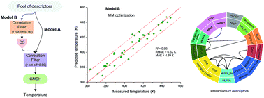
The feature selection was performed as presented in Fig. 1a:

Fig. 1 (a) Strategies for the selection of descriptors (b) the number of descriptors selected in each step. CF90 and CF99 stand for correlation filter with r cut-off equal to 0.90 and 0.99, respectively.

(a) The A models were created using correlation filter (CF) in order to eliminate collinear descriptors (r > 0.90), after which GMHD is used to select the best subset of descriptors during learning (embedded feature selection);

(b) The B models were created using multi filter approach that combines a chi square (CS) ranking in the first step with a collinear based elimination of descriptors in the second step, after which, in the third step, GMHD was used as embedded method. Prior the use of CS, near constant and highly correlated (r > 0.99) descriptors were removed in order to reduce redundant and non-useful information.³¹

The V-WSP variable reduction algorithm, proposed by Ballabio et al.,³² was used as correlation filter. This filter is an adaptation of the WSP (Wootton, Sergent, Phan-Tan-Luu's) algorithm, which was developed for space-filling designs of experiments and has been modified with the aim to select a representative set of variables instead of points.³² A Java implementation of this algorithm (the V-WSP tool) by Ambure et al.³³ has been used in this study.

The CS is a supervised univariate feature selection method that ranks the molecular descriptors according to their statistical association with the modelled output, where larger CS values imply more significant descriptors. A CS feature selection implementation in Statistica³⁴ was used, and because the CS is an association measure for categorical variables, the software's default number of bins (ten) was used for the chi square discretizing of molecular descriptors.³⁵

The final step in the both feature selection approaches is the application of GMDH, which has been proved to be effective with neural network classifiers.¹²

GMDH-type neural network

The GMDH algorithm, details of which can be found in literature,³⁶ differs from standard regression analysis and it is “similar to the way in which nature evolves by natural selection”.³⁷ There is a variety of supervised GMDH algorithms:³⁸ combinatorial algorithm, multilayered iterative algorithm (MIA), harmonical algorithm, objective system analysis, etc. Also, several enhancements related to the determination of structure, parameters and uncertainty of the GMDH models have been proposed in the recent years,^39,40 in order to increase their effectiveness for certain tasks. For example, unscented Kalman filter approach was applied for the design of GMDH model and determination of its uncertainty in order to obtain robust sensor and actuator for fault detection and diagnosis.^41,42

In this study, the MIA variant of GMDH that is implemented in NeuroShell 2 (ref. 43) was used. This is a self-organizing algorithm that uses the best polynomial terms (so-called “survivors”) from the first layer (eqn (1) and (2)) obtained by regressing pair of inputs (e.g. x₁ and x₂), as arguments in the next layer (eqn (3)).

The first layer

y₁ = a₁₀ + a₁₁x₁ + a₁₂x₂ + a₁₃x₁x₂ (1)

y₂ = a₂₀ + a₂₁x₃ + a₂₂x₄ + a₂₃x₃x₄ (2)

The next layer

z₁ = b₀ + b₁y₁ + b₂y₂ + b₃y₁y₂ (3)

As can be observed, the original inputs can be propagated thought the network without a construction of their polynomial form, which can reduce overall model complexity.

The layers were built until a certain stopping criterion was met. Over-fitting can be prevented using cross-validation or a statistical metric that penalize model complexity. In this study, the prediction squared error (PSE), introduced by Barron,⁴⁴ was applied as a stopping criterion, see eqn (4), where T_o is the observed temperature, T_p is predicted temperature, σ_o is output variance, k is the number of model parameters and N_p is the number of training data points.

In comparison with standard neural networks, the GMDH architecture (Fig. 2) is being fully adjusted both structurally and parametrically during training.⁴⁵ It is composed of an input layer, several hidden layers and an output layer. The number of input neurons is equal to the number of inputs, while each hidden layer consists of one or more neurons. Each hidden neuron is actually the resultant network that processes two inputs and generate one polynomial term.

Fig. 2 A typical architecture of GMDH-type neural network.

The input layer scales the descriptor values, while the first hidden layer performs the selection of descriptors. In the second, third and etc. hidden layers, higher order polynomials are being built. Since the number of survivors in the first hidden layer affects the diversity of final polynomial model and the quality of choice of important variables, the optimal maximum number of survivors (N^max_L1S) that are propagated to the second hidden layer needs to be defined.

N^max_L1S depends on the complexity of the problem, as well on the number of inputs presented to the GMDH. In order to empirically determine the optimal value of N^max_L1S in respect to the number of inputs, initial simulations with 2D descriptors were performed. The software that was used limits the value of N^max_L1S to 100, while in the case where the number of inputs (N_i) is lower than 50, the N^max_L1S is limited to twice N_i. The results obtained on cross-testing (with two datasets where each contained 20% of the original dataset) and N^max_L1S dependence of N_i are presented in Fig. 3. As can be observed, the dependence of N^max_L1S on N_i decreases with the increase of N_i, and can be approximated with linear/constant relationships in four regions.

Fig. 3 (a) Cross testing results (R_CT²) with datasets containing different numbers of inputs (b) the maximum number of polynomials (N^max_L1S) in the first layer of GMDH network depending on the number of inputs (N_i).

Other GMDH parameters that need to be defined prior to the training are the maximum number of descriptors in polynomials term, which was set to 4 for linear and to 3 for all other terms, and degree of polynomials, which was set to 3.

Results and discussion

The comparison of models

Both feature selection approaches were performed separately for each pool of descriptors (Fig. 1b). The number of CS ranked descriptors (150 and 200) that were to be further used was set to be about 50% higher that the number of descriptors that have remained after the application of correlation filter in the case of A models. The lowest ranked descriptor selected by GMDH in the case of 2D model had the rank of 136, while in the case of MM and SE the rank was 195 and 168, respectively. All three B models used lower number of descriptors in comparison with the corresponding A models.

The obtained A and B models were evaluated using Taylor diagram (Fig. 4). Taylor diagrams⁴⁶ provide a concise statistical summary of how well different models perform in the terms of their correlation (r), centered root mean square error (RMSE), and amplitude of their variations (standard deviations). Those three metrics are plotted simultaneously in the two-dimensional space using the following equation:

E² = σ_o² + σ_p² − 2σ_o²σ_p²r (5)

where E is the centered RMSE (eqn (6)), σ_o and σ_p are standard deviations of observed and predicted values, respectively.

Fig. 4 Taylor diagram for the A and B GMDH models.

In Fig. 4, it can be easily observed that the B models have lower error (i.e. centered RMSE) and higher correlation in comparison with the A models. Therefore, the applied multi filtered feature selection provides more accurate GMDH models than those obtained using the single correlation filter.

Regarding the B models, it can be seen that the models 2D and MM have almost the same centered RMSE and correlation, while the SE model has the standard deviation very similar to the observed one. In the next section, a detailed evaluation of the performance of B models is presented.

The GMDH parameters and performance metrics for B models are summarized in Table 1. The pool of 2D descriptors has been reduced to 19% of its initial size (from 360 to 70) after the multi filter feature selection was applied. A similar reduction of approximately 80% was obtained for the 2 & 3D models as well. All three models have the same number of hidden layers, but use a different number of descriptors which seems to correspond with the size of initial pool. The adjusted R² (0.92) and RMSE (6.68 ± 0.14 K) demonstrate that the generalization of all three QSPR models is statistically stable and that the models fit the test data well. The MM model performed slightly better, with the RMSE of 6.52 K, which is an improvement of 0.9 K in comparison with the results obtained in previous study⁷ using the MARS technique.

Table 1 GMDH parameters and the performance of B models

Pool of descriptors	Type		2D	MM (2 & 3D)	SE (2 & 3D)
a Number of hidden layers.b To access descriptors see Table 2.
	Ni		70	104	101
GMDH parameters	N^maxL1S		62	66	66
	NL^a		8	8	8
	Descriptors used^b (pool reduction)		11 (84%)	13 (88%)	16 (84%)
Performance metrics	Adjusted R^2		0.920	0.922	0.916
	F		401.7	414.7	372.9
	RMSE (K)		6.66	6.52	6.87
	Absolute error (K)	Min.	0.021	0.028	0.006
		Mean	5.15	4.89	5.02
		Max.	19.4	15.6	18.5

---

The Y-randomization was performed as an additional validation step in order to obtain an estimate of chance correlation.^47–52 The measured transition temperatures were shuffled by 10 random exchanges in their positions for each model, while the descriptors matrix has remained unchanged. In order to include the “selection bias”, as suggested by Rücker et al.,⁵³ randomized GMDH models were created using the same pool of descriptors and network parameters as the real ones. The risk of chance correlation was quantified by the value of R_p² that is calculated from the eqn (7) in which R_r² describes the training performance of randomized models, while R² stands for real QSPR models.⁵⁴ For a QSPR model having R_p² > 0.5, it may be considered that the model has not been obtained by chance alone.⁵⁵

For all models, the R_p² value was higher than 0.5 (Fig. 5), which indicates that they have passed the randomization test.

Fig. 5 Y-Randomization results.

Also, the real GMDH models have R² higher than the corresponding randomized models by more than 3 standard deviations (SD) (16 SD for 2D, 8 SD for MM and 11 SD for SE), which confirms their statistical significance at the 0.1% level.⁵³

As expected, the randomization results have shown that the risk of randomly obtained correlation increases with the size of pool of descriptors. Therefore, GMDH should be applied to the lowest possible pool of descriptors, and results suggest that the critical value is 115 descriptors (Fig. 5). On the other hand, it should be noted that the randomly correlated GMDH models can be easily identified, since all of them have more than 30 hidden layers and very complex polynomial equations.

The correlation between the experimental and predicted transition temperatures is shown graphically in Fig. 6a, where the outliers are also labelled. As can be seen from Fig. 6a, the compound 40 is an outlier in all three models, while the compound 42, which is from the same series, is an outlier only in the case of 2D model, but its transition temperature was also predicted with a higher error by both 2 & 3D models. Compounds 40 and 42 are from the series 38–42, which is structurally very similar to the series 29–37, the only difference being the orientation of the azomethine group (Fig. 6b). This small structural variation significantly alters the transition temperatures, i.e. corresponding homologues differ up to 30 K. This effect has not been captured by the selected descriptors, thus the predicted transition temperatures of those compounds correspond to their homologues from the series 29–37, which was more prevalent in the training set.

Fig. 6 (a) Measured vs. predicted plots with outliers. Solid lines represent the line of slope 1, while dashed lines indicate 3 SD error, (b) structure of outliers from the series 38–42, (c) structure and transition temperature of compounds from the series 50–58.

Regarding the compound 50, it exhibits an unexpectedly high transition temperature in comparison with its homologues from the same series (Fig. 6c), while in the case of compound 87 no obvious reason can be found for it to be an outlier.

The interpretation of descriptors

The eqn (8)–(10) were obtained using GMDH method with the pool of descriptors reduced by multi filter feature selection approach. In those equations, the descriptors are labelled according to the group they belong (Table 2), while in addition the 3D ones are marked with bold letters.

Table 2 List of descriptors with labels and short description

Group	Label (Eq. symbol)	Description
a Burden – CAS – University of Texas eigenvalue.b Molecular linear free energy relation.c Charged partial surface area.d Weighted holistic invariant molecular.
ALOGP	AlogP (Xa)	Ghose-Crippen LogKow
Barysz matrix	SM1_Dzi (Xb1)	Spectral moment of order 1 weighted by first ionization potential
	SM1_DzZ (Xb2)	Spectral moment of order 1 weighted by atomic number
	VR2_Dzs (Xb3)	Normalized Randic-like eigenvector-based index weighted by I-state
	VE1_Dzp (Xb4)	Coefficient sum of the last eigenvector weighted by polarizabilities
BCUT^a	BCUTp-1l (Xc)	High lowest polarizability weighted BCUTS
Carbon types	C3SP2 (Xd1)	Doubly bound carbon bound to three other carbons
	C2SP2 (Xd2)	Doubly bound carbon bound to two other carbons
Chi path cluster	VPC-4 (Xe)	Valence path cluster, order 4
Information content	TIC5 (Xf1)	Total information content index (neighborhood symmetry of 5-order)
	CIC1 (Xf2)	Complementary information content index (neighborhood sym. of 1-order)
	MIC0 (Xf3)	Modified information content index (neighborhood symmetry of 0-order)
Molecular distance edge	MDEN-22 (Xg1)	Molecular distance edge between all secondary nitrogens
	MDEO-11 (Xg2)	Molecular distance edge between all primary oxygens
	MDEO-12 (Xg3)	Molecular distance edge between all primary and secondary oxygens
	MDEC-11 (Xg4)	Molecular distance edge between all primary carbons
MLFER^b	MLFER_BH (Xh)	Overall or summation solute hydrogen bond basicity
Path count	piPC3 (Xi1)	Conventional bond order ID number of order 3 (ln(1 + x))
	MPC9 (Xi2)	Molecular path count of order 9
Topological charge	GGI5 (Xj1)	Topological charge index of order 5
	GGI8 (Xj2)	Topological charge index of order 8
CPSA^c	RPCS (Xk1)	Relative positive charge surface area
	PNSA-1 (Xk2)	Partial negative surface area (sum of surface area on negative parts of molecule)
Gravitational index	GRAV-4 (Xl)	Gravitational index of all pairs of atoms (not just bonded pairs)
WHIM^d	Du (Xm1)	D total accessibility index (unweighted)
	E1v (Xm2)	The first component accessibility directional WHIM index weighted by relative van der Waals volumes

---

The descriptors used and their interactions in polynomial terms are depicted in Fig. 7, in order to simplify the analysis of their contribution. The 2D model (Fig. 7a) uses 11 descriptors from 6 different groups, the most abundant being the molecular distance edge descriptors, which are topological descriptors that describe structural differences between compounds.⁵⁶ The MM model (Fig. 7b) utilizes 13 descriptors from 10 groups, three of them being 3D descriptors. Similar can be observed in the case of SE model (Fig. 7c): 16 descriptors were selected from 10 groups, whereby three of them are 3D descriptors. A significant number of descriptors (nine) are shared between SE and MM model, while the same five 2D descriptors are common for all three models. These five descriptors (MDEO-11, MDEN-22, MLFER_BH, GGI5 and GGI8) can be found in the standalone terms of different degrees and in combined polynomial terms in which they describe synergetic effect on transition temperature.

Fig. 7 Descriptors and their interactions: (a) 2D, (b) MM and (c) SE model.

Concerning the complexity of GMDH equations, it should be emphasized that for the majority of descriptors the assessment of their contribution can be performed only if synergetic effect is taken into account.

Also, about half of the descriptors are based on graph theory and similar mathematics, and therefore are difficult to interpret.⁵⁷ In order to decode the impact of descriptors on the transition temperature, GMDH models need to be split on several sub-equations according to the descriptors interactions (coloured terms in eqn (8)–(10)).

Molecular distance edge (MDE) descriptors can be directly linked to the molecular structure. The MDEO-11 gives the distance between all primary oxygen atoms, while the MDEO-12 accounts for the distance between all primary and secondary oxygen atoms. Concerning that in this study MDEO-11 and MDEO-12 describe a similar structural feature (mainly the number of ester groups and their position and orientation), MDEO-11 was used in all three models, while MDEO-12 was present only in the 2D model (in the combined polynomial term with MDEO-11). From eqn (9) and (10) it can be observed that MDEO-11 individually contributes negatively to the transition temperatures of LCs, while in the 2D model (eqn (8)) its synergetic effect with MDEO-12 is prevalent, thus this negative influence is determined by the position of primary and secondary oxygen atoms.

In this study, MDEN-22 encodes information about the number and position of azo and azomethine groups, and it also can be found in all three models, whereby it affects transition temperature synergistically with several other descriptors (topological charge, carbon types and MLFER). Since the distribution of charge determines the nature of intermolecular forces,⁵⁸ the selected topological charge descriptors (GGI5 and GGI8) suggest that the net charge transfer between five and eight atoms, among others, mostly affects the transition temperature. Carbon type descriptors, namely C3SP2 and C2SP2, indicate the type of linkage groups and presence of substituents on the phenyl rings. MLFER_BH is a measure of all hydrogen bond acceptor sites of a molecule, thus it describes the ability of molecule to form hydrogen bonds, which has influence on the transition temperature.

MDEC-11 descriptor affects transition temperature synergistically with Barysz matrix spectral moment descriptor. It decodes the influence of the size of molecule on the transition temperature.

GRAV-4 is the only 3D descriptor that is common for both 2 & 3D models, and it synergistically affects the transition temperature with BCUT, CPSA and path count descriptors. The gravitational index simultaneously gives the atomic masses and their distribution in a molecule, and it was found that it reflects most adequately molecular size-dependent bulk effects on the boiling points.⁵⁹

Conclusion

In this study, nonlinear GMDH-type QSPR models were developed to predict transition temperatures for a dataset of 243 five-ring bent-core LC compounds, using multi-filter feature selection approach based on chi square and v-WSH algorithm. Descriptors were selected from a pool of 2D, and two pools of 2D and 3D ones, optimized by molecular mechanics (MM) and semi-empirical (SE) method. The final subset selection was performed using GMDH algorithm during the learning process. The models were compared using Taylor diagram, and a detailed evaluation of their performance (external testing, outlier analysis and randomization) was performed. Although all models demonstrated good accuracy (R² = 0.92), the MM has showed slightly better performance, with a RMSE of 6.52 K for the external test set. Concerning that GMDH-type neural network gives polynomial equation that describe relationship between output and selected inputs, the obtained models have allowed the identification of key structural features that alter the transition temperature of five ring bent-core LCs.

Acknowledgements

The authors are grateful to the Ministry of Education, Science and Technological Development of the Republic of Serbia for financial support [project numbers 172007 and 172013].

Notes and references

1. P. J. Collings and M. Hird, Introduction to Liquid Crystals: Chemistry and Physics, Taylor & Francis Ltd., London, UK, 1997.
2. H. Takezoe and Y. Takanishi, Jpn. J. Appl. Phys., 2006, 45, 597–625.
3. A. Eremin and A. Jákli, Soft Matter, 2013, 9, 615–637.
4. S. R. Johnson and P. C. Jurs, Chem. Mater., 1999, 11, 1007–1023.
5. J. Xu, L. Wang, H. Zhang, C. Yi and W. Xu, Mol. Simul., 2010, 36, 26–34.
6. Z. G. Gong, R. S. Zhang, B. B. Xia, R. J. Hu and B. T. Fan, QSAR Comb. Sci., 2008, 27, 1282–1290.
7. J. Antanasijević, V. Pocajt, D. Antanasijević, N. Trišović and K. Fodor-Csorba, Liq. Cryst., 2016, 43, 1028–1037.
8. J. H. Al-Fahemi, Liq. Cryst., 2014, 41, 1575–1582.
9. Y. Ren, H. Liu, X. Yao, M. Liu and B. Fan, Liq. Cryst., 2007, 34, 1291–1297.
10. J. Antanasijević, D. Antanasijević, V. Pocajt, N. Trišović and K. Fodor-Csorba, RSC Adv., 2016, 6, 18452–18464.
11. M. Eklund, U. Norinder, S. Boyer and L. Carlsson, J. Chem. Inf. Model., 2014, 54, 837–843.
12. R. E. Abdel-Aal, J. Biomed. Inf., 2005, 38, 456–468.
13. A. P. Alves da Silva, V. H. Ferreira and R. M. G. Velasquez, Int. J. Forecast., 2008, 24, 616–629.
14. I. Guyon and A. Elisseeff, J. Mach. Learn. Res., 2003, 3, 1157–1182.
15. H. Li, Z. Zhong, L. Li, R. Gao, J. Cui, T. Gao, L. H. Hu, Y. Lu, Z. M. Su and H. Li, J. Comput. Chem., 2015, 36, 1036–1046.
16. S. Sasikala, S. Appavu alias Balamurugan and S. Geetha, Applied Computing and Informatics, 2016, 12, 117–127.
17. J. K. Wegner, H. Fröhlich and A. Zell, J. Chem. Inf. Comput. Sci., 2004, 44, 921–930.
18. S. A. Kalogirou, Prog. Energy Combust. Sci., 2003, 29, 515–566.
19. A. G. Ivakhnenko, IEEE Transactions on Systems, Man, and Cybernetics, 1971, SMC-1, 364–378.
20. S. J. Farlow, Self-Organizing Methods in Modeling: GMDH Type Algorithms, Marcel Dekker, Inc., New York, 1984.
21. M. Rahimi, R. Beigzadeh, M. Parvizi and S. Eiamsa-ard, Heat Mass Transf., 2016, 52, 1585–1593.
22. A. G. Ivakhnenko and G. A. Ivakhnenko, Pattern Recogn. Image Anal., 1995, 5, 527–535.
23. T. Kondo, J. Ueno and S. Takao, Procedia Comput. Sci., 2013, 22, 172–181.
24. M. Najafzadeh and S. Y. Lim, Earth Sci. Inform., 2015, 8, 187–196.
25. M. Sheikholeslami, F. Bani Sheykholeslami, S. Khoshhal, H. Mola-Abasia, D. D. Ganji and H. B. Rokni, Neural Comput. Appl., 2014, 25, 171–178.
26. I. Ebtehaj, H. Bonakdari, A. Hossein Zaji, H. Azimi and F. Khoshbin, Engineering Science and Technology, an International Journal, 2015, 18, 746–757.
27. ChemAxon Ltd., Marvin, 2014.
28. Hypercube Inc., HyperChem8.0, 2007.
29. S. Ananda Rama Krishnan, W. Weissflog and R. Friedemann, Liq. Cryst., 2005, 32, 847–856.
30. C. W. Yap, J. Comput. Chem., 2011, 32, 1466–1474.
31. J. Xu, L. Wang, L. Wang, X. Shen and W. Xu, J. Comput. Chem., 2011, 32, 3241–3252.
32. D. Ballabio, V. Consonni, A. Mauri, M. Claeys-Bruno, M. Sergent and R. Todeschini, Chemom. Intell. Lab. Syst., 2014, 136, 147–154.
33. P. Ambure, R. B. Aher, A. Gajewicz, T. Puzyn and K. Roy, Chemom. Intell. Lab. Syst., 2015, 147, 1–13.
34. StatSoft. Inc., Statistica (data analysis software system), version 10 trial, Tulsa, USA, 2010.
35. D. Newby, A. A. Freitas and T. Ghafourian, J. Chem. Inf. Model., 2013, 53, 2730–2742.
36. S. J. Farlow, Am. Stat., 1981, 35, 210–215.
37. D. E. Scott and C. E. Hutchison, The GMDH Algorithm – A technigue for economic modelling, report No. ECE-SY-67–1, Massachussetts, 1976.
38. I. V. Tetko, T. I. Aksenova, V. V. Volkovich, T. N. Kasheva, D. V. Filipov, W. J. Welsh, D. J. Livingstone and A. E. P. Villa, SAR QSAR Environ. Res., 2000, 11, 263–280.
39. V. Puig, M. Witczak, F. Nejjari, J. Quevedo and J. Korbicz, Eng. Appl. Artif. Intell., 2007, 20, 886–897.
40. M. Witczak, J. Korbicz, M. Mrugalski and R. J. Patton, Control Eng. Pract., 2006, 14, 671–683.
41. M. Mrugalski, Int. J. Appl. Math. Comput. Sci., 2013, 23, 157–169.
42. M. Witczak, M. Mrugalski and J. Korbicz, Neural Process. Lett., 2015, 42, 71–87.
43. Ward systems group Inc., Neuroshell 2 v4.2, 2008.
44. A. R. Barron, in Self-Organizing Methods in Modeling: GMDH Type Algorithms, ed. S. J. Farlow, Marcel Dekker, Inc., New York, 1984, vol. 54, pp. 87–103.
45. A. S. Ahmad, M. Y. Hassan, M. P. Abdullah, H. A. Rahman, F. Hussin, H. Abdullah and R. Saidur, Renewable Sustainable Energy Rev., 2014, 33, 102–109.
46. K. E. Taylor, J. Geophys. Res., 2001, 106, 7183–7192.
47. L. Chen, C. Chu, J. Lu, X. Kong, T. Huang and Y.-D. Cai, Mol. BioSyst., 2015, 11, 2541–2550.
48. E. Pourbasheer, A. Banaei, R. Aalizadeh, M. R. Ganjali, P. Norouzi, J. Shadmanesh and C. Methenitis, J. Ind. Eng. Chem., 2015, 21, 1058–1067.
49. K. Roy and J. T. Leonard, J. Chem. Inf. Model., 2005, 45, 1352–1368.
50. S. S. So and M. Karplus, J. Med. Chem., 1997, 40, 4347–4359.
51. D. Wang, Y. Yuan, S. Duan, R. Liu, S. Gu, S. Zhao, L. Liu and J. Xu, Chemom. Intell. Lab. Syst., 2015, 143, 7–15.
52. J.-B. Wang, D.-S. Cao, M.-F. Zhu, Y.-H. Yun, N. Xiao and Y.-Z. Liang, J. Chemom., 2015, 29, 389–398.
53. C. Rücker, G. Rücker and M. Meringer, J. Chem. Inf. Model., 2007, 47, 2345–2357.
54. M. Nekoeinia, S. Yousefinejad and A. Abdollahi-Dezaki, Ind. Eng. Chem. Res., 2015, 54, 12682–12689.
55. K. Roy, S. Kar and R. N. Das, in A Primer on QSAR/QSPR Modeling, Springer, New York, 2015, pp. 37–59.
56. L. Jiao, X. Wang, S. Bing, Z. Xue and H. Li, RSC Adv., 2015, 5, 6617–6624.
57. K. Varmuza, P. Filzmoser and M. Dehmer, Comput. Struct. Biotechnol. J., 2013, 5, e201302007.
58. J. Galvez, R. Garcia, M. T. Salabert and R. Soler, J. Chem. Inf. Comput. Sci., 1994, 34, 520–525.
59. A. R. Katritzky, L. Mu, V. S. Lobanov, M. Karelson and V. Gaines, J. Phys. Chem., 1996, 100, 10400–10407.

---