Back and forth invasion in the interaction of Turing and Hopf domains in a reactive microemulsion system

Abstract

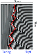
Pattern formation is studied numerically for a reactive microemulsion when two parts of the system with different droplet fractions are initially put into contact. We analyze the resulting dynamics when the volume droplet fraction readjusts by diffusion. When both parts initially sustain Turing patterns, the whole system readjusts its wavelength to the one that corresponds to the mean droplet fraction. Similarly, when both subsystems initially display bulk oscillations, the system readjusts its temporal frequency to that of the mean droplet fraction. More surprisingly, when one of the subsystems shows Turing patterns, and the other bulk oscillations, there is a back and forth invasion of domains, the final pattern corresponding to the one of the mean droplet fraction.

---

1 Introduction

Pattern formation is essentially the interaction of dynamical units through space. It is of importance in several different disciplines such as fluid dynamics, biology, and chemistry just to mention a few.¹ Patterns can be broadly classified in three classes: (i) patterns uniform in space but changing in time, like periodic oscillations, (ii) patterns uniformly distributed in space but stationary in time and (iii) patterns that change both in space and time, like traveling waves. For reaction–diffusion systems, the simplest cases for these patterns occur through different bifurcations for each pattern, and for (i) the stability of the system changes from stable to unstable generating limit cycle oscillations, in what is known as a Hopf bifurcation.¹ For (ii) the system changes stability due to diffusion. Alan Turing described the conditions for this bifurcation as activator–inhibitor dynamics in which the inhibitor diffuses faster than the activator, leading to patterns with a well-defined wavelength.² This type of structure is known as a Turing pattern, and the bifurcation leading to it as a Turing bifurcation. While patterns in the categories (i) and (ii) can be obtained in two-variable systems, for patterns in (iii), at least three variables are needed as well as differential diffusion, and this instability is known as wave instability.²

The interaction of different forms of patterns (or their respective instabilities) extends the wealth of dynamics that can be observed. For instance the interaction of Turing and Hopf bifurcations can produce mixed states such as oscillatory Turing patterns or the coexistence of stable local domains supporting different dynamics but also more complex structures such as spatiotemporal chaos.^1,3–5 Even the transition from one type of pattern to another due to consumption of reactants can produce interesting effects such as wavelength halving between standing and traveling waves⁶ or Turing patterns oscillating in space.⁷ All previous examples consider the interaction of spatial and time breaking symmetries occurring simultaneously through the entire reactor. However, an interesting open question is what kind of dynamics will arise if we adjoin two spatially extended systems, in such a way that the interplay between instabilities will be locally defined and ruled by the Fickian diffusion processes. Experiments putting into contact active media have been recently reported where the reagents of the chemical oscillator, the Belousov–Zhabotinsky reaction, have been initially separated into two adjoined parts.^8,9 Therefore, none of the systems alone are active or can produce patterns, with the pattern formation initially limited to the contact line between them, and the evolving spatio-temporal dynamics dependent on the excitability of the reaction.⁸ Additionally, in the case where systems are put in contact in a gravity field, the emerging dynamics may modulate the hydrodynamic patterns creating an intriguing pulsatile chemo-hydrodynamic coupling.⁹

Our aim in this paper is to understand the resulting dynamics that arise due to the interaction of two active compartments. To do so we use a model^10–12 that describes pattern formation in a chemical system able to display the variety of patterns previously described: the Belousov–Zhabotinsky reaction encapsulated in a water-in-oil microemulsion (BZ-AOT).^13,14 For the BZ-AOT system, the difference in diffusion coefficients happens as there are intermediates of the reaction that can diffuse through the oil phase (diffusing as a single molecule), whereas other intermediates are only soluble in water, so that diffusion occurs as a whole droplet (hence, diffusing slowly).¹³ Once the key processes take place in confinement, the amount of reactive volume entrapped in these nanocompartments is able to modify the kinetics of the reactions and, therefore, the resulting patterns. We show numerically that when two extended BZ-AOT systems containing the same initial chemical conditions are put into contact, the jump in the concentration of the droplets (where the reagents are confined) represents an extraordinary tool to provide new spatio-temporal dynamics. In the next section (Section 2) we describe the model as well as introduce a further variable corresponding to the droplet fraction, in order to couple the two subsystems. In Section 3 we show and discuss the results of the coupled systems: interacting Turing (or Hopf) instabilities give rise to an homogeneous averaged wavelength (or period of oscillation) while the change from Turing patterns to waves or vice versa occurs via back and forth ‘invasion’ of the domains rather than a front that separates the domains moving in one direction. The last section (Section 4) is devoted to the conclusions, with an emphasis on the relation of our findings to possible experiments using the Belousov–Zhabotinsky reaction immersed in a microemulsion.

2 The model

Alonso and coworkers have developed a numerical model for chemical reactions in a water-in-oil microemulsion droplets system that reads:¹²

∂_tu = ϕ(au − αu³ − bv − cw) + ∇(D_e(ϕ)∇u) (1)

∂_tv = ϕε₁(u − v) + ∇(D_e(ϕ)∇v) (2)

∂_tw = ϕε₂(u − w) + ∇(D_w∇w) (3)

This extension of the FitzHugh–Nagumo model has one activator (u) and two inhibitors (v and w) where a, b, c, ε₁, ε₂ and α are the reaction terms and ϕ is the volume droplet fraction, a parameter that accounts for the droplet concentration. Note that the kinetics depend on ϕ, so when few droplets are immersed in the oil, the reaction is slow, while it becomes faster as the droplet fraction increases. Also, the diffusion coefficient for w (D_w) is constant and relatively fast (in comparison with the diffusion of u and v) so that w represents an inhibitor that can diffuse through the oil phase. In contrast, as u and v are assumed to stay inside the droplets, the effective diffusion coefficients for u and v depend on the droplet fraction as:^10–12

This equation takes into account the diffusion coefficients of the droplets (D_d) and the chemicals inside the droplets (D_i). Furthermore, it reproduces the value for the percolation threshold, i.e. the value of ϕ above which the droplets aggregate forming clusters.

The one-dimensional results obtained with this model can be summarized in a phase diagram spanned by the volume droplet fraction ϕ and the autocatalytic reaction rate a, two parameters feasible to tune from an experimental point of view and that complement the characterization done by Alonso et al.¹² A summary of the patterns obtained by keeping b = 3; c = 3.5; α = 4/3; ε₁ = 1; ε₁ = 6; D_d = 0.01 and D_i = 2 is presented in Fig. 1a. The choice of these values for the reaction terms was made to allow the system to display different dynamics by just tuning the volume droplet fraction. Representative patterns obtained at a = 4.5 are presented in Fig. 1b–d along with the corresponding dispersion curves (top). The blue (continuous) line represents the real part and the red (dashed) line the imaginary part of the eigenvalues obtained by means of a linear stability analysis. By increasing the volume fraction for a = 4.5 the system exhibits different dynamics, going from Turing patterns (Fig. 1b, ϕ = 0.5) to chaos (Fig. 1c, ϕ = 0.53) and oscillations (Fig. 1d, ϕ = 0.56). The type of chaos seen in the Alonso–John–Bär model corresponds to alternation in both space and time of oscillations and Turing patterns. Hence it is some type of spatiotemporal intermittency, but rather than alternating attractors from different steady states, which is the most common type of spatiotemporal intermittency,¹⁵ it alternates different attractors from a single steady state. In reaction–diffusion systems, the Gray–Scott model is the prototypical example of spatiotemporal intermittency (see for example ref. 16).

Fig. 1 (a) Phase diagram and (b–d) representative 1D patterns obtained with a = 4.5; b = 3; c = 3.5; α = 4/3; ε₁ = 1; ε₁ = 6; D_d = 0.01 and D_i = 2 in an one-dimensional homogeneous system. In (a) S corresponds to a stable steady state, T-W to a mixture of Turing patterns and waves, T corresponds to Turing patterns, W-BO to waves or bulk oscillations and C to a chaotic intermittent state of Turing patterns and waves.

2.1 Two-compartment model

In the following sections we will study the dynamic behavior of a system composed of two adjoined subsystems, each one with a spatially homogenous volume droplet fraction ϕ but with different values (ϕ(0 : L_x, 0 : L_y) = ϕ₁, ϕ(L_x : 2L_x, 0 : L_y) = ϕ₂, L_x,y being the dimensions of each subsystem), as sketched in Fig. 2. We assume that the droplet fraction jump relaxes as a diffusion process, in which the diffusion coefficient D_ϕ is set equal to D_w. The complete model thus becomes:

∂_tu = ϕ(au − αu³ − bv − cw) + ∇(D_e(ϕ)∇u) (5)

∂_tv = ϕε₁(u − v) + ∇(D_e(ϕ)∇v) (6)

∂_tw = ϕε₂(u − w) + ∇(D_w∇w) (7)

∂_tϕ = ∇(D_ϕ∇ϕ) (8)

Fig. 2 Schematic showing the numerical setup used in the results section and the spatial distribution of the volume droplet fraction.

We integrate the equations using a fully explicit Euler method with a three point approximation with a spatial step of 0.05 s.u. (spatial units) and a temporal step size of 0.001 t.u. (time units) for 1D simulations and a three level DuFort–Frankel method with a spatial step of 0.1 s.u. and temporal step of 0.001 t.u. for 2D simulations. We employ no-flux boundary conditions and positive random initial conditions with amplitude of 0.1 over the (u₀ = 0, v₀ = 0, w₀ = 0) state.

3 Results

Our case of study will be the spatio-temporal dynamics arising from the interaction between two chemical extended subsystems (i = 1, 2) described by the numerical model explained in Section 2. We consider the particular scenario where the subsystems are chemically identical (same a, b, c, α, ε₁ and ε₂ parameters) but containing different droplet concentration (ϕ₁ and ϕ₂). The initial conditions are imposed such that both subsystems are in touch with an initial jump in the volume droplet fraction (Δϕ = ϕ₁ − ϕ₂) along the horizontal axis.

We can summarize the different dynamics through the tunable volume fractions ϕ₁ and ϕ₂ or by using a phase diagram in terms of the initial jump Δϕ and the average volume fraction [small phi, Greek, macron] = (ϕ₁ + ϕ₂)/2 (that corresponds to the homogeneous value once the volume fraction homogenizes throughout space). In these parametric phase diagrams (see Fig. 3) we have inserted a blue region to guide the reader to the location of the chaotic intermittent state previously described in Fig. 1. Our numerical results differentiate four different regimes that will be detailed hereunder. Note that our simulations were carried out by considering ϕ₂ ≥ ϕ₁ and that the four different domains can be symmetrically found above the ϕ₁ = ϕ₂ curve (red line in Fig. 3b).

Fig. 3 Parametric phase diagrams in terms of: (a) the initial volume fraction droplet jump (Δϕ) and the average ([small phi, Greek, macron]) between two spatially adjoined systems and (b) the initial volume droplet fractions ϕ₁ and ϕ₂ summarizing the different spatio-temporal dynamics: Turing–Turing interaction (I), Turing invading Hopf back-and-forth (II), Hopf invading Turing back-and-forth (III) and Hopf–Hopf interaction (IV). The blue domain indicates the chaotic intermittent state obtained for a homogeneous single system.

3.1 Interaction between subsystems supporting Turing instability (case I)

The first case of study is when both subsystems display Turing structures although with distinct characteristic wavelength (see Fig. 4 with the corresponding ϕ spatial distribution at the bottom). This discrepancy is due to the different volume fraction ϕ initially imposed in each subsystem, a parameter that rules the reaction terms of the model as explained in the previous section. The larger the volume fraction in the subsystem the greater the wavelength of the patterns.¹²

Fig. 4 Two snapshots of interacting subsystems developing 2D Turing patterns at different initial volume fraction (top) alongside the corresponding spatial distribution of volume fractions (bottom); ϕ₁ = 0.4 and ϕ₂ = 0.5 (a) at 51 time units and (b) at 20 000 time units. Computational domain size: 200 × 200 space units. Bottom: volume fraction profiles at the initial time (red dashed line) and at the snapshot given time (blue line).

Fig. 4a shows the developed Turing structures after imposing an initial jump in the volume fraction (red dashed line in Fig. 4a bottom). Note that the system requires time to develop the patterns, so when the patterns appear the diffusion processes have already smoothed the curve of ϕ (blue line in Fig. 4a bottom). As time evolves, Turing wavelengths rearrange due to the changes in the spatial profile of the volume fraction, the subsystem with higher ϕ being the one starting sooner to readjust the Turing patterns. This faster readjustment may be explained by the fact that within the model, the kinetics are controlled by ϕ, so with the higher ϕ, the higher the velocities of the reaction.

The final stage is reached once the volume fraction is constant along the entire system, exhibiting an homogeneous Turing wavelength (Fig. 4b). This final wavelength corresponds to the expected value for a system with [small phi, Greek, macron] as observed in the volume fraction profile in Fig. 4b bottom (blue line). The competition of Turing instabilities has been observed even when the subsystem with the larger volume fraction value supports Hopf instability (see Fig. 3 where the region I exceeds the blue domain). This can be explained by the fact that once diffusion takes place, the value of ϕ falls into the regime where both Turing and Hopf modes are supported (Fig. 1).

The relaxation of Turing patterns after imposing an initial condition has been studied in different configurations. For example, spots can be arranged as rhombic patterns instead of hexagonal patterns,¹⁷ as long as an allowed wavelength is selected. In striped systems, the imposed stripes will remain if they match an allowed wavelength, otherwise they will rearrange through transverse instabilities such as Eckhaus and zigzag instabilities^18,19 or even by splitting of stripes.¹⁸ In our case, the relaxation of the patterns is smooth as it is the relaxation of the droplet fraction, so no splitting of stripes or zigzagging is observed.

3.2 Back and forth Turing–Hopf invasion (cases II and III)

We now analyze the case when one subsystem supports Turing patterns while the other one features temporal oscillations. When these two zones come in contact, the transient pattern shows a back and forth invasion of domains. This effect can be clearly observed by performing a space–time plot along both subsystems as shown in Fig. 5. The resulting pattern will differ depending on the final value of the volume fraction once it becomes homogenous through space (i.e. [small phi, Greek, macron]). Thus, if [small phi, Greek, macron] < 0.52 Turing structures will gradually invade the other subsystem until finally occupying the entire reactor (Fig. 5a) or, by contrast, if [small phi, Greek, macron] > 0.55 the whole system will end up displaying oscillations (Fig. 5b and c). The back and forth movement is seen in all cases within the range of 0.55 ≥ ϕ ≥ 0.51 (as highlighted in clear color in Fig. 5) which is slightly larger than the range in which spatiotemporal intermittency between Turing and Hopf modes (chaos) is observed in homogenous systems (Fig. 1).

Fig. 5 Space–time plots demonstrating the back and forth invasion between Turing and Hopf modes for different initial volume fractions. (a) ϕ₁ = 0.4 and ϕ₂ = 0.6, (b) ϕ₁ = 0.45 and ϕ₂ = 0.65, (c) ϕ₁ = 0.5 and ϕ₂ = 0.6. Dimensions of space–time plots: 400 space units (horizontal) and 375 time units (downwards). Highlighted in clear color is the region where 0.55 ≥ [small phi, Greek, macron] ≥ 0.51.

When both the Turing and the Hopf instabilities are present in a system, what is most common is that the most stable pattern will invade the whole system, and the front separating the different regimes will move with a constant velocity, or by removing or adding one Turing wavelength. This phenomenon has been observed in experiments with chlorine dioxide–iodine–malonic acid reactions, where Turing patterns invade a steady state domain as either dividing blobs (for spot patterns) or a growing labyrinth,²⁰ the domain of the Turing pattern being circular. This linear growth of one domain invading the other is seen for Turing patterns emerging from bulk oscillations and a pacemaker,^21,22 as well as traveling waves developing from a pacemaker and bulk oscillations.²² A forced linear growth of a domain with imposed temporal frequency can be used to control the morphology of the patterns.²³

Another possibility when both the Turing and Hopf instabilities are present is that a system may display both patterns in different sub-regions of the system (i.e. localized structures), and that the fronts separating these regions stay stationary.^5,24,25 These results are obtained near the codimension two point, where both the Turing and the Hopf instabilities occur at the same point. The stability of the front separating the Turing and Hopf domains is explained by a periodic potential generated by the interaction with a spatially periodic structure and by the difference in free energy gained by invasion of the most stable domain not being able to compensate for the energy required to move the front by one wavelength.⁵ Stationary or pinned fronts have been studied as well for localized Turing patterns over a homogeneous steady state.^26,27

In our case we have intricate spatio-temporal dynamics different to those previously described. To help the reader understand the processes seen in Fig. 5, we show in Fig. 6 and 7 the one-dimensional spatial profiles of the three species (u, v, w) at different times.

Fig. 6 Profiles of three variables u (blue), v (red) and w (green) at different time intervals showing the creation of Turing patterns from oscillations. We have encircled (in dashed red) the birth of a stationary structure coming from the wave labelled with a black arrow; the gray arrows in the top and bottom figures indicate the same wave while the black arrow indicates the upcoming one. This step creates a bigger Turing domain. Numerical parameters: a = 5.3; b = 3; c = 3.5; α = 4/3; ε₁ = 1; ε₁ = 6; D_d = 0.01; D_i = 2; ϕ₁ = 0.5; ϕ₁ = 0.6.

Fig. 7 Profiles of three variables u (blue), v (red) and w (green) at different time intervals showing the transformation of stationary Turing patterns into waves (encircled). They collide with the waves coming from the opposite direction (see arrows). This mechanism gives way to a reduction of Turing domain. Numeric parameters: a = 5.3; b = 3; c = 3.5; α = 4/3; ε₁ = 1; ε₁ = 6; D_d = 0.01; D_i = 2; ϕ₁ = 0.5; ϕ₂ = 0.6.

On the one hand, each bulk oscillation slows down around the contact line producing a stationary structure (Fig. 6) a certain distance ahead of the Turing patterns. This process, repeated for several cycles, leads to a bigger domain supporting Turing structures. Subsequently, on the other hand, the last stationary structure created turns into a wave once a bulk oscillation is approaching and they annihilate each other (Fig. 7). In contrast with the Turing structures where the maximum of all species (u, v, w) are perfectly aligned, the process of giving motion to the stationary structures is associated with a spatial translocation of the activator (u, blue line in Fig. 7) over the inhibitors (v, w, red and green lines respectively in Fig. 7). As can be observed in the encircled case, the activator goes a short distance ahead in the direction of motion exactly as in the wave propagating in the opposite direction. Contrary to the previous scenario, the reiteration of this process leads to a greater region sustaining oscillations. Both different cases alternate in time, giving rise to a back and forth invasion between Turing and Hopf modes. We want to remark that localized moving patterns with similar asymmetry in the profiles of activator and inhibitors have been previously reported in reaction–diffusion systems with long range inhibition and global coupling.²⁸

For the occurrence of spatiotemporal intermittency, the existence of two different attractors is a necessary but not sufficient condition. There must be a way in which these different states are connected. In the Gray–Scott model, if two neighboring sites are in different attractors, the one corresponding to the limit cycle will induce the one in the steady state to jump out of its attractor. The connection from the remains of the limit cycle to the stable steady state occurs when the unstable state separating the two different attractors becomes part of the limit cycle (what is known as the Andronov homoclinic bifurcation¹⁵). What controls whether the Turing domain grows or shrinks is the wavelength of the pattern and ϕ. If the wavelength is stable for the corresponding local ϕ, the incoming wave will create a new Turing spot. However, as the local ϕ changes (increases), the existing Turing wavelength is too short, and in order to readjust, the spot at the edges has to move towards the right. To do so the spot behaves, as we have seen, as a wave so that it annihilates with the incoming wave. In conclusion, what is important for the back and forth invasion is the dependence of the Turing wavelength with ϕ, so for a system with a small dependence of the wavelength on ϕ, we would not expect this back and forth invasion.

The use of random initial conditions does not have a noticeable effect on patterns when the starting conditions are Turing–Turing interactions or Hopf–Hopf interactions. However, for the Turing–Hopf interaction, the movement of the front separating the domains changes from simulations to simulation but always remaining within the range of 0.55 ≥ ϕ ≥ 0.51. This sensitivity towards initial conditions comes from the chaotic nature of the intermittent state.¹²

3.3 Interaction between subsystems supporting Hopf instability (case IV)

For large volume fraction values (ϕ ≥ 0.55) both subsystems exhibit temporal oscillations. Fig. 8c shows, for early times, the Fourier transforms associated to three different locations in the system shown in Fig. 8a: in the domain with initial lower volume fraction (ϕ = 0.55, blue curve), higher (ϕ = 0.75, green curve) and in the contact line between both (red line). During this initial stage we observe that the oscillations are made quicker by increasing the volume fraction. This trend can be confirmed by performing a linear stability of the model and analyzing the dependence of the imaginary part of the eigenvalue on the volume fraction (see ref. 12 for details).

Fig. 8 Space–time plots at the beginning (a) and at the end (b) of a 5000 t. u. simulations. The size of the space–time plots is 100 s. u. (horizontal) × 100 t. u. (downwards). (c) and (d) are the corresponding Fourier transforms, the color corresponding to the lines marked in (a) and (b).

When two subsystems displaying oscillations with different periodicity interact, the overall system tries to readjust the frequency of oscillations as diffusion takes over. To do so, the faster oscillations slow down around the contact region, propagating as a traveling wave through the other domain (see Fig. 8a). Once the volume fraction becomes spatially homogeneous, the entire system exhibits an unique periodicity as confirmed by the Fourier analysis at different spatial locations (Fig. 8d). The final frequency is the average of the values initially obtained for ϕ₁ and ϕ₂ (blue and red line in Fig. 8a, respectively) and corresponds to the expected value for a system with a volume fraction [small phi, Greek, macron].

It is known that when oscillators of different frequencies are coupled, the source of highest frequency dominates the whole system.²⁹ In our system, the dominating frequency also changes with time as the volume fraction changes. At the beginning of the simulations, we observe that, sometimes, the wave from the right part of the system is unable to propagate into the left part of the system creating a defect. This kind of defect, generated by a steep gradient in the volume fraction, leads to the formation of spiral waves as demonstrated by the Belousov–Zhabotinsky reaction with the addition of a zwitterionic surfactant.³⁰

4 Conclusion

We have observed three different spatio-temporal dynamics depending on the initial values of volume fractions, the tunable parameter in this work. Thus, a system initially exhibiting two arrangements of Turing patterns with different wavelengths will readjust their spatial gaps until becoming homogeneous at an intermediate value. In the same way, when the system supports two different Hopf modes, the resulting periodicity becomes the mean value of the initial ones. More intriguing and unexpected dynamics arise when the initial jump in volume fraction allows the interaction between Turing and Hopf modes. In this case the transient dynamics gives rise to a back and forth invasion between both instabilities, mainly due to two opposed mechanisms: the formation of Turing structures by “frozen” bulk oscillations and the posterior acceleration of the stationary structures resembling traveling waves. The competition of these two processes lasts for a long time but one of the mechanisms, on average, gains in space until it becomes predominant and homogeneous over the entire system. The value of the average volume fraction is the key factor to determine the resulting dynamics.

Since the Alonso–John–Bär model is developed to simulate patterns for a reaction in a reverse microemulsion, can we think of an experimental confirmation of the phenomena that we observe? The key issue for the back and forth invasion of domains is the existence of the chaotic regime between Turing patterns and oscillations or waves. The existence of localized structures has been used to create a memory device using the Belousov–Zhabotinsky reaction in a reverse microemulsion.³¹ However, under different conditions this system may show spatiotemporal intermittency. For instance, in the chlorine dioxide–iodine–malonic acid reaction, the transition from waves to Turing patterns occurs through the formation of dashed waves, which themselves have a chaotic behavior.³² Dashed waves were first observed in the Belousov–Zhabotinsky reaction in a reverse microemulsion,³³ so this regime may be a good starting point. The possibility to tune one physical parameter (such as the volume fraction) that follows the Fickian laws of diffusion, without changing the chemical concentration of the reagents, represents an unusual way to achieve novel dynamics. We believe that the use of this methodology in experimental set-ups will constitute a good tool to provide more light into the field of self-organizing structures.

Our system eventually equilibrates, but while it is out of equilibrium the medium can influence the dynamical behavior occurring within itself. We can speculate that if a microemulsion is used in chemical synthesis, and that the properties of the media are changing, these changing properties can be used to control the outcome of the reaction. One example is again the dashed waves in the Belousov–Zhabotinsky reaction in a reverse microemulsion: These dashed waves were observed when the distribution of the droplet size is bimodal.³³ This bimodal distribution is a transient process, however when such distribution is stabilized, the lifetime of the dashed waves is greatly increased.³⁴

Acknowledgements

I. B. acknowledges funding from ARC CONVINCE and J. C.-L. financial support from F.R.S.-FNRS. The authors would like to thank Prof. A. De Wit for helpful discussions.

References

1. M. C. Cross and P. C. Hohenberg, Rev. Mod. Phys., 1993, 65, 851–1112.
2. A. M. Turing, Philos. Trans. R. Soc. London, Ser. B, 1952, 237, 37–72.
3. L. Yang, M. Dolnik, A. M. Zhabotinsky and I. R. Epstein, J. Chem. Phys., 2002, 117, 7259–7265.
4. A. De Wit, G. Dewel and P. Borckmans, Phys. Rev. E: Stat. Phys., Plasmas, Fluids, Relat. Interdiscip. Top., 1993, 48, R4191–R4194.
5. A. De Wit, D. Lima, G. Dewel and P. Borckmans, Phys. Rev. E: Stat. Phys., Plasmas, Fluids, Relat. Interdiscip. Top., 1996, 54, 261–271.
6. A. Kaminaga, V. K. Vanag and I. R. Epstein, Phys. Rev. Lett., 2005, 95, 058302.
7. J. Carballido-Landeira and A. P. Muñuzuri, Langmuir, 2015, 31, 3021–3026.
8. M. A. Budroni, L. Lemaigre, D. M. Escala, A. Perez-Muñuzuri and A. De Wit, J. Phys. Chem. A, 2016, 120, 851–860.
9. D. M. Escala, M. A. Budroni, J. Carballido-Landeira, A. De Wit and A. P. Muñuzuri, J. Phys. Chem. Lett., 2014, 5, 413–418.
10. D. Bedeaux and R. Kapral, J. Chem. Phys., 1983, 79, 1783.
11. S. Alonso, R. Kapral and M. Bär, Phys. Rev. Lett., 2009, 102, 238302.
12. S. Alonso, K. John and M. Bär, J. Chem. Phys., 2011, 134, 094117.
13. V. K. Vanag and I. R. Epstein, Phys. Rev. Lett., 2001, 87, 228301.
14. J. Carballido-Landeira, P. Taboada and A. P. Muñuzuri, Phys. Chem. Chem. Phys., 2011, 13, 4596–4599.
15. M. Argentina and P. Coullet, Phys. A, 1998, 257, 45–60.
16. R. Wackerbauer and K. Showalter, Phys. Rev. Lett., 2003, 91, 174103.
17. G. H. Gunaratne, Q. Ouyang and H. L. Swinney, Phys. Rev. E: Stat. Phys., Plasmas, Fluids, Relat. Interdiscip. Top., 1994, 50, 2802–2820.
18. I. Berenstein, M. Dolnik, A. M. Zhabotinsky and I. R. Epstein, J. Phys. Chem. A, 2003, 107, 4428–4435.
19. B. Peña, C. Pérez-García, A. Sanz-Anchelergues, D. G. Míguez and A. P. Muñuzuri, Phys. Rev. E: Stat., Nonlinear, Soft Matter Phys., 2003, 68, 056206.
20. P. W. Davies, P. Blanchedeau, E. Dulos and P. De Kepper, J. Phys. Chem. A, 1998, 102, 8236–8244.
21. S. Sen, P. Ghosh, S. S. Riaz and D. S. Ray, Phys. Rev. E: Stat., Nonlinear, Soft Matter Phys., 2010, 81, 017101.
22. I. Berenstein, Chaos, 2012, 22, 023112.
23. M. Kaern, D. G. Míguez, A. P. Muñuzuri and M. Menzinger, Biophys. Chem., 2004, 110, 231–238.
24. J.-J. Perraud, A. De Wit, E. Dulos, P. De Kepper, G. Dewel and P. Borckmans, Phys. Rev. Lett., 1993, 71, 1272–1275.
25. M. Meixner, A. De Wit, S. Bose and E. Schöll, Phys. Rev. E: Stat. Phys., Plasmas, Fluids, Relat. Interdiscip. Top., 1997, 55, 6690–6697.
26. O. Jensen, V. Pannbacker, G. Dewel and P. Borckmans, Phys. Lett. A, 1993, 179, 91–96.
27. O. Jensen, V. O. Pannbacker, E. Mosekilde, G. Dewel and P. Borckmans, Phys. Rev. E: Stat. Phys., Plasmas, Fluids, Relat. Interdiscip. Top., 1994, 50, 736–749.
28. K. Krischer and A. Mikhailov, Phys. Rev. Lett., 1994, 73, 3165–3168.
29. O.-U. Kheowan, E. Mihaliuk, B. Blasius, I. Sendiña Nadal and K. Showalter, Phys. Rev. Lett., 2007, 98, 074101.
30. M. A. Budroni and F. Rossi, J. Phys. Chem. C, 2015, 119, 9411–9417.
31. A. Kaminaga, V. K. Vanag and I. R. Epstein, Angew. Chem., Int. Ed., 2006, 45, 3087–3089.
32. L. Yang, I. Berenstein and I. R. Epstein, Phys. Rev. Lett., 2005, 95, 038303.
33. V. K. Vanag and I. R. Epstein, Proc. Natl. Acad. Sci., 2003, 100, 14635–14638.
34. J. Carballido-Landeira, I. Berenstein, P. Taboada, V. Mosquera, V. K. Vanag, I. R. Epstein, V. Pérez-Villar and A. P. Muñuzuri, Phys. Chem. Chem. Phys., 2008, 10, 1094–1096.

---

Footnote

† These authors contributed equally to this work.

---