Techno-economic analysis of tandem photovoltaic systems

Abstract

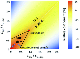
Tandem solar cells offer the potential of conversion efficiencies exceeding those of single-junction solar cells, but also incur higher fabrication costs. The question arises under which conditions a tandem solar cell becomes economically preferable to both of the single-junction sub-cells it comprises. We present an analysis based on cost and efficiency relations to answer this question for a double-junction tandem solar cell. We find that combining two ideally band-gap-matched single-junction solar cell technologies into a tandem should be a “marriage of equals”: the sub cells should be produced at similar $ per W costs, both sub cells should have similar efficiencies when operated independently, and the costs to turn both cells into a system should be similar. We discuss examples of different hypothetical and actual tandem solar cell technologies and show the intricacies of imbalances in the mentioned factors. We find that tandem-solar-cell-based PV power stations for existing solar-cell technologies offer the potential to reduce the levelized cost of electricity (LCOE), provided suitable top cells are developed.

---

1. Introduction

“Efficiency” is the technical variable that most strongly influences the cost of electricity provided by solar cell modules and systems.¹ With established technologies like Si^2–4 and GaAs^4–6 approaching their practical efficiency limits, non-concentrating tandem solar cell^7–10 technology has gained renewed interest. Tandem solar cells offer a path to increase efficiencies beyond the Shockley–Queisser limit¹¹ by stacking multiple junctions made from different absorber materials, thus reducing thermalization losses.¹² Tandem technology is appealing because it can leverage well-established technologies with AM1.5 efficiencies >20%. Resulting tandem efficiencies exceed single-junction efficiencies by several percent absolute. Highest efficiencies were achieved with III–V materials;^13–15 recently reaching 29.8% with GaInP on Si.¹⁶ Pathways to practical efficiencies exceeding 33% (ref. 17) exist. Notable are also results for hybrid organic lead halide perovskites^18,19 on silicon tandem solar cells²⁰ that offer a potential path to low-cost manufacturing and have recently exceeded 20% efficiency.²¹ Other thin-film technologies like CdTe^22,23 and CIGS²⁴ also offer low-cost and high efficiency potential.

A tandem solar cell is economically viable if and only if the cost of the electric power provided by the tandem is lower than that of either the top or bottom single-junction cell operating independently. At first glance, tandems require only a “small” additional areal cost associated with a few thin-film layers to achieve the aforementioned efficiency gain. However, tandems have hitherto failed to gain market traction, because the benefits of efficiency improvements to date have not exceeded the cost of the additional fabrication steps, balance of systems, and power electronics.

In this work, we conduct a techno-economic analysis with parametric cost relations, to identify the circumstances under which tandems are economically preferable to single-junction constituent devices. Cost modelling is a valuable method to determine innovation pathways to achieve cost reductions for PV electricity.^1,25–31 We use a bottom up cost-model and the minimum sustainable price (MSP) methodology to calculate $ per W, as formulated by Doug Powell and Alan Goodrich¹ for silicon and by Sin Cheng Siah³² for CdTe. To calculate levelized cost of electricity (LCOE), we use the System Advisor Model (SAM) from the National Renewable Energy Laboratory.³³

Once baseline models are established, we explore a wider techno-economic parameter space by developing parametric cost relations, thus identifying under which circumstances it is economically beneficial to combine two single-junction solar cell technologies at AM1.5 conditions into a tandem. Our simplified parametric cost relation requires only two inputs: the ratio of solar cell to system related costs, and the efficiency of the three solar cells (one tandem and two single-junction devices). Definition of the cost relations is formulated, and an efficiency calculation for tandem solar cells is described in the “Methodology” section. The cost breakdown for PV modules and PV installations is discussed in the section entitled “Breakdown of system costs”. We then describe the impact of different technical and economic parameters on the cost-effectiveness of tandems and show the negative effects of imbalances for these parameters. We find that tandems make economic sense only when three conditions are satisfied simultaneously: (1) the band-gaps are well matched to enable a high efficiency potential, (2) the areal manufacturing costs ($ per m²) of top and bottom single-junction devices are similar, and (3) both sub-cells have a similar efficiency when operated independently (marriage of equals). We conclude with a recommendation for future research, including the need for a wider range of low-cost ($ per m²), high-efficiency, low-capex, and highly reliable absorbers with band-gaps in the 1.4–1.9 eV range.

2. Methodology

The presented methodology aspires to relate the cost of energy for a tandem solar cell with the cost of energy of the two single-junction solar cells it comprises. For this purpose we estimate (i) the cost of a tandem solar cell system from the cost of the two comprising single-junction solar cell systems, and (ii) the efficiency of a tandem solar cell from the efficiencies of the two single-junction solar cells it is made of.

2.1 Relation of single-junction solar cell and tandem solar cell system costs

First we need to define the term “PV system”. In the context of this analysis, the term PV system is used in a broad sense and refers to any arrangement of components that may include solar cells, a supporting structure, electronics to convert DC electricity into AC, and other system costs. We intentionally define the term “PV system” broadly, so it comprises both PV modules and PV power stations, which serve as exemplary systems in our analysis.

For any such system, it is possible to break down the system costs C_sys into one part that is associated with the cost of making the solar cells C_cell and one part associated with the cost of making the supporting structure C_str. Fig. 1 shows a schematic sketch of this approach, with more detailed explanations in Sections 3.1 and 3.3.

Fig. 1 Schematic sketch of the definition for a PV system used in this study.

For a single-junction (sj) solar cell the break down is then given by

C_sys,sj = C_cell + C_str,sj. (1)

In the following section, we discuss how these values are determined for a PV module and a PV power station. For a double junction (dj) tandem solar cell PV system, costs can be split up in an analogous way

C_sys,tan = C_cell,top + C_cell,bot + C_str,tan, (2)

where C_cell,top (C_cell,bot) is the cost to fabricate the top (bottom) junction. In the following, we will abbreviate this term as C_top (C_bot). In general, the breakdown defined in (1) and (2) is ambiguous as some elements could be counted as part of the cell or part of the structure. In the present analysis, the breakdown will be made such that the cost for fabricating a junction of a certain material is the same for the single-junction- and the tandem solar-cell fabrication processes. In this way, the breakdown becomes unique and the generality of the presented results is not affected. Differences between the single-junction and the tandem fabrication process are now summarized in the costs of the supporting structure C_str. For example, if a tunnel junction³⁴ is required, the additional cost of the tunnel junction is embedded in C_str.

Depending on the specifics of the fabrication process, C_str,sj could differ significantly from C_str,tan. This is particularly the case for PV modules and for highly integrated tandem fabrication processes. For PV power stations, the differences will be smaller, as many of the components will be required regardless of the specifics of the solar cell. In the following, we will assume whichever structure cost of the two single-junction solar cells is higher as an approximation for the structure cost of the tandem.

C_str,tan ≈ Max[C_str,top, C_str,bot]. (3)

This approximation can be turned into an equation by introducing a factor ΔC,

C_str,tan = Max[C_str,top, C_str,bot] + ΔC. (4)

The factor ΔC summarizes all differences between the single-junction and the tandem fabrication process. We discuss these differences and what values ΔC can take later in this section.

Finally, we define the relative cost-benefit function as

where C_sys,top and C_sys,bot are the costs of making PV systems using only single-junction top or bottom cell respectively, P_top and P_bot are the powers generated by PV systems made from single-junction top or bottom cell, and P_tan is the power generated by the tandem PV system. The function R is unitless and its entries are deliberately ambiguous, as the analysis encompasses different types of PV systems. While C is always in unit of $, P depends on the type of system investigated. For a PV module, P is power in units of watts, whereas for a PV power station, P represents work in units of kilowatt hours. Both quantities are ultimately calculated from the efficiency of the corresponding solar cell, but the later involves assumptions that ultimately lead to energy-yield calculations.³⁵

R is positive if the cost per output is lower for a given tandem PV system than for each of the single-junction PV systems it comprises – hence, if the tandem PV system is economically preferable. The value of R states how much the cost per output of the tandem PV system is lower (in percent) than the cost per output of the less expensive single-junction PV system. The term “output” can refer to power or work, depending on the system considered.

2.2 Relation of single-junction solar cell and tandem solar cell efficiencies

In a second step, we need to relate the power or work generated or done by the tandem solar cell PV system to that of the single-junction solar cells it comprises. Work and power can both be calculated from the solar cell power-conversion efficiency. As a first-order approximation, we use solar-cell efficiencies as proxies for power and work. Consequently, we need to relate the efficiencies of the tandem solar cell η_tan and the efficiencies of the two single-junction solar cells η_top and η_bot. Note that when mentioning a single-junction solar cell efficiency, we always refer to the efficiency generated by this solar cell on its own and under standard testing conditions.

The radiative efficiency limit of a single-junction solar cell η_SQ was determined by Shockley and Queisser.¹¹ In this limit, the efficiency is completely determined by the band-gap E_g of the material used. The limiting efficiency of a double-junction solar cell can be calculated by a modification of this approach⁷ and is completely determined by the band-gaps of the two sub-cells, E_g,top and E_g,bot. The tandem solar cell is, however, not uniquely defined by the two band-gaps. It also depends on how the two sub-cells are integrated. Mainly, there are two possible configurations: a two- and a four-terminal configuration. In the four-terminal configuration, both sub-cells are contacted independently. Efficiencies for top and bottom cell are calculated separately and are added to obtain the tandem efficiency. In the ideal case, all solar photons with energies up to hυ < E_g,top are utilized by the top cell, which is identical to the top cell being operated as a single-junction cell. The bottom cell efficiency is calculated with an altered spectrum, containing all photons with energies E_g,top < hυ < E_g,bot.

In the two-terminal configuration, the sub cells are monolithically integrated and electrically separated by a tunnel junction. The sub-cell with lower current generation limits the current of the tandem device. If the bottom cell is limiting, current generation in the top cell, j_top can be reduced, within limits, by thinning^36,37 or by area adjustment.³⁸ Thus

with j_tan (j_bot) the current generated by the tandem (bottom) solar cell. The voltages generated by the two sub-cells are added to obtain the tandem solar cell efficiency.

The efficiency of a non-ideal single-junction solar cell η_sj can be defined by two parameters: the band-gap of the material used and the fraction f_SQ of the radiative limit at which the solar cell is operating. Thus,

η_sj(E_g, f_SQ) = η_SQ(E_g)f_SQ. (7)

The efficiencies of two non-ideal single-junction solar cells can then be linked to the efficiency of a tandem solar cell. The tandem solar cell efficiency is given as a function of E_g,top, f_SQ,top, E_g,bot and f_SQ,bot. The scaling factors f_SQ,top (f_SQ,bot) provide no freedom of breaking down losses into parts corresponding to current, voltage and fill factor. As different distributions into these parts are possible, the tandem solar cell efficiency is not uniquely given if the single-junction efficiencies are known. Furthermore, the approach does not take into account any additional losses that occur by tandem integration. The used approach can, therefore, only serve as a first-order approximation. The approximation works the better, the closer to the radiative limit the two single-junction cells operate. For a more detailed analysis, a complete device simulation is required.

The broad view presented in this analysis necessarily ignores some aspects that will affect the comparison of single junction and multi junction solar cells. This topic has been discussed in the context of PV LCOE.³⁹ Examples for such factors are differences in the energy yields of single junction and multi-junction solar cells³⁵ and degradation.

2.3 Cost regimes

An example of R(C₁, C₂) is plotted in Fig. 2; we will refer to this type of plot as “cost-regime plot”. Parameters used in the plot are stated in the figure caption. The used parameters do not correspond to any fabricated solar cell system; they were chosen because they represent an ideal example of a tandem solar cell from a cost relation point of view. It will be discussed in the following sections, in what sense this example can be considered ideal. Axes in the cost-regime plot are given as the ratio of solar cell C_cell to supporting structure C_str cost. A ratio of one signifies equal cost shares and corresponds to 50% contribution of each cost to the system cost C_sys.

Fig. 2 Exemplary cost-regime plot. The tandem solar cell comprises a top cell with a band-gap of E_g,top = 1.74 eV, and a single-junction efficiency of η_top = 21.8% (f_SQ,top = 76%). The bottom solar cell (E_g,bot = 1.124 eV) has a single-junction efficiency of η_bot = 21.8% (f_SQ,bot = 64%). The calculated tandem efficiency is η_tan = 32.7% in the four-terminal configuration. The two-terminal efficiency would be η_tan = 32.3%. Structure costs for all three solar cells are equal (C_sys,top = C_sys,bot = C_sys,tan).

The plot in Fig. 2 marks three regimes, separated by the black and white lines. In each regime either of the three solar cell systems, using only the top cell (upper left), using only the bottom (lower right) cell and using the tandem (lower left corner) has the lowest cost per output. The lines mark the conditions under which two of the three solar cell systems have the same cost per output. The triple point marks the condition for which all three solar cell systems are at the same cost per output. In the depicted ideal case the triple point is located at (1, 1).

The white line additionally marks the gradient and the ridge in relative cost-benefit. Approaching the extension of the white line within the tandem regime is, therefore, desirable. From this we draw the first conclusion about under which conditions two solar cells should be combined into a tandem: both solar cells, operated in a system independently, should be at a similar cost per output level.

Another point of interest is the maximum relative cost benefit (MRCB). The MRCB is located numerically by analysing the cost-relations plot. It will later be used to compare impacts of different parameters on the financial competitiveness of the tandem PV system. In Fig. 2, the MRCB is located in the origin. However, this is not generally the case.

3. Breakdown of system costs

As indicated earlier, the term “system” in this work is used in a broad sense. The presented method for analysing cost regimes is valid for any arrangement that includes solar cells and supporting structural components. We will in the following discuss two classes of systems of interest: PV modules and PV power stations. These examples address the economic interest of different trades: module manufacturers for which we will use the MSP as a figure of merit, and PV installers or yieldcos for which we will use the total system costs and LCOE as a figure of merit. As these two system types include different components, also the breakdown of system costs will be different. We will show how such a break down can be made and indicate what values for C_cell/C_str can be expected in each case. Note that the presented analysis uses data for cases within the United States, and numbers would have to be adapted for other locations.

3.1 PV modules

We analyse two PV module fabrication processes: monocrystalline silicon and CdTe, as an example for a thin-film technology. Bottom-up cost analyses for these processes are presented in ref. 1 and 32. Table 1 shows a cost breakdown for these fabrication processes in three categories: feedstock & absorber, absorber to cell and cell to module. Each of those categories can be further broken down into material, labour, electricity, maintenance and capex related costs (not shown). For CdTe we included two examples: one process for a module with frame and one process for a frameless module. C_cell includes feedstock & absorber and absorber to cell costs. C_str includes all cell to module costs. As indicated earlier, we performed the break down such that C_cell would be similar in a tandem fabrication process and all variations are subsumed under C_str. One example for which this issue this has an effect is the glass substrate for the thin-film solar cell. Usually, the glass would be considered part of the absorber to cell process. Here, we consider it as part of the cell to module process. This has two reasons: (i) in a silicon PV module, glass is used as a cover and we wanted the two processes to be as close as possible, and (ii) in a tandem solar cell, one of the cells would be deposited on an existing junction and not on glass. The results of our analysis are summarized in Table 1. The first column for each technology states the fabrication cost, the second column the MSP.

Table 1 Cost breakdown for different single-junction solar cell module technologies

		CdTe single-junction, frameless		CdTe single-junction, with frame		Silicon single junction
		Cost [$ per m^2]	MSP [$ per m^2]	Cost [$ per m^2]	MSP [$ per m^2]	Cost [$ per m^2]	MSP [$ per m^2]
Feedstock & absorber	Ccell	17.98	30.77	17.98	30.77	42.08	56.16
Absorber to cell	Ccell	17.76	26.22	17.76	26.22	27.12	39.64
Cell to module	Cstr	21.43	25.29	25.39	29.93	33.81	42.94
Total		57.16	82.27	61.13	86.92	103.01	138.74
Ccell/Cstr		1.67	2.25	1.41	1.90	2.04	2.23

---

Using this cost breakdown, we can project the costs for a hypothetical tandem fabrication by combining different materials. In Table 2 we show the combination for a hypothetical thin-film on silicon tandem PV module, and a hypothetical frameless thin-film on thin-film tandem PV module. Initially we assume that all processes steps are similar to single junction, i.e., ΔC = 0. The table again states fabrication costs and MSP.

Table 2 Cost breakdown for two hypothetical tandem module technologies

	TF on silicon tandem		TF on TF tandem (frameless)
	Cost [$ per m^2]	MSP [$ per m^2]	Cost [$ per m^2]	MSP [$ per m^2]
Feedstock & absorber (top)	17.98	30.77	17.98	30.77
Absorber to cell (top)	17.76	26.22	17.76	26.22
Feedstock & absorber (bot)	42.08	56.16	17.98	30.77
Absorber to cell (bot)	27.12	39.64	17.76	26.22
Cell to module	33.81	42.94	25.39	25.29
Total	138.76	195.72	92.90	139.25

---

3.2 Discussion of ΔC

In the breakdown shown in Table 2, single-junction and tandem solar cell PV module fabrication processes use the exact same process steps. While feedstock and absorber costs should remain largely unaffected, differences can be anticipated in the absorber to cell process in actual fabrication. These differences will depend on the tandem solar cell architecture. In the following we will give a brief discussion on ΔC for a two-terminal and a four-terminal tandem PV module.

Two-terminal configuration. In the two-terminal configuration, the cell process can be assumed to be highly integrated. The top thin-film solar cell is deposited onto the silicon- or the thin-film bottom cell. The cells are electrically connected by a tunnel junction. Consequently, the rear contact of the top cell and the front contact of the bottom cell become obsolete. We estimate the corresponding savings to be up to 5 $ per m².

While the tunnel junction is an added feature of the tandem solar cell, other features of the single-junction solar cell become also obsolete. Among them is the antireflection (AR) coating of the bottom cell. We hypothesize that the tunnel junction deposition replaces the AR coating deposition and that the tunnel junction can be integrated in fabrication with the front passivation of the bottom cell and the rear passivation of the top cell. As a result, we don't assume any additional cost for the tunnel junction.

A further factor to consider is fabrication yield. As the integrated fabrication process requires more fabrication steps, yield will likely decrease. A decreased yield would result in higher cost. Following the processes described in ref. 1 and 32, a yield reduction of 1% absolute for the tandem PV module was assumed.

Further potential costs could be related to the higher power generated by the tandem solar cell PV module. This could have implications on the modularization process; different wiring or different junction boxes could be required. This is not considered here.

Following the given discussion, we expect ΔC for the 2-terminal configuration to be up to −5 $ per m². This corresponds to 15% of the cell to module costs for a silicon PV module and 23% for a thin-film PV module.

Four-terminal configuration. In the four-terminal configuration, the two sub cells are fabricated and operated independently. We will assume here that they are mechanically stacked. Fabrication procedure and yield remain largely unaffected; though, the four-terminal tandem requires some changes in the design of top and bottom cell.

As the top cell needs a translucent rear contact, the full-area metal contact needs to be replaced by a transparent contact and a rear AR coating. AR coatings can potentially be deposited on both sides of the cell at the same time. The full area metal contact could be replaced by a metal grid. Ensuing costs are marginal and we neglect additional cost for these changes.

Mechanical stacking will, most likely, require an additional polymer layer between the two sub-cells. An air layer is, however, possible. An additional EVA layer would come at an additional cost of 1.8 $ per m².

Potential design changes in the bottom cell include AR coating thickness and junction profile. Foreseeable changes in process costs are small and are ignored here.

Independent contacts for the two sub cells require independent circuitry, an additional junction box and additional cables. We estimate ensuing costs at $7.5 per module (4.6 $ per m²). Integration could reduce this cost and a customized junction box and cable design could be envisioned that includes contacts for both cell types and could reduce this cost factor.

Considering these changes, ΔC for the 4-terminal configuration would be 6.4 $ per m², corresponding to 19% of the cell to module cost for a silicon module and 30% for a (frameless) thin-film module.

Relative changes in the cell to module process correspond directly to changes in MSP. We have plotted the impact of a change in ΔC of ±25% relative on the cost regime in Fig. 3. Note that this analysis was conducted for a specific case and location and that all results are likely to vary as a result of the variation in PV module manufacturing by geography/manufacturer.^40,41

Fig. 3 Effect of a relative change in ΔC on the cost regimes. The black lines border conditions in which the tandem solar cell provides a positive cost benefit. A change in ΔC scales the corresponding area and moves the triple point along the (white) line for equal cost per output of the top and bottom cell.

3.3 PV power stations

The cost breakdown for PV power stations requires a generalization of the approach used for PV modules. The cost of a PV power station includes more cost components than that of a PV module, including costs for PV module, racks, mounting, wiring, land, permits, labor, and inverters. Replacing single-junction solar cells in a PV power station by more efficient tandem solar cells results in the station generating more power. Consequently, all components that scale with a higher power output for a constant area or number of PV panels need to be considered as a part of C_cell. Apart from the solar cells, this includes especially inverters and cables. C_str includes all other components. We used ref. 1 and 32 again for the solar cell and module costs and material published within the solar advisory model (SAM) from ref. 33 to establish C_str and C_cell. As C_str changes with the size of the installation, we have considered three different station sizes for each residential scale and utility scale. Additionally, for each solar cell technology, CdTe and Si, we considered three different efficiencies. These efficiencies will later be used to investigate the impact of different parameters on the cost regimes. The results of the calculations are summarized in Table 3.

Table 3 Cost breakdown for different single-junction solar power stations. The 1 kW residential and the 600 MW utility scale system mark the smallest and largest value in each row

Cell type	η [%]	MSP [$ per W]	Ccell/Cstr
			Residential			Utility
			1 kW	5 kW	13.5 kW	50 MW	186.7 MW	600 MW
CdTe	14.0	0.62	0.077	0.168	0.206	0.313	0.332	0.338
	16.4	0.53	0.069	0.160	0.202	0.319	0.331	0.337
	20.8	0.40	0.059	0.148	0.197	0.308	0.337	0.345
Si	12.2	1.14	0.139	0.283	0.339	0.499	0.524	0.531
	16.4	0.85	0.114	0.260	0.326	0.488	0.521	0.530
	24.7	0.56	0.084	0.224	0.301	0.467	0.514	0.527

---

Comparing Tables 1 and 3, the significant difference between C_cell/C_str for PV modules and power stations becomes clear. Whereas in a PV module this ratio is between 1.4 and 2.3, for power stations the ratio is between 0.06 and 0.5. From this result it can be concluded that, whether a tandem solar cell is economically attractive, will be judged differently by a module manufacturer and a system installer or yieldco. The smaller ratios for power stations show that tandem solar cell technology will become interesting to installers before it will become interesting to manufacturers.

It also becomes obvious that the main share of the cost in a PV power station is not related to solar cells. This has implications on ΔC. It can be argued that fabrication differences between two- and four-terminal solar cells are exhausted at the module level. For example, as cables and inverters scale with power, wiring in four-terminal tandems could be imagined that connects different inverters to different cells. Therefore, most of C_str becomes independent of the solar cell technology and the relative differences become much smaller. We estimated ΔC at ±3% of C_str at the power station level.

4. Impact of different parameters on cost relations

4.1 Impact of different pairings of band-gaps (E_g)

The combination of band-gaps of top and bottom cell determines the limiting efficiency for the tandem solar cell. This limit is different for the two- and four-terminal configuration, as the former requires current matching. We calculated the limiting efficiencies for a range of different band-gap pairs according to the method described in the methodology section for the two- and four-terminal configuration. The results of this calculation are shown in Fig. 4 and are plotted as contour lines. We also calculated which band-gap pairing gives the highest efficiency for a given top cell/bottom cell band-gap (blue dotted line). For each band-gap pairing, we calculated the MRCB, which is represented by the color code. Finally, we calculated the band-gap pairing that gives the highest MRCB for a given bottom/top cell band-gap (black and red line, respectively). Generally, the band-gap pairings that result in the highest efficiency also result in the highest MRCB. This is strictly true for the two-terminal configuration. For the four-terminal configuration, there is an ambiguity for small bottom-cell band-gaps (E_g,bot < 1 eV). The result depends on whether in the calculation the top- or the bottom-cell band-gap is fixed.

Fig. 4 Maximum relative cost benefit as a function of top cell band-gap E_g,top and bottom cell band-gap E_g,bot for the four-terminal (a) and two-terminal (b) configuration. The contours show the limiting efficiencies for the corresponding band-gap combination. The blue dotted line represents the band-gap pairing with the highest efficiency for a given E_g,top, E_g,bot. The black line represents the band-gap pairing with the highest relative cost benefit for a given E_g,bot. For the four-terminal tandem, we also show the band-gap pairing with the highest relative cost benefit for a given E_g,top (red line).

The reason for the peculiar behavior of the four-terminal configuration lies in the relative nature of the metric. A single-junction solar cell with either a very small or a very large band-gap generates a very small efficiency on its own. In the four-terminal configuration, the efficiencies of a top cell with a large band-gap and a bottom cell with a small band-gap nearly add up. The relative cost benefit compared to either of the single-junction solar cells is then very large, but the absolute price per output is very high, so that these combinations are not actually desirable. To avoid these solutions, it is necessary to look at both, the E_g,top that results in the highest MRCB for a fixed E_g,bot (black line) and the E_g,bot that results in the highest MRCB for a fixed E_g,top (red line).

To illustrate the effect of different band-gap pairings on cost regimes, we compare a close to ideal band-gap pairing on silicon (E_g,bot = 1.124 eV, E_g,top = 1.74 eV) to a non-ideal one (E_g,bot = 1.124 eV, E_g,top = 1.42 eV). The results are shown in Fig. 5. For the close to ideal band-gap pairing (Fig. 5a), we used a top cell efficiency of η_top = 20.8%, corresponding to a value of f_SQ,top = 72%. This efficiency was chosen with the current record efficiency for GaInP⁴² in mind. The band-gap of GaInP can be tuned by a variation of In and P content. The current record efficiencies were achieved with a material that had a slightly higher band-gap (1.81 eV). A silicon solar cell with the same cell quality (f_SQ,bot = 72%) is at η_bot = 24.7%, which is about 1% below world record.⁴³ The calculated tandem solar cell efficiency for this combination would be η_tan = 33.2% (four terminal) or η_tan = 32.6% (two terminal).

Fig. 5 Illustration of the impact of ideal and non-ideal band-gap combination on the cost regimes. A close to ideal band-gap pairing is shown on the left (a), a non-ideal band-gap pairing on the right (b). The blue line at the top of each graph represents the C_cell/C_str value for a silicon PV module (Table 1), the blue band at the bottom represents the range of C_cell/C_str values for different silicon PV power stations (compare Table 3). The lower boundary corresponds to a small residential system, the upper boundary to a large utility scale system. $ per W values show at what MSP levels the module would be.

The non-ideal case corresponds to a GaAs on Si tandem solar cell.³⁵ GaAs on silicon was chosen as an example as these materials represent mature technologies with a clear path toward 30% flat panel tandem efficiency.⁴⁴ For consistency, we also used a top cell with f_SQ,top = 72%, which corresponds to η_top = 24.4% efficiency, about 4% below world record⁴⁵ but still at a competitive level.⁴⁶ The calculated combined efficiency for this tandem solar cell is η_tan = 30.7% (four terminal) and η_tan = 28.5% (two terminal). The two-terminal efficiency takes a stronger penalty due to the non-ideal band-gap pairing.

Fig. 5 also shows $ per W values that are obtained from MSP calculations. Values from Table 1 were used with C_str,top = C_str,bot = C_str,tan = 42.94 $ per m². As the cost regimes depends on η_top and η_bot, which are different in both cases, the lines for equal cost per output for top and bottom cell are not diagonal anymore. Looking at C_cell/C_str for a silicon PV module (blue dotted line), there is no path with current technology in which the tandem is preferable, regardless of the band-gap of the III–V top cell. At the power-station level, an ideal band-gap combination has the possibility for an economically attractive tandem, provided C_top/C_str is smaller than 0.5 for a utility-scale system or smaller than 0.4 for a residential system.

For the non-ideal band-gap combination of GaAs and silicon, current technologies are not cost-advantageous as a tandem, even for utility-scale stations. For residential power stations, tandems become preferable, provided C_top/C_str is smaller than 0.3. In either case, III–V solar cells would have to become very inexpensive. A rough estimate for a split according to (1) and (2) can be made using.⁴⁷ At least with current fabrication procedures, III–V technology is at a significantly higher cost level than Si. Technological solutions for reducing cost have been suggested, e.g., in ref. 48 and 49. Further opportunities for GaAs-on-silicon solar cells lie in areas where the solar cell contributes an even smaller fraction of the entire system costs or where other factors, like weight or size, are important. Examples are outdoor, concentrator⁵⁰ and space applications.⁵¹

From this analysis we conclude that ideal band-gap pairings are very desirable for the commercialization of tandem solar cells. This is especially true for tandem solar cells in a two-terminal configuration, as these cells take a larger efficiency hit if they are not current matched.

4.2 Impact of different pairings of solar cell qualities f_SQ

As a measure for the quality of a solar cell we use the fraction of the radiative limit f_SQ at which the cells operate. To gauge the impact of different cell qualities on the cost-benefit, we assess the MRCB as a function of f_SQ,top and f_SQ,bot. The results of this calculation are shown in Fig. 6. We use a close to ideal band-gap pairing with a silicon bottom cell (E_g,bot = 1.124 eV, E_g,top = 1.74 eV). Results are similar for other ideal band-gap pairings, though absolute efficiency numbers change.

Fig. 6 Surplus tandem solar cell efficiency (η_tan − max[η_top, η_bot]) over the higher of the comprising single-junction solar cell efficiencies as a function of f_SQ,top and f_SQ,bot. The top cell has a band-gap of E_g,top = 1.74 eV, and a radiative efficiency of η_SQ,top = 28.4%. The bottom cell has a band-gap of E_g,bot = 1.124 eV and a radiative efficiency of η_SQ,bot = 33.0%. The tandem solar cell efficiency is shown by the contour lines. The maximum efficiency is η_SQ,tan = 44.5%. Also shown are lines representing the highest efficiency benefit (blue, segmented) and the highest cost benefit for a given f_SQ,top or f_SQ,bot (black). Note that these lines coincide. They also mark the case for which η_top = η_bot.

The combination of f_SQ,top and f_SQ,bot that yields the highest improvement of tandem solar cell efficiency over the comprising single-junction solar cell efficiency for a given f_SQ,top or f_SQ,bot coincides with the combination that yields the highest MRCB. The ideal combination of f_SQ,top and f_SQ,bot is given if η_top = η_bot. This not only true for the shown band-gap combination but holds generally. The slope of the line in Fig. 6 is given by the ratio of the radiative limits of bottom and top cell η_SQ,bot/η_SQ,top.

To illustrate the effect of ideal and non-ideal cell quality pairings, we show the cost relations for a perovskite on silicon tandem solar cell with two different silicon bottom cells. The result of this calculation is shown in Fig. 7.

Fig. 7 Illustration of the impact of similar and different single-junction solar cell efficiencies on the cost regimes. A similar efficiency pairing is shown on the left (a). A pairing with different efficiencies is shown on the right (b). C_cell/C_str for a silicon PV module and PV power stations are again indicated.

Perovskite on silicon solar cells are of interest as perovskite solar cells have achieved high efficiencies up to 21%,²¹ are potentially inexpensive, and can be fabricated with band-gaps that are close to the ideal pairing with silicon.

In the presented calculation (Fig. 7a) we have used parameters taken from an in-house study.⁵² The top cell has an efficiency of η_top = 12.0% (f_SQ,top = 41%) at E_g,top = 1.7 eV band-gap. The bottom cell had a similar efficiency of η_bot = 12.2% (f_SQ,bot = 38%) at E_g,top = 1.124 eV. The calculated tandem solar cell efficiency is 17.8% (comparing to 17.0% for a 1.6 eV top cell in ref. 24; a different band-gap was used in order to vary only one parameter at a time). While the achieved efficiencies are low, they provide a good case study for similar efficiencies. It can be seen that the regime in which the tandem is preferable is comparably large. At the module level, there is, also here, no scenario in which the tandem is preferable to either top or bottom cell alone. On the power station level, the tandem becomes preferable if C_cell/C_str for the perovskite solar cell are below 0.7 for utility-scale stations and 0.5 for residential-scale stations. Given the currently unknown but potentially low fabrication cost of perovskite solar cells, these goals seem achievable. The shown $ per W values in Fig. 7a are comparably high because of the low efficiencies of the comprising solar cells. Increasing η_top and η_bot simultaneously will reduce those numbers while not changing the rest of the plot. Of course, resolving the reliability issue is a precondition for commercialization at any scale.

In Fig. 7b we show the effect of replacing the 12.2% bottom cell by a 20.5% bottom cell (f_SQ,bot = 60%). The calculated tandem solar cell efficiency in this case is η_tan = 21.7% and is still higher than the single-junction efficiency of the silicon solar cell. However, the efficiency benefit of the tandem solar cell has reduced from 5.6% for case (a) to 1.2% in case (b). As a consequence, the top cell has to be fabricated for virtually zero cost (C_cell/C_str < 0.05) for the tandem solar cell to become preferable. This case is of interest because it is frequently argued that an existing solar cell system could be improved by adding an inexpensive top cell. Our analysis does not support this argument but indicates that both sub cells should operate at similar efficiencies to achieve a cost benefit from the tandem.

C_str for silicon were taken from Table 1 for PV modules (C_str,top = C_str,bot = C_str,tan = 42.94 $ per m²) and from Table 3 for power stations. At the current stage of technology, C_str for perovskite solar cells is unknown. Structure costs for perovskite solar cells can be anticipated to be lower than those for silicon, especially for modules, yet reliability concerns may require use of additional encapsulants. Differences were omitted as the intent of the example was to illustrate the effect of an imbalance in cell quality. The impact of different system costs is discussed in the next section.

It is worth mentioning here again that the presented analysis only determines which of the three options, a system made only from the top cell, a system made only from the bottom cell or a system made from the tandem solar cell is at the lowest cost per output level. Comparison to other solar cells requires comparing $ per W or ¢ per kW per h values for the respective systems.

4.3 Impact of different pairings of structure costs C_str

A third important factor that we want to highlight in this study is the impact of differences in structure costs. C_str for a module is given by the costs of cell to module processing. As shown in Table 1, the difference in costs required to make a module out of a fabricated solar cell can be as high as 50% relative when comparing a frameless thin-film PV module with a silicon wafer PV module. As discussed earlier, these differences are strongly attenuated when looking at PV power stations. Differences in C_str due to differences in technology here are in the range of 10% relative. Variations in structure costs due to the size of the PV power station, its location and the cost of permits has a much stronger impact. To illustrate the impact of differences in C_str, we calculated the MRCB as a function of C_str,bot and C_str,top using eqn (4) for C_str,tan and ΔC = 0. The results are shown Fig. 8.

Fig. 8 Maximum relative cost benefit as a function of C_str,bot and C_str,top. The top cell has a band-gap of E_g,top = 1.74 eV, and a radiative efficiency of η_top = 28.4% (f_SQ,top = 1). The bottom cell has a band-gap of E_g,bot = 1.124 eV and a radiative efficiency of η_bot = 33.0% (f_SQ,bot = 1). The resulting tandem solar cell efficiency is η_tan = 44.5%. Also shown is the line representing the highest MRCB for a given C_str,bot or C_str,top.

As the two sub-cells contribute to the tandem with different efficiencies, the highest cost benefit is not a diagonal. The system costs enter the calculation twice, consequently the position of the highest MRCB has a slope of .

To highlight the impact of C_str, we investigate a module and a PV power station made of hypothetical thin-film on silicon tandem solar cells and made of hypothetical thin-film on thin-film tandem solar cells. In both cases we use a top cell efficiency of η_top = 14.0% (E_g,top = 1.74 eV, f_SQ,top = 49%), a bottom cell efficiency of η_bot = 16.4% (E_g,bot = 1.124 eV, f_SQ,bot = 49%), which results in a tandem efficiency of η_tan = 21.8% for two-terminal and 22.2% for the four-terminal configuration. These numbers were chosen having recent efficiencies of commercially available CdTe and screen-printed multicrystalline silicon solar cells in mind (we are aware that both technologies are capable of higher efficiencies but believe that the ratio of both efficiencies is representative, which is the key variable in the analysis). The cost breakdown of the corresponding modules is shown in Table 2. Cost regimes are shown in Fig. 9.

Fig. 9 Cost regimes for different PV systems: (a) the cases for both PV modules and PV power stations made from a hypothetical pair of thin-film solar cells. C_str are identical for top and bottom cell and are 29.9 $ per m² (see Table 1) for a module and 1.61 $ per W for a reference power station.²⁰ (b) The case for a hypothetical thin-film on silicon tandem PV module. C_str for top and bottom cells differ significantly. (c) The case for a hypothetical thin-film on silicon tandem PV power station. C_str for top and bottom cell were chosen for a reference (50 MW, utility) power station. C_cell/C_str values for modules (blue segmented line) and different size PV power stations (the blue band again marks the range for stations of different size as specified in Table 3) are indicated.

As Fig. 9 shows, differences in C_str result in a reduction of size of the tandem regime. The further the size is reduced, the larger the difference is. As shown in Fig. 9a and b, the cost structures of the thin-film and silicon solar cells make the tandem PV module a non-preferred option. Only fundamental reduction in the cost of solar cell fabrication, to about a third of the current cost, can change this. However, when looking at PV power stations, (Fig. 9a and c) tandems made out of these hypothetical solar cells are preferable to their single-junction counterparts. As C_str for power stations is very similar (1.61 $ per W for thin-film and 1.73 $ per W for silicon), there is little difference between the cost regimes for the two tandems. For a 50 MW utility scale station, the difference is 7.5% relative and varies between 7% for a large utility scale station and 11% for a small residential station.

We calculated the LCOE for different power station sizes using.³³ We used default parameters, neglected degradation, and avoided use of advanced financial mechanisms. The reference location was Boston, MA. We calculated the LCOE for all power stations from Fig. 9a and c. These include two residential and three utility-scale stations of different sizes. Results are shown in Table 4. The LCOE calculations confirm that the hypothetical tandem PV power stations operate at a lower LCOE than either comprising single-junction technology. The relative improvement is between 5% and 7.5% relative to each single-junction technology.

Table 4 LCOE calculations for the different solar cell technologies discussed in this section

Cell type	η [%]	MSP [$ per W]	Nom. LCOE [¢ per kW per h]
			Residential		Utility
			5 kW	13.5 kW	50 MW	186.7 MW	600 MW
TF top	14	$0.62	11.31	10.02	11.89	11.54	11.45
TF bot	16.4	$0.53	10.51	9.18	10.82	10.46	10.37
TF on TF	21.8	$0.66	9.88	8.63	10.31	9.95	9.86
Rel. LCOE benefit [%]			5.99	5.99	4.71	4.88	4.92
TF top	14	$0.62	11.31	10.02	11.89	11.54	11.45
Si bot	16.4	$0.85	11.35	10.02	12.12	11.76	11.67
TF on Si	21.8	$0.90	10.52	9.26	11.28	10.93	10.84
Rel. LCOE benefit [%]			6.98	7.58	5.13	5.29	5.33

---

5. Summary and discussion

In this work, we aspired to answer the following question: given two single-junction solar cell technologies A and B, under which circumstances is it economically beneficial to combine these technologies into a tandem solar cell C? To answer this question, we first related the costs and efficiencies of the two single-junction technologies to the tandem. Tandem costs were estimated by breaking down the costs of the fabrication processes for the single-junction solar cells and constructing the costs for fabricating the tandem solar cell from this breakdown. Two types of PV systems were considered: PV modules and PV power stations. The ratio between the cost to make the solar cell and the cost to make the supporting structure C_cell/C_str is a key parameter in this study; we calculated this parameter for a range of different modules and power stations. Tandem efficiencies were estimated via the radiative limit and the fraction of the radiative limit at which each single-junction solar cell operates.

Using these numbers, we introduced the cost-regime plot, which shows under which conditions a PV system using either of the three solar cell technologies A, B, or C generates power or work at the lowest cost. The plot also shows the relative cost-benefit of C towards A and B. Generally, we find that tandems become the more favourable the smaller the fraction of the solar cell-related cost in the entire system is. As a rule of thumb, tandem solar cells can become attractive if C_cell/C_str for A and B are below 50%.

We investigated the impact of different parameters on the cost regimes using the described methodology. Our results suggest that a tandem solar cell should be a “marriage of equals”. By this we mean that:

(i) The tandem solar cell should be made using two solar-cell technologies that, when operated independently as single-junction solar cells, should be at a similar cost per unit output power or energy. Matching this condition ensures that the tandem solar cell has the highest cost-benefit over the comprising single-junction solar cells. This was discussed in the context of Fig. 2.

(ii) The tandem solar cell should be made from two materials that form an ideal band-gap pairing. Matching this condition ensures that the tandem solar cell has the highest potential efficiency benefit over the comprising single-junction solar cells. We have illustrated this with the example of different hypothetical III–V on silicon tandem solar cells (Fig. 5).

(iii) The tandem solar cell should be made from two solar cells that, when operated independently as single-junction solar cells, should be at a similar efficiency. Matching this condition ensures that the tandem solar cell has the highest efficiency surplus over the comprising single-junction solar cells. This condition is different from (ii) as it addresses non-idealities and losses in the cell architecture. We have illustrated this with the example of different perovskite on silicon tandem solar cells (Fig. 7).

(iv) The tandem PV system should be made from two technologies with similar costs for supporting structure. This condition is more relevant for PV modules than for PV power stations. Matching this condition ensures that the tandem PV system has the highest cost benefit compared to PV systems made of the comprising single-junction solar cells. We have illustrated this with different hypothetical thin-film on thin-film and thin-film on silicon tandem solar cells (Fig. 9).

Moreover, we compared different tandem solar cell architectures (two terminal and four terminal). The two-terminal architecture offers the greater potential for reducing the number of fabrication steps and material, while the four-terminal tandem allows greater flexibility in terms of band-gap pairings and, hence, material choice. Whereas we find some differences on the module level that favour the two-terminal architecture, we don't see a clear trend toward either architecture on the power station level. A finer analysis of energy yield will be able to offer a clearer picture here.

A further conclusion of this work is that a module manufacturer and a PV installer or a yieldco will give different answers to the posed question. The structural cost component C_str in a module is much smaller than in a PV power station. In none of the investigated examples did we find a case in which a tandem PV module could be produced at a lower $ per W level than either of the comprising single-junction PV modules. Solar cell fabrication costs in current technology would have to be reduced significantly in order to achieve this. For PV power stations, on the other hand, the current cost structure of silicon and thin-film solar cells make tandems an attractive option with lower LCOE values for the tandem than for either single junction cell (provided cells with suitable characteristics are available). This difference creates a conundrum; an installer may be interested in tandem PV modules while a module producer may want to avoid a higher-cost product. Stable market conditions and clear regulations can help solve this conundrum, as they will allow module producers to foresee the value of tandem PV modules to the customer and charge a premium on high efficiency solar cell technologies.

Finally we want to give suggestions for future research directions that are motivated by this study:

(i) Established single-junction solar cells target band-gaps between 1.0 eV and 1.4 eV band-gap, as these band-gaps merit the highest single-junction efficiencies. This band-gap range is also suitable for the bottom cell in a double-junction tandem. However, top cells with appropriate band-gaps (1.6–2.0 eV) and efficiencies (>20%) are far less developed and available. We, therefore, recommend research for the development of suitable top cells. We believe that high lifetimes are a prerequisite for this.⁵³

(ii) Additionally, suitable deposition techniques for top cells are required, as fabrication should be as integrated as possible. We therefore also recommend research on equipment design to accelerate throughput without sacrificing quality.

(iii) While this point has been made before, it is worth repeating that in today's PV power stations the solar cell generates 100% of the power, yet the contribution to the total system cost is small. Under this condition, increasing the solar cell efficiency, even at increased cost, is worthwhile. However, there is an equal or even larger opportunity in reducing LCOE by reducing system related costs, which requires efforts on the technological as well as on the policy side.

Acknowledgements

We thank Dirk Weiss (First Solar) and BJ Stanbery for very helpful discussion and suggestions. Research presented in this work was financially supported by the Department of Energy under Award Number DE-EE0006707 and by the National Research Foundation Singapore through the Singapore MIT Alliance for Research and Technology's Low Energy Electronic Systems research program.

References

1. D. M. Powell, T. M. Winkler, A. Goodrich and T. Buonassisi, Modeling the Cost and Minimum Sustainable Price of Crystalline Silicon Photovoltaic Manufacturing in the United States, IEEE J. Photovolt., 2013, 3, 662–668.
2. Panasonic Press Release, Panasonic HIT® Solar Cell Achieves World's Highest Energy Conversion Efficiency of 25.6% at Research Level, 10 April 2014, http://panasonic.co.jp/corp/news/official.data/data.dir/2014/04/en140410-4/en140410-4.html, accessed 24 April 2014).
3. A. Richter, M. Hermle and S. W. Glunz, Reassessment of the Limiting Efficiency for Crystalline Silicon Solar Cells, IEEE J. Photovolt., 2013, 3, 1184–1191.
4. M. A. Green, K. Emery, Y. Hishikawa, W. Warta and E. D. Dunlop, Solar Cell Efficiency Tables (Version 46), Prog. Photovoltaics, 2015, 23, 805–812.
5. B. Kayes, H. Nie, R. Twist, S. G. Spruytte, F. Reinhardt, I. C. Kizilyalli and G. S. Higashi, 27.6% conversion efficiency, a new record for single-junction solar cells under 1 sun illumination, Proceedings of the 37th IEEE Photovoltaic Specialists Conference, 2011.
6. O. D. Miller, E. Yablonovitch and S. R. Kurtz, Strong Internal and External Luminescence as Solar Cells Approach the Shockley–Queisser Limit, IEEE J. Photovolt., 2012, 2, 303–311.
7. P. Würfel, There is abundant literature on tandem solar cells, for descriptions of the concept see for example, Physics of Solar Cells, Wiley-VCH, 2005, pp. 155–160.
8. A. De Vos, Detailed balance limit of the efficiency of tandem solar cells, J. Phys. D: Appl. Phys., 1980, 13, 839–846.
9. A. Marti and G. L. Araujo, Limiting efficiencies for photovoltaic energy conversion in multigap systems, Sol. Energy Mater. Sol. Cells, 1996, 43, 203–222.
10. F. Dimroth and S. Kurtz, High-Efficiency Multijunction Solar Cells, MRS Bull., 2007, 32, 230–235.
11. W. Shockley and H. Queisser, Detailed Balance Limit of Efficiency of p–n Junction Solar Cells, J. Appl. Phys., 1961, 32, 510–519.
12. P. Verlinden, Challenges and Opportunities of High-Performance Solar Cells and PV Modules in Large Volume Production, Plenary Talk at the 42^nd IEEE PVSC conference, New Orleans, 2015.
13. T. Soga, T. Kato, M. Yang, M. Umeno and T. Jimbo, High efficiency AlGaAs/Si monolithic tandem solar cell grown by metalorganic chemical vapor deposition, J. Appl. Phys., 1995, 78, 4196–4199.
14. H. Taguchi, T. Soga and T. Jimbo, Fabrication of GaAs/Si Tandem Solar Cell by Epitaxial Lift-Off Technique, Jpn. J. Appl. Phys., 2003, 42, 1419–1421.
15. S. A. Ringel, R. M. Sieg, J. A. Carlin, S. M. Ting, E. A. Fitzgerald, M. Bulsara, and B. M. Keyes, Proceedings of the 2^nd World Conference and Exhibition on Photovoltaic Solar Energy Conversion, Vienna, 1998, pp. 3594–3597.
16. NREL press release, NREL and CSEM Jointly Set New Efficiency Record with Dual-Junction Solar Cell, January 5 2016, http://www.nrel.gov/news/press/2016/21613.
17. Z. Ren, et al., unpublished results.
18. M. Liu, M. B. Johnston and H. J. Snaith, Efficient planar heterojunction perovskite solar cells by vapour deposition, Nature, 2013, 501, 395–402.
19. H. Zhou, et al., Interface engineering of highly efficient perovskite solar cells, Science, 2014, 345, 542–546.
20. S. Albrecht, et al., Monolithic perovskite/silicon-heterojunction tandem solar cells processed at low temperature, Energy Environ. Sci., 2016, 9, 81–88.
21. J. Werner, C. Weng, A. Walter, L. Fesquet, J. P. Seif, S. De Wolf, B. Niesen and C. Ballif, Efficient Monolithic Perovskite/Silicon Tandem Solar Cell with Cell Area > 1 cm², J. Phys. Chem. Lett., 2016, 7, 161–166.
22. X. Wu, et al., Advances in CdTe R&D at NREL, Conference Paper, presented at the 2005 DOE Solar Energy Research Technologies Program Review Meeting, Denver, USA, 2005.
23. M. Carmody, et al., Single-crystal II–VI on Si single-junction and tandem solar cells, Appl. Phys. Lett., 2010, 96, 153502.
24. C. Bailie, et al., Semi-transparent perovskite solar cells for tandems with silicon and CIGS, Energy Environ. Sci., 2015, 8, 956–963.
25. P. A. Basore, Understanding Manufacturing Cost Influence on Future Trends in Silicon Photovoltaics, IEEE J. Photovolt., 2014, 4, 1477–1482.
26. D. M. Powell, R. Fu, K. Horowitz, P. A. Basore, M. Woodhouse and T. Buonassisi, The capital intensity of photovoltaics manufacturing: barrier to scale and opportunity for innovation, Energy Environ. Sci., 2015, 8, 3395–3408.
27. R. Fu, T. James and M. Woodhouse, Economic Measurements of Polysilicon for the Photovoltaic Industry: Market Competition and Manufacturing Competitiveness, IEEE J. Photovolt., 2015, 5, 515–524.
28. F. Fertig, S. Nold, N. Wöhrle, J. Greulich, I. Hädrich, K. Krauß, M. Mittag, D. Biro, S. Rein and R. Preu, Economic feasibility of bifacial silicon solar cells, Prog. Photovoltaics, 2016, 24, 800–817.
29. V. Lo, C. Landrock, B. Kaminska and E. Maine, Manufacturing cost modeling for flexible organic solar cells, proceedings of PICMET, 2012, pp. 2951–2956.
30. S. Nold, N. Voigt, L. Friedrich, D. Weber, I. Haedrich, M. Mittag, H. Wirth, B. Thaidigsmann, I. Brucker, M. Hofmann, J. Rentsch and R. Preu, Cost Modeling of Silicon Solar Cell Production Innovation along the PV Value Chain, proceedings 27th EUPVSEC, 2012, pp. 1084–1090.
31. N. Espinosa and F. C. Krebs, Life cycle analysis of organic tandem solar cells: When are they warranted?, Sol. Energy Mater. Sol. Cells, 2014, 120, 692–700.
32. S. C. Siah, Defect Engineering in Cuprous Oxide (Cu₂O) Solar Cells, Ph.D. thesis, MIT, 2015.
33. System Advisor Model Version 2015.1.30 (SAM 2015.1.30), National Renewable Energy Laboratory, Golden, CO, accessed March 12, 2015, https://sam.nrel.gov/content/downloads.
34. L. Esaki, New phenomenon in narrow germanium p–n junction, Phys. Rev., 1958, 109, 603–607.
35. H. Liu, Z. Ren, Z. Liu, A. G Aberle, T. Buonassisi and I. M. Peters, The realistic energy yield potential of GaAs-on-Si tandem solar cells: a theoretical case study, Opt. Express, 2015, 23, 382–390.
36. W. E. McMahon, K. E. Emery, D. J. Friedman, L. Ottoson, M. S. Young, J. S. Ward, C. M. Kramer, A. Duda and S. Kurtz, Fill Factor as a Probe of Current-Matching for GaInP₂/GaAs Tandem Cells in a Concentrator System During Outdoor Operation, Prog. Photovoltaics, 2008, 16, 213–224.
37. A. Luque and S. Hegedus, Handbook of Photovoltaic Science and Engineering, Wiley VCH e-book, 2011, 8.54.
38. A. Shah, Thin Film Silicon Solar Cells, EPFL Press, 2010, pp. 252–260.
39. S. B. Darling, F. You, T. Veselka and A. Velosa, Assumptions and the levelized cost of energy for photovoltaics, Energy Environ. Sci., 2011, 4, 3133–3139.
40. D. Yue, F. You and S. B. Darling, Domestic and overseas manufacturing scenarios of silicon-based photovoltaics: Life cycle energy and environmental comparative analysis, Sol. Energy, 2014, 105, 669–678.
41. A. C. Goodrich, D. M. Powell, T. L. James, M. Woodhouse and T. Buonassisi, Assessing the drivers of regional trends in solar photovoltaic manufacturing, Energy Environ. Sci., 2013, 6, 2811–2821.
42. J. F. Geisz, M. A. Steiner, I. García, S. R. Kurtz and D. J. Friedman, Enhanced external radiative efficiency for 20.8% efficient single-junction GaInP solar cells, Appl. Phys. Lett., 2013, 103, 041118.
43. K. Makuso, et al., Achievement of More Than 25% Conversion Efficiency With Crystalline Silicon Heterojunction Solar Cell, IEEE J. Photovolt., 2014, 4, 1433–1435.
44. Z. Ren, J. P. Mailoa, Z. Liu, H. Liu, S. C. Siah, T. Buonassisi and I. M. Peter, Numerical Analysis of Radiative Recombination and Reabsorption in GaAs/Si Tandem, IEEE J. Photovolt., 2015, 5, 1079–1086.
45. B. M. Kayes, N. Hui, R. Twist, S. G. Spruttye, F. Reinhard, I. C. Kizilyalli and G. S. Higashi, 27.6% Conversion efficiency, a new record for single-junction solar cells under 1 sun illumination, Presented at the 37th IEEE PVSC in Seattle, USA, 2011.
46. G. J. Bauhuis, P. Mulder, E. J. Haverkamp, J. C. C. M. Huijben and J. J. Schermer, 26.1% thin-film GaAs solar cell using epitaxial lift-off, Sol. Energy Mater. Sol. Cells, 2009, 93, 1488–1491.
47. M. Woodhouse and A. Goodrich, A Manufacturing Cost Analysis Relevant to Single- and Dual-Junction Photovoltaic Cells Fabricated with III–Vs and III–Vs Grown on Czochralski Silicon, NREL/PR-6A20–60126, 2013.
48. K. Schmieder, et al., Analysis of GaAs Solar Cells at High MOCVD Growth Rates, Presented at the IEEE PVSC, Denver, USA, 2014, pp. 2130–2133.
49. G. J. Hayes and B. M. Clemens, Laser liftoff of gallium arsenide thin films, MRS Commun., 2015, 5, 1–5.
50. R. M. Swanson, The Promise of Concentrators, Prog. Photovoltaics, 2000, 8, 93–111.
51. S. N. Fatemi, H. E. Pollard, Q. H. Hong and P. R. Sharps, Solar array trades between very high-efficiency multi-junction and Si space solar cells, Presented at the 28th IEEE PVSC, Anchorage, USA, 2000, pp. 1083–1086.
52. J. P. Mailoa, C. D. Bailie, E. C. Johlin, E. T. Hoke, A. J. Akey, W. H. Nguyen, M. D. McGehee and T. Buonassisi, A 2-terminal perovskite/silicon multijunction solar cell enabled by a silicon tunnel junction, Appl. Phys. Lett., 2015, 106, 121105.
53. R. E. Brandt, V. Stevanovic, D. S. Ginley and T. Buonassisi, Identifying defect-tolerant semiconductors with high minority-carrier lifetimes: beyond hybrid lead halide perovskites, MRS Commun., 2015, 5, 265–275.

---