Statistical experimental design, least squares-support vector machine (LS-SVM) and artificial neural network (ANN) methods for modeling the facilitated adsorption of methylene blue dye†
A. Asfarama,
M. Ghaedi*a,
M. H. Ahmadi Azqhandib,
A. Goudarzic and
M. Dastkhoona
aChemistry Department, Yasouj University, Yasouj 75918-74831, Iran. E-mail: m_ghaedi@mail.yu.ac.ir; m_ghaedi@yahoo.com; Fax: +98 741 2223048; Tel: +98 741 2223048
bApplied Chemistry Department, Faculty of Gas and Petroleum (Gachsaran), Yasouj University, Gachsaran, 75918-74831, Iran
cDepartment of Polymer Engineering, Golestan University, Gorgan, 49188-88369, Iran
First published on 13th April 2016
Abstract
This study is based on the usage of a composite of zinc sulfide nanoparticles with activated carbon (ZnS-NPs-AC) for the adsorption of methylene blue (MB) from aqueous solutions. The properties of ZnS-NPs-AC were identified by X-ray diffraction (XRD), field emission scanning electron microscopy (FE-SEM), energy dispersive X-ray spectroscopy (EDS) and Fourier transformation infrared spectroscopy (FTIR). Response surface methodology (RSM), an artificial neural network (ANN) and the least squares-support vector machine (LS-SVM) were used for the optimization and/or modeling of pH, ZnS-NPs-AC mass, MB concentration and sonication time to develop respective predictive equations for the simulation of the efficiency of MB adsorption. The obtained results using LS-SVM and ANN exhibit two nonlinear approaches (LS-SVM and ANN models) which show better performances in comparison to central composite design (CCD) for the prediction of MB adsorption. The root mean square error (RMSE) values corresponding to the validation set for MB were 0.00013, 0.00071 and 0.00117, while the respective coefficient of determination (R2) values were 0.9996, 0.9983 and 0.9978 for the LS-SVM, ANN and CCD models, respectively. In the training set, the RMSE values of 0.00011, 0.00065 and 0.00110 and the R2 values of 0.9997, 0.9984 and 0.9980 were obtained using the LS-SVM, ANN and multiple linear regression (MLR) models, respectively. The significant factors were optimized using CCD combined with desirability function (DF) and genetic algorithm (GA) approaches. The obtained optimum point was located in the valid region, experimental confirmation tests were conducted and good agreement was found between the predicted and experimental data. The optimum conditions for searching for the optimum point were set as pH 7.0, 0.015 g ZnS-NPs-AC, 20 mg L−1 MB and 3 min sonication, while at this point, the removal percentages were 98.02% and 98.12% by the DF and GA approaches, respectively. The adsorption equilibrium data in all conditions according to the optimum point are represented by the Langmuir model with a maximum monolayer adsorption capacity of 243.90 mg g−1 while, in all situations, the kinetics and rate of MB adsorption follow the pseudo-second-order kinetic model. Moreover, ZnS-NPs-AC was efficiently regenerated using methanol and, over five cycles, the removal percentage did not change significantly.
1. Introduction
Human health and the safety and purity of environmental media depend highly on water quality which is strongly affected by the presence of contaminants, especially organic pollutants and dyes of great public concern.1 The direct arrival of dyes contained in industrial waste water in different media causes many hazards and problems including reduced light penetration and photosynthesis efficiency, and subsequent carcinogenic and mutagenic effects. These issues encourage researchers to supply and develop new procedures to improve the quality of different ecosystems and also to increase the water quality by reducing the pollutant content to numerical values lower than threshold limits.2,3Methylene blue (MB) as a heterocyclic aromatic compound has a high tendency for absorption and is easily adsorbed onto a good selection of solid materials having reasonable porosity and reactive centers.4 MB's applicability for coloring paper, cottons and wools and also as a coating agent for paper stocks is associated with the presence of a high content of this dye that leads to heart damage, vomiting, shock, Heinz body formation, cyanosis, jaundice and quadriplegia, and tissue necrosis in humans.5–7
Adsorption, as the most conventional and high efficiency protocol, is a highly recommended versatile procedure for the removal of pollutant like dyes. This technique is based on the accumulation of molecules or ions on the surface of a solid (adsorbent).8,9
Adsorption processes are based on either physical or chemical forces which strongly depend on the nature of reactive centers, the charges of the adsorbent and material, the porosity of the adsorbent and also the back-bone of the adsorbent, which can target compound adsorption through several forces such as electrostatic interactions, hydrogen bonding, hydrophobic interactions, van der Waals forces etc.10,11
Activated carbon (AC), as the most conventional and popular porous structure which contains numerous functional groups, is often the best choice for water treatment purposes to achieve a safe and clean environment. However, traditional disadvantages, viz. high operating costs, regeneration problems and difficulties in its removal from waste water after use, limit its applications12 and encourage researchers to find non-conventional alternative adsorbents.
Nowadays, nanomaterials because of their distinguished physical and chemical properties (high surface area, porous structure, high number of reactive atoms and large number of vacant reactive surface sites) are the best choice for loading on various supports and have led to remarkable improvements in adsorption systems. They are the most selected water treatment procedure especially in terms of economic viewpoint by enabling selection of an appropriate amount of ecofriendly material.13–15
The response surface methodology (RSM) technique is a good choice for estimating relationships among experimental variables and responses and representing main and interaction effects. It is possible to construct a mathematical equation that expresses the correlation between variables and responses using a small amount of reagents.16–19
Besides the conventional adsorption isotherms and kinetic models, statistical methods help researchers to provide more information about adsorption behaviors. Among the various multivariate statistical methods, the least squares-support vector machine (LS-SVM) and artificial neural networks (ANNs) are the best programs for modeling complex and nonlinear problems,20,21 while multiple linear regression (MLR) efficiently explains linear relationships.22,23
Nowadays, a genetic algorithm (GA) approach is interesting and the most widely used variable selection method to solve the optimization problems defined by fitness criteria, applying the evolution hypothesis of Darwin and different genetic functions, i.e. crossover and mutation.24,25
In this work, a composite of zinc sulfide nanoparticles loaded on activated carbon (ZnS-NPs-AC) was synthesized, and successfully used for the removal of MB dye from contaminated water via an adsorption process. The major aim of this work was to evaluate the efficiencies of LS-SVM and ANN for modeling the adsorption behavior of MB onto ZnS-NPs-AC. Batch experiments were conducted in order to examine the effects of pH, adsorbent mass, initial MB concentration and sonication time on MB removal in the preliminary steps, while X-ray diffraction (XRD), field emission scanning electron microscopy (FE-SEM) and Fourier transform infrared spectroscopy (FTIR) gave detail of adsorbent structure. The isotherm and kinetic investigation provided knowledge about the mechanism of the adsorption process. Finally, the performances of the LS-SVM and ANN models were compared with those of the central composite design (CCD) models considering the correlations between the predicted and experimental data. Also, optimization results were calculated by CCD coupled with desirability function (DF) and GA methods.
2. Materials and methods
2.1. Adsorbate
MB dye (CAS number: 7220-79-3, molecular formula: C16H18ClN3S, molecular weight: 319.85 g mol−1, λmax: 664 nm) was purchased from Sigma-Aldrich; its stock solutions were prepared daily by dissolution of accurately weighed amounts of dye in 100 mL water.2.2. Instruments and reagents
Zinc sulfate dihydrate (Zn(SO4)·2H2O), tri-sodium citrate dihydrate (Na3C6H5O·2H2O), hexamethylenetetramine (C6H12N4) and AC were purchased from Merck (Darmstadt, Germany) and thiourea (CH3CONH2) was purchased from Scharlau Chemie, S.A. Here, zinc sulfate and thiourea were used as the source of Zn2+ and S2− ions, respectively, whereas hexamethylenetetramine was used as a complexing agent for Zn2+ ions and AC was used as a support material for the ZnS-NPs. The initial pH values of the solutions were roughly adjusted to 3.5–9.5 by adding either 0.1 mol L−1 HCl or NaOH. MB absorbance spectra were acquired using a UV-Vis spectrophotometer (model V-530, Jasco, Japan). The morphology of the nanoparticles was observed by FE-SEM (Hitachi S-4160, Japan) under an acceleration voltage of 15 kV. FTIR spectroscopy provided structural and compositional information on the functional groups present in the adsorbent and the approximate composition of the ZnS-NPs-AC. The spectra were recorded on a FTIR 68 (JASCO, Japan) in the range of 4000 to 400 cm−1 using a KBr disk containing 1% of finely ground sample. A 130 W and 40 kHz ultrasonic bath with heating system (Tecno-GAZ SPA Ultrasonic System, Bologna, Italy) was used for the ultrasound-assisted adsorption. XRD (Philips PW 1800, The Netherlands) was performed to characterize the phase and structure of the prepared nanoparticles using CuKα radiation (40 kV and 40 mA) at angles ranging from 20 to 70°. The point of zero charge (pHzpc) was determined for the ZnS-NPs-AC as follows: a 10 mL solution of KNO3 (0.1 mol L−1) was added to 0.1 g of adsorbent. The initial pH values were adjusted in the range 1.0–10.0 by adding HCl and/or NaOH solutions, and the solutions were then stirred for 24 h at 25 °C. After filtering the mixtures, the differences between the final and initial pH values (ΔpH) of the solutions were plotted against initial pH.2.3. Preparation of ZnS nanoparticles loaded on activated carbon
ZnS-NPs-AC was prepared according to the recommended procedure: 50 mL of 0.01 mol Zn(SO4)·2H2O solution and 0.005 mol Na3C6H5O·2H2O solution were mixed completely and diluted to a total volume of 200 mL. In the next step, 100 mL of 0.2 mol L−1 CH3CONH2 solution was added to the prepared mixed solution drop-by-drop along with strong stirring at room temperature over 45 min in an Erlenmeyer flask. The obtained mixed solution was stirred at room temperature for 15 h, then stirred at 95 °C for 1.5 h. Finally, the material produced was deposited on 20 g AC following stirring for 3 h.2.4. Batch adsorption experiments
To conduct batch adsorption experiments, 50 mL of 20 mg L−1 MB at pH 7.0 was mixed completely with 0.015 g ZnS-NPs-AC following sonication for 3 min, and subsequently around 10 mL of the supernatant solution was centrifuged for 3 min at 3500 rpm. The concentration of dye in the supernatant solution before and after adsorption was determined by UV-Vis spectrophotometry at λmax of 664 nm. The MB removal percentage was calculated by:
 | (1) |
 | (2) |
Kinetic studies were undertaken at various MB concentrations (8–40 mg L−1). MB was mixed sonically with 0.015 g ZnS-NPs-AC at 25 °C at pH 7.0 over time intervals of 0.5–6 min, while after each time point, phase separation was accomplished by centrifugation and the supernatant was analyzed by spectrophotometry.
Isotherm studies were conducted over the MB concentration range of 5–40 mg L−1 using 0.005–0.025 g ZnS-NPs-AC at 25 °C and pH 7.0 following 3 min sonication. After equilibrium, the MB concentration was determined according to a calibration curve obtained at the same conditions.
2.5. Multivariate experimental design and optimization
RSM following CCD analysis indicates the numerical values for significant terms in the obtained polynomial equation for the main and interaction effects. This enables the researchers to predict adsorption data over expected space.26 The influence of four main parameters, namely pH (X1; 3.5–9.5), adsorbent mass (X2; 0.005–0.025 g), initial MB concentration (X3; 8–40 mg L−1) and sonication time (X4; 1–5), on MB removal was investigated with CCD using the minimum number of experiments.The ranges and the levels of the variables are shown in Table 1 for 30 experiments composed of 16, 8 and 6 for factorial, axial and replicates at the center points, respectively. The second-order polynomial response equation correlates the dependency of a response to a significant term which may be either a main or an interaction effect27 as presented according to previous reports.28–30
| Factors | Unit | Levels | ||||
|---|---|---|---|---|---|---|
| −α | Low (−1) | Central (0) | High (+1) | +α | ||
| a (C): center point.b Experimental values of response.c Predicted values of response by the proposed RSM model.d Difference between the actual and predicted values for each point in the design. | ||||||
| X1: pH | — | 3.5 | 5.0 | 6.5 | 8.0 | 9.5 |
| X2: adsorbent mass | g | 0.005 | 0.010 | 0.015 | 0.020 | 0.025 |
| X3: MB concentration | (mg L−1) | 8 | 16 | 24 | 32 | 40 |
| X4: sonication time | min | 1 | 2 | 3 | 4 | 5 |
| Run | Factors | R% MB | |||||
|---|---|---|---|---|---|---|---|
| X1 | X2 | X3 | X4 | Observedb | Predictedc | Residuald | |
| 1 | 5.0 | 0.010 | 16 | 2 | 85.5900 | 85.6106 | −0.0206 |
| 2 | 8.0 | 0.010 | 16 | 2 | 94.0100 | 94.0474 | −0.0374 |
| 3 | 5.0 | 0.020 | 16 | 2 | 95.4340 | 95.1541 | 0.2799 |
| 4 | 8.0 | 0.020 | 16 | 2 | 98.1200 | 98.4457 | −0.3257 |
| 5 | 5.0 | 0.010 | 32 | 2 | 80.4500 | 80.5179 | −0.0679 |
| 6 | 8.0 | 0.010 | 32 | 2 | 88.2000 | 87.9416 | 0.2584 |
| 7 | 5.0 | 0.020 | 32 | 2 | 91.0220 | 91.1347 | −0.1127 |
| 8 | 8.0 | 0.020 | 32 | 2 | 93.3100 | 93.4131 | −0.1031 |
| 9 | 5.0 | 0.010 | 16 | 4 | 87.2400 | 87.0254 | 0.2146 |
| 10 | 8.0 | 0.010 | 16 | 4 | 90.5610 | 90.6206 | −0.0596 |
| 11 | 5.0 | 0.020 | 16 | 4 | 98.5000 | 98.9307 | −0.4307 |
| 12 | 8.0 | 0.020 | 16 | 4 | 97.5600 | 97.3806 | 0.1794 |
| 13 | 5.0 | 0.010 | 32 | 4 | 86.2400 | 86.0866 | 0.1534 |
| 14 | 8.0 | 0.010 | 32 | 4 | 88.5000 | 88.6684 | −0.1684 |
| 15 | 5.0 | 0.020 | 32 | 4 | 99.2140 | 99.0651 | 0.1489 |
| 16 | 8.0 | 0.020 | 32 | 4 | 96.3500 | 96.5017 | −0.1517 |
| 17 | 3.5 | 0.015 | 24 | 3 | 85.8500 | 85.9629 | −0.1129 |
| 18 | 9.5 | 0.015 | 24 | 3 | 92.0100 | 91.8364 | 0.1736 |
| 19 | 6.5 | 0.005 | 24 | 3 | 78.2592 | 78.4258 | −0.1666 |
| 20 | 6.5 | 0.025 | 24 | 3 | 96.0300 | 95.8026 | 0.2274 |
| 21 | 6.5 | 0.015 | 8 | 3 | 98.3600 | 98.2904 | 0.0696 |
| 22 | 6.5 | 0.015 | 40 | 3 | 92.3100 | 92.3189 | −0.0089 |
| 23 | 6.5 | 0.015 | 24 | 1 | 94.1000 | 94.0659 | 0.0341 |
| 24 | 6.5 | 0.015 | 24 | 5 | 98.5960 | 98.5694 | 0.0266 |
| 25 (C) | 6.5 | 0.015 | 24 | 3 | 97.8740 | 97.2618 | 0.6122 |
| 26 (C) | 6.5 | 0.015 | 24 | 3 | 96.5100 | 97.2618 | −0.7518 |
| 27 (C) | 6.5 | 0.015 | 24 | 3 | 97.4470 | 97.2618 | 0.1852 |
| 28 (C) | 6.5 | 0.015 | 24 | 3 | 96.8000 | 97.2618 | −0.4618 |
| 29 (C) | 6.5 | 0.015 | 24 | 3 | 97.7600 | 97.2618 | 0.4982 |
| 30 (C) | 6.5 | 0.015 | 24 | 3 | 97.1800 | 97.2618 | −0.0818 |
The quality of prediction and fitting of the polynomial model was expressed through the coefficient of determination R2 and Adj-R2.17
To compare the range of the predicted values at the design points to the average prediction error, the metric “adequate precision (AP)” was used according to the following formula:31
 | (3) |
 | (4) |
2.6. LS-SVM dye removal modeling
SVM as a learning method was developed by Vapnik32 and is a powerful tool. This supervised learning method can be used for regression or classification in nonlinear models, and density estimation leads to complex optimization problems, typically quadratic programming.33 However, this method (SVM) is often time consuming and difficult to adapt, suffering from the problem of a large memory requirement and CPU time when trained in batch mode. This limitation is overcome by LS-SVM as the modified version of SVM which solves the set of linear equations instead of the quadratic programming problem to minimize the complex nature of the optimization processes.34 The theory and more details of SVM and LS-SVM can be found in the literature.35 The LS-SVM equation can be expressed as follows:
 | (5) |
k(![[x with combining macron]](https://www.rsc.org/images/entities/i_char_0078_0304.gif) i, i,![[x with combining macron]](https://www.rsc.org/images/entities/i_char_0078_0304.gif) j) = exp(−γ‖ j) = exp(−γ‖![[x with combining macron]](https://www.rsc.org/images/entities/i_char_0078_0304.gif) i − i − ![[x with combining macron]](https://www.rsc.org/images/entities/i_char_0078_0304.gif) j‖2) j‖2)
| (6) |
2.7. Principle of ANN model
ANN is an information processing system made up of signal processing elements called neurons. ANN cannot create an equation similar to RSM; it behaves like a human brain and estimates the response based on the trained data in the range in question.In general, ANN is a parallel dynamic system of highly interconnected structures consisting of an input layer of neurons (input variables), a number of hidden layers, and an output layer (response or responses). The strengths of the connections between inputs, hidden layers and output layers are determined by weights (w) and biases (b) that are known as the parameters of the ANN.
The main step in the development of an ANN model is the optimization of the ANN topology for the study.37 In this work, the influence of inputs (viz. pH, initial MB concentration, adsorbent mass and sonication time) on the output, MB removal efficiency (R (%)), was optimized and studied. It should be noted that the experimental results (30 data sets; Table 1) were used for ANN modeling. It is known that the choice of the number of neurons in the hidden layer can have a considerable impact on the performance of the network. In order to determine the optimum number of hidden nodes, a series of topologies were used, in which the number of nodes was varied from 2 to 15.
The Levenberg–Marquardt (LMA) algorithm is a standard technique and more successive in its prediction of performance for complex relationships between input variables. It is used to solve nonlinear least squares problems. This is one of the most popular methods used in neural network applications because of its relatively high speed, and because it is highly recommended as a first choice supervised algorithm, although it does require more memory than other algorithms.
A sigmoid function is the most widely used transfer function for the hidden and output layers in back propagation (BP) networks, because it is differentiable. Therefore, the sigmoid transfer function was applied for the hidden and output layers.
The theory and more details of LMA and ANN can be found in the literature.38 The best topologies were selected from the maximum R2 values and minimum mean squared error (MSE) values.
In the present study, all experimental results were normalized within a uniform range of −1 and +1 according to the equation below:39
 | (7) |
2.8. Principle of GA
GA is defined as a random global search technique, used in computing to find out an exact or estimated solution in order to optimize and investigate a problem.40 Solutions from one population are used to form a new population that must be better than the old one. The above process is repeated until the best fit is found, while the GA explores all regions of the solution space using individual populations which represent a set of independent variables.403. Results and discussion
3.1. Characterization of ZnS-NPs-AC
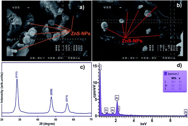
FE-SEM of ZnS-NPs-AC (Fig. 1a and b) reveals its amorphous morphology and/or the spherical shape with sizes in the range of 50–100 nm.The XRD pattern of the ZnO nanospheres (Fig. 1c) consists of (111), (220) and (311) peaks corresponding to the zinc blende structure (cubic, b-ZnS; JCPDS no. 05-0566). The peak broadening in the XRD pattern clearly indicates the presence of nanocrystals of ZnS with very small size, while the average size based on the Debye–Scherrer formula (D = 0.89λ/β![[thin space (1/6-em)]](https://www.rsc.org/images/entities/char_2009.gif) cosθ) using the (111) diffraction peak is around 40 nm.
cosθ) using the (111) diffraction peak is around 40 nm.
Energy dispersive X-ray spectroscopy (EDS) of the ZnS-NPs-AC (Fig. 1d) based on the localized elemental information shows the presence of C, Zn and S as the dominant elements throughout the surface of the adsorbent, with weight percentages of 95.30, 2.60 and 2.10%, respectively.
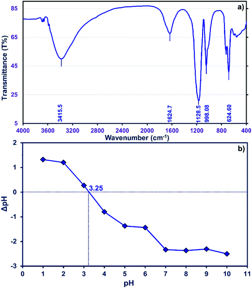
The FTIR spectrum of the ZnS nanoparticles (Fig. 2a) is composed of peaks around 1128.5, 998.08, and 624.60 cm−1 showing good agreement with previously reported results.41,42 The observed peak at 1624.7 cm−1 is assigned to the C![[double bond, length as m-dash]](https://www.rsc.org/images/entities/char_e001.gif) O stretching mode, while broad absorption peaks in the 3100–3600 cm−1 interval correspond to O–H stretching modes arising from the absorption of water on the surface of the nanoparticles via –COOH groups or even the AC functional groups.
O stretching mode, while broad absorption peaks in the 3100–3600 cm−1 interval correspond to O–H stretching modes arising from the absorption of water on the surface of the nanoparticles via –COOH groups or even the AC functional groups.
The neutral charge of the adsorbent surface at pHZPC becomes negative at pH values higher and positive at pH values lower than this value, respectively.43 Data of ΔpH (pHfinal − pHinitial) vs. pH were plotted (Fig. 2b) and reveal that pHzpc is 3.25 for ZnS-NPs-AC. Therefore, at pH values greater than 3.25 the removal should be higher due to increased electrostatic interactions. Generally, the net positive charge of adsorbate decreases at higher pH and is associated with a decrease in the repulsion between the adsorbent surface and the cationic MB dye.
3.2. CCD model and statistical analysis
RSM is an efficient technique for optimization and was applied to analyze the effect of the important parameters and their interactions on the adsorption process under different conditions using CCD.15The factors affecting MB removal efficiency should be more keenly monitored so that better systems can be developed to remove dyes from waste waters on a pilot scale. Hence, in this study, the CCD was applied to optimize the adsorption of MB dye from dye solution by varying the parameters pH, adsorbent mass, MB concentration and contact time in the preliminary steps, while the numerical values of various runs and respective experimental responses are detailed in Table 1.
The analysis of CCD results led to the following second-order polynomial equation:
YR% MB = −8.3 + 18.6X1 + 4512.7X2 − 0.2X3 + 2.9X4 − 171.5X1X2 − 0.02X1X3 − 0.81X1X4 + 6.71X2X3 + 118.1X2X4 + 0.13X3X4 − 0.93X12 − 101![[thin space (1/6-em)]](https://www.rsc.org/images/entities/char_2009.gif) 476.22X22 − 0.01X32 − 0.24X42 476.22X22 − 0.01X32 − 0.24X42
| (8) |
ANOVA based on F- and P-tests gives information about the type of contribution of each term to the response and quality of the regression equation (Table 2).
| Source of variation | Sum of square | Degree of freedom | Mean square | F-value | P-value | Status | Regression coefficients | |
|---|---|---|---|---|---|---|---|---|
| Factor | Coefficient estimate | |||||||
| Model | 927.0695 | 14 | 66.2192 | 448.0346 | <0.0001 | Significant | Intercept | −8.325 |
| X1-pH | 51.7470 | 1 | 51.7470 | 350.1165 | <0.0001 | X1 | +18.560 | |
| X2-adsorbent mass | 452.9279 | 1 | 452.9279 | 3064.4772 | <0.0001 | X2 | +4513.0 | |
| X3-MB concentration | 53.4882 | 1 | 53.4882 | 361.8974 | <0.0001 | X3 | −0.172 | |
| X4-sonication time | 30.4223 | 1 | 30.4223 | 205.8349 | <0.0001 | X4 | +2.901 | |
| X1X2 | 26.4736 | 1 | 26.4736 | 179.1184 | <0.0001 | X1X2 | −171.5 | |
| X1X3 | 1.0267 | 1 | 1.0267 | 6.9464 | 0.01872 | X1X3 | −0.021 | |
| X1X4 | 23.4425 | 1 | 23.4425 | 158.6105 | <0.0001 | X1X4 | −0.807 | |
| X2X3 | 1.1519 | 1 | 1.1519 | 7.7934 | 0.01369 | X2X3 | +6.708 | |
| X2X4 | 5.5779 | 1 | 5.5779 | 37.7394 | <0.0001 | X2X4 | +118.10 | |
| X3X4 | 17.2536 | 1 | 17.2536 | 116.7369 | <0.0001 | X3X4 | +0.130 | |
| X12 | 119.8745 | 1 | 119.8745 | 811.0625 | <0.0001 | X12 | −0.929 | |
| X22 | 176.5272 | 1 | 176.5272 | 1194.3705 | <0.0001 | X22 | −101![[thin space (1/6-em)]](https://www.rsc.org/images/entities/char_2009.gif) 500.0 500.0 |
|
| X32 | 6.5670 | 1 | 6.5670 | 44.4316 | <0.0001 | X32 | −0.008 | |
| X42 | 1.5284 | 1 | 1.5284 | 10.3410 | 0.005775 | X42 | −0.236 | |
| Residual | 2.2170 | 15 | 0.1478 | |||||
| Lack of fit | 0.7745 | 10 | 0.0775 | 0.2685 | 0.9635 | Not significant | ||
| Pure error | 1.4424 | 5 | 0.2885 | |||||
| Cor total | 929.2865 | 29 | ||||||
| Quadratic summary statistics | R2 | Adj-R2 | Pred-R2 | Std dev. | CV% | PRESS | Adequate precision |
|---|---|---|---|---|---|---|---|
| Response (R% MB) | 0.9976 | 0.9954 | 0.9930 | 0.3844 | 0.4135 | 6.539 | 75.92 |
The statistical significance of the model is assigned according to the F-value. The “Model F-value” of 448.035 is a good indication of the high efficiency and applicability of the present model and denotes that there is only 0.01% chance of obtaining this value due to noise. A very low probability value (P-value < 0.0001) implies that the model is strongly significant at a 95% confidence interval (i.e., P-values less than 0.05 indicate significance). The non-significant lack-of-fit is favorable and specifies the high predictability of the model. The “Lack of Fit F-value” (0.2685) strongly indicates its low contribution compared to pure error. In Table 2, the P-values < 0.050 are significant.
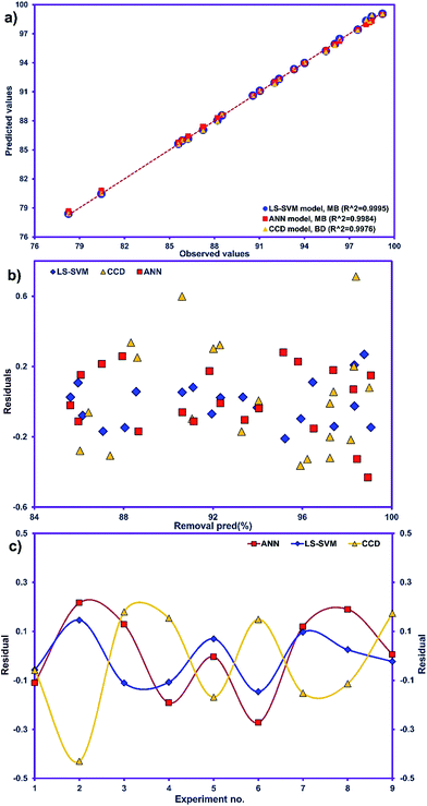
The R2 value of 0.9976 indicates that 99.76% of the variability can be explained in random fashion changes in the variable. The R2-predicted value of 0.9930 is in reasonable agreement with the R2-adjusted value of 0.9954. Fig. 3a indicates that the predicted values of MB adsorption efficiency obtained from the model and the actual experimental data are in good agreement which is evidence for the validity of the regression model. Fig. 3b shows the residual plot versus predicted data and the random pattern of residuals exhibits the model's adequacy.
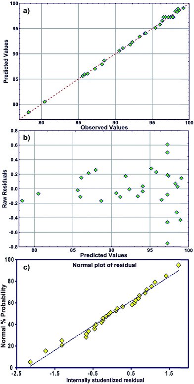 | ||
| Fig. 3 (a) Plot of the measured and model-predicted values of the response variable, (b) residuals versus predicted removal percentage (R%) and (c) the normal probability plot of the residuals. | ||
An adequate precision (signal-to-noise ratio) value higher than 4 supports the desirability of the model; a value of 75.92 was found in the present study. Hence this model can navigate the design space.44 The degree of precision and reliability given by the coefficient of variation (CV) (0.4135%) shows the higher precision and reliability of experimental data.45
The normal distribution of data was traced by plotting the residuals and deviations of the observed data values from the predicted values (Fig. 3c). A visual examination of the data shows that the data points fall approximately along a straight line for MB adsorption and also suggests the fair adequacy of the constructed equation for predicting the adsorption and estimating individual interactions between the response and process parameters.
3.3. Model graphs for the effect of variables
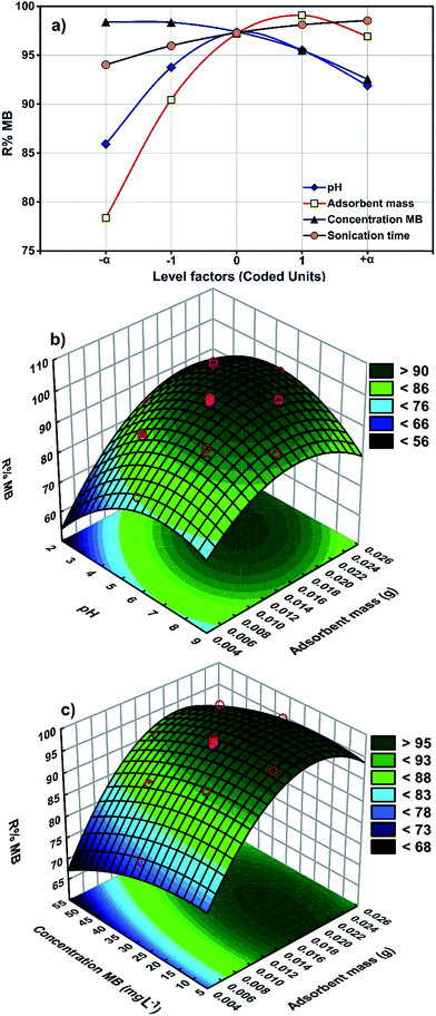
The results from a plot of perturbation response (R% MB) against the factors (Fig. 4a) show evidence for the importance of pH (X1), adsorbent mass (X2), MB concentration (X3) and sonication time (X4) in the MB removal process. Fig. 4 shows the MB removal percentage in terms of raising each variable in turn while all other factors are held in the middle of the design space (the coded zero level). The influence of the adsorbent mass on the removal percentage became more pronounced when moving from the middle towards the higher levels. The reciprocal slope of the perturbation curve for factor X2 (MB concentration) is related to a decrease in MB removal when increasing the MB concentration up to 40 mg L−1. The reciprocal slope of the perturbation curve for X1 and X4 (pH and sonication time) confirmed that maximum MB removal is seen at pH 7.0 and 5 min.The main effects of each parameter on the MB removal efficiency (Fig. 4) show that both pH and adsorbent mass have a positive correlation with the removal percentage (Fig. 4b) that is attributed to the increase in availability of binding sites at a higher initial solution pH and the enhancement of the accessibility of dye for binding sites of adsorbent.43 The problem with high adsorbent mass however is that it may cause interference between binding sites or there may be insufficient dye ions in the solution with respect to the available binding sites. It is likely that protons will then combine with dye ions and thereby decrease the interaction of dye ions with the ZnS-NP-AC components.
The pHzpc of ZnS-NP-AC was equal to 3.25 (Fig. 2b) and therefore, basic solution favors MB adsorption onto the ZnS-NP-AC. This is favorable for the studied adsorption system for real waste water decolorization from the textile industry (alkaline) because it avoids additional costs for pH control.
The combined effects of adsorbent mass and MB concentration (Fig. 4c) reveal the reverse impact of MB concentration and adsorbent mass on MB uptake. At lower adsorbent mass, an increase in MB concentration led to saturation of the binding sites and finally a decline in uptake. A higher adsorbent mass enhanced the uptake which may be related to the availability of relatively more active binding sites.
3.4. Analysis of AAN
In this research, ANN models have been used to evaluate the effect of four input variables, namely pH, adsorbent mass, MB concentration and sonication time, on the removal percentage of MB as the output. A feed-forward topology of the ANN model, famous as a multilayer perceptron (MLP), has been used with a BP algorithm to build the predictive models.The optimization of the network is a very important step in network training that is based on the optimization of a number of neurons in the hidden layer. For this purpose, different numbers of neurons (2–15 neurons corresponding to the hidden layer) were tested and it was found that a hidden layer with 8 neuron was the best case and permitted achievement of good operation parameters with a minimum value of MSE and a maximum value of R2. As a result, in this study a three layered feed-forward BP ANN (4![[thin space (1/6-em)]](https://www.rsc.org/images/entities/char_2009.gif) :
:![[thin space (1/6-em)]](https://www.rsc.org/images/entities/char_2009.gif) 8
8![[thin space (1/6-em)]](https://www.rsc.org/images/entities/char_2009.gif) :
:![[thin space (1/6-em)]](https://www.rsc.org/images/entities/char_2009.gif) 1) was used for modeling of the adsorption process. Fig. 5a displays the goodness of fit between the forecast values for the removal of data using the ANN model against the actual values for the CCD matrix.
1) was used for modeling of the adsorption process. Fig. 5a displays the goodness of fit between the forecast values for the removal of data using the ANN model against the actual values for the CCD matrix.
3.5. Analysis of LS-SVM
The constructed LS-SVM model with the RBF kernel function was applied to the selected data set to predict MB adsorption using the set of four variables as estimators. A two-step grid search method with a tenfold cross-validation was used to derive the LS-SVM model parameters. The optimal values for the LS-SVM model parameters, C (cost constant), ε (the radius of the insensitive tube) and kernel-dependent parameter (γ) were found to be 672.34, 0.002, and 1.327, respectively, and the number of SVs was 185; the statistical parameter values are summarized in Table 3. It may be noted that the model-predicted values of the dependent variable have a high correlation with the experimental values in all three sets (R2 was 0.9997 in training and 0.9996 for the validation data). Values of other criteria parameters suggest a good fit of the LS-SVM model to the datasets and the adequacy of the selected model for predicting the adsorptive removal of MB.| Models | Statistical parameters | |||
|---|---|---|---|---|
| R2 | RMSE | AAD% | MAE | |
| LS-SVM | 0.9995 | 0.000229747 | 0.000600812 | 0.101417559 |
| ANN | 0.9984 | 0.000989432 | −0.033166815 | 0.145769511 |
| RSM (CCD) | 0.9976 | 0.001233283 | −0.003189788 | 0.157790909 |
3.6. Comparison of RSM with ANN and LS-SVM
The capabilities of the proposed LS-SVM, ANN and RSM techniques for the prediction and modeling of the MB adsorption system were evaluated by means of comparing the responses computed from each method to the observed data. For this purpose, the techniques were used to predict the responses belonging to 30 experimental points (the CCD matrix). The performances of the constructed LS-SVM, ANN and RSM models were also statistically measured by R2 values, RMSE, mean absolute error (MAE) and absolute average deviation (AAD) as follows:
 | (9) |
 | (10) |
 | (11) |
 | (12) |
R2 measures the percentage of total variation in the response variable that is explained by least-squares regression. R2 must be closed to 1.0, whereas AAD, which is a direct method for describing deviations between predicted and experimental data, must be as small as possible.
Table 3 presents the statistical comparison (i.e. R2, RMSE, AAD and MAE) of RSM, LS-SVN and ANN models. Generally, all three (RSM, LS-SVM and ANN) models provided good quality predictions in this study; they can be considered to perform well in data fitting and offered stable responses. However, the LS-SVM showed a clear superiority over ANN and RSM. On the other hand, values of the model prediction errors suggest that the RSM prediction performance was relatively poor as compared with the other models applied here. This finding is similar to the usual notion that ANN and SVM regression give better performances than RSM.46 Residuals versus predicted value plots can be more informative regarding model fitting to a data set. If the residuals appear to behave randomly it suggests that the model fits the data well. On the other hand, if a non-random distribution is evident in the residuals, the model does not fit the data adequately. The model-predicted values of the response variable and the residuals corresponding to the experimental data set are plotted in Fig. 5b. The observed relationship between residuals and model-predicted values of removal (R%) yielded by all the three models used here show random distribution and almost complete independence.
The goodness-of-fit between the experimental and the predicted responses given by the LS-SVM, ANN and RSM models are shown in Fig. 5a. The residuals (the differences between predicted and actual values) for both approaches are shown in Fig. 5c which shows the distribution of residuals of the three approaches as a criterion for their compression. The fluctuations of the residuals are relatively small and regular for SVM compared to ANN and RSM. The RSM model shows greater deviation than the LS-SVM and ANN models.
However, there is no vagueness in the RSM model compared with the other approaches, because the RSM model presents all of the relationships between linear, interaction and quadratic effects. Furthermore, the RSM model plays an important role in decreasing the number of experiments, cost and time. In addition, the RSM model optimized the conditions and developed a full quadratic model at optimum conditions.
3.7. Analysis of CCD combined with DF and GA
After performing the experimental design, the response surface and contour plot were drawn using STATISTICA software to guide the determination of optimum values. The optimum values were found to be 7.0, 20 mg L−1, 0.015 g and 3 min for the variables pH, initial MB concentration, adsorbent mass and sonication time, respectively and led to the achievement of a 98.19% removal percentage which was strongly confirmed by five replicates at these conditions that led to a 98.02% ± MB removal percentage.GA using Matlab R2015a was applied to optimize the input fitness functions formulated in eqn (9) of the CCD for all parameters. According to Table 1, high and low values of each parameter were used to achieve the maximum MB simultaneous removal following the optimization of conditions by GA.
GA optimized values were found to be 6.99, 0.015 g, 20.001 g and 2.994 min for pH, adsorbent mass, MB concentration, and sonication time, respectively. This result was cross-validated by carrying out the batch study at the aforementioned GA-specified optimum conditions. Fig. 6 represents the best fitness plot achieved during the iterations of GA over 50 generations and describes the gradual convergence of results towards the optimal solution.
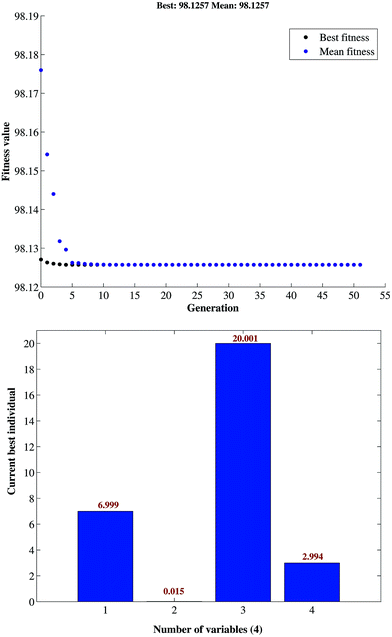 | ||
| Fig. 6 Plot of fitness value vs. generation for the variables in GA optimization of the removal of MB. | ||
The optimum conditions for the ultrasound-assisted removal of MB predicted by DF and GA are further compared with experimental results for the same set of parameters (Table 4). This comparison shows a good agreement between the experimental and the predicted data.
| Factors | Models | |
|---|---|---|
| CCD-DF | CCD-GA | |
| pH | 7.000 | 6.999 |
| Adsorbent mass (mg) | 0.015 | 0.015 |
| MB concentration (mg L−1) | 20.000 | 20.001 |
| Sonication time (min) | 3.000 | 2.994 |
| R%MB | 98.02 | 98.125 |
3.8. Kinetic studies
The adsorption kinetics of MB onto ZnS-NP-AC were investigated using four kinetic models, namely, the pseudo-first-order,47 pseudo-second-order,48 intraparticle diffusion49 and Elovich50 models.The linear plots for pseudo-first-order (Fig. 7a) and pseudo-second-order (Fig. 7b) kinetic models were used to find the values of their respective parameters. The R2 values and the various kinetic parameters obtained from the applied kinetic models are shown in Table 5. The values of R2 for the pseudo-first-order (≤0.9770), intraparticle diffusion (≤0.9737) and Elovich (≤0.9894) kinetic models were low. On the other hand, the values of R2 for the pseudo-second-order kinetic model were ≥0.9983 in most situations and the very reasonable closeness of experimental and predicted qe values confirmed the high efficiency of this model for representation of the experimental data (Table 5).
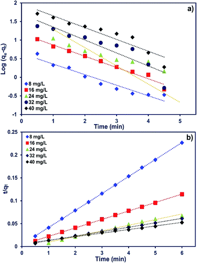 | ||
| Fig. 7 (a) Pseudo-first-order and (b) second-order kinetic plots for MB adsorption on ZnS-NP-AC (dye concentration: 8–40 mg L−1, adsorbent mass: 0.015 g and pH: 7.0). | ||
3.9. Adsorption isotherms
The equilibrium adsorption isotherms are fundamental in describing the interactive behavior between adsorbates and adsorbent and are essential for giving an idea of the adsorption capacity of the adsorbent. In the present study, four adsorption isotherm models, the Langmuir,51 Freundlich,52 Temkin53 and Dubinin-Radushkevich (D-R)54 equations, were used to describe the adsorption equilibrium. The Langmuir isotherm is the most popular isotherm model and it is mainly applied to describe monolayer adsorption processes. The Freundlich model is a semi-empirical equation describing heterogeneous surface adsorption and multilayer adsorption under various non-ideal conditions. The Temkin isotherm describes a state in which the heat of adsorption falls linearly with increasing adsorption capacity. D-R is generally applied to express an adsorption mechanism with a Gaussian energy distribution onto a heterogeneous surface.All adsorption isotherm parameters and R2 values corresponding to each model are listed in Table 6 based on the respective plots for each model: Ce/qe vs. Ce, ln![[thin space (1/6-em)]](https://www.rsc.org/images/entities/char_2009.gif) qe vs. ln
qe vs. ln![[thin space (1/6-em)]](https://www.rsc.org/images/entities/char_2009.gif) Ce, qe vs. ln
Ce, qe vs. ln![[thin space (1/6-em)]](https://www.rsc.org/images/entities/char_2009.gif) Ce and ln
Ce and ln![[thin space (1/6-em)]](https://www.rsc.org/images/entities/char_2009.gif) qe vs. ε2 straight line plots for the Langmuir, Freundlich, Temkin and D-R models, respectively (Fig. 8a–d).
qe vs. ε2 straight line plots for the Langmuir, Freundlich, Temkin and D-R models, respectively (Fig. 8a–d).
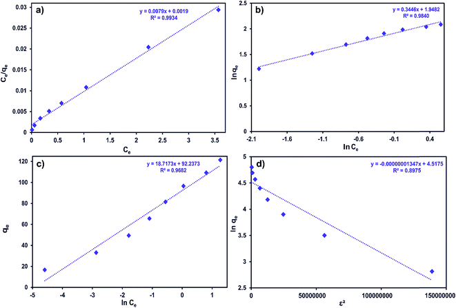 | ||
| Fig. 8 (a) Langmuir, (b) Freundlich, (c) Temkin and (d) D-R adsorption isotherms for the adsorption of MB onto ZnS-NP-AC (adsorbent mass: 0.015 g, sonication time: 3 min and pH: 7.0). | ||
As can be seen from Table 6, the correlation coefficients and error analysis support the high efficiency of the Langmuir equation (R2 ≥ 0.9934) for representing the equilibrium experimental data with a maximum adsorption capacity (Qm) of 234.90 mg g−1. The RL values of 0.0022–0.1316 (Table 6) support this high ability and favorability. The less than unity values of 1/n point towards a favorable adsorption process. The R2 values (0.7083–0.9849) for the Freundlich, Temkin and D-R isotherms indicate that these isotherms are not appropriate to describe the experimental data for MB adsorption.
The E value obtained using the D-R constant gives information about adsorption mechanism, physical or chemical. If it lies between 8 and 16 kJ mol−1, the adsorption process takes place chemically, while if E < 8 kJ mol−1, the adsorption process proceeds physically. The E values obtained for all adsorbent masses studied in this research were lower than 8 kJ mol−1, which shows that the adsorption of MB onto ZnS-NP-AC occurs by physisorption.
3.10. Performance comparison with other adsorbents
Table 7 compares the sorption capacity (mg g−1), pH and contact time (min) of different nanoparticle adsorbents used for the removal of MB. The value of Qm in this study using an environmentally friendly and low cost adsorbent is significantly higher than those obtained in most of the previous work. As seen in Table 7, the present method is highly recommended due to its higher adsorption capacity over a short time and usage of a small amount of adsorbent, and is favorable for waste water treatment. The present method is preferred and superior to the literature methods in terms of its satisfactory removal performance for dyes as compared to other reported adsorbents.| Adsorbent | pH | Sorption capacity (mg g−1) | Contact time (min) | Ref. |
|---|---|---|---|---|
| MWCNTs filled with Fe2O3 particles | 6.0 | 42.90 | 60 | 55 |
ZnS![[thin space (1/6-em)]](https://www.rsc.org/images/entities/char_2009.gif) : :![[thin space (1/6-em)]](https://www.rsc.org/images/entities/char_2009.gif) Cu nanoparticles loaded on activated carbon Cu nanoparticles loaded on activated carbon |
7.0 | 106.95 | 2.2 | 50 |
| Ag nanoparticles loaded on activated carbon | 2.5 | 71.43 | 15 | 14 |
| Au nanoparticles loaded on activated carbon | 7.0 | 185.00 | 1.6 | 56 |
| Mn–Fe3O4 nanoparticles loaded on activated carbon | 5.0 | 229.40 | 3.0 | 44 |
| Fe3O4 nanoparticles | 6.0 | 91.90 | 2.0 | 57 |
| Oxidized multiwalled carbon nanotubes (MWCNT) | 6.0 | 102.3 | 2.6 | 58 |
| Graphene nanosheet/magnetite (Fe3O4) composite | 6.0 | 43.83 | 20 | 9 |
| NiS nanoparticles loaded on activated carbon | 8.1 | 52.00 | 5.46 | 13 |
| CuO nanoparticles loaded on activated carbon | 7.0 | 10.55 | 15 | 59 |
| MnO2 nanoparticles loaded on activated carbon | 7.0 | 234.20 | 4.0 | 43 |
| ZnO nanorods loaded on activated carbon | 7.0 | 238.09 | 20 | 8 |
| γ-Fe2O3-NPs-AC | 7.0 | 195.55 | 4.0 | 4 |
| Ru nanoparticles loaded on activated carbon | 7.0 | 185.185 | 27 | 60 |
| ZnS nanoparticles loaded on activated carbon | 7.0 | 243.90 | 3.0 | This study |
3.11. Recycling
Regeneration of the adsorbents is important for economic and resource reasons. To assess the adsorption efficiency of the recycled ZnS-NP-AC over nine consecutive cycles, experimental tests were carried out using 50 mL of 20 mg L−1 MB solutions, 0.015 g adsorbent and 3 min sonication. Subsequently, the mixture was centrifuged for 3 min at 3000 rpm and the MB adsorption percentage was determined to be 98.20%. The adsorbed MB was efficiently eluted by 10 mL methanol (Fig. 9) and less than 10% in MB removal was seen, while at higher times MB molecules strongly attached to the ZnS-NP-AC via chemical adsorption.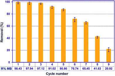 | ||
| Fig. 9 Effect of the number of regeneration cycles on the adsorption of MB onto ZnS-NP-AC (MB concentration: 20 mg L−1, adsorbent mass: 0.015 g, sonication time: 3 min and pH: 7.0). | ||
4. Conclusions
In this study, the main objective was the development and construction of a novel model that could make a reliable prediction of MB adsorption onto ZnS-NPs-AC on the basis of batch adsorption experiments performed with four different process variables (pH, adsorbent mass, MB concentration, and sonication time). LS-SVM, ANN and RSM models were constructed for predicting the removal of MB. Generalization and predictive performances of the different models were evaluated using the statistical criteria of RMSE, R2, MAE and AAD and analysis of the residuals. All three models predicted the adsorption of MB by ZnS-NPs-AC from aqueous solutions satisfactorily. Based on the findings, the present work indicates that the LS-SVM is much more accurate in modeling the removal of MB dye than the ANN or RSM models. The experimental data from CCD were excellently fitted to the quadratic model, and the relationship between the response and the variables was described by a second-order polynomial equation (regression model). The dosage of ZnS-NPs-AC was the most significant factor for dye removal, followed by pH and sonication time, and the least significant factor was dye concentration. CCD combined with DF and GA methods showed the maximum uptake efficiency for different combinations of pH and MB concentration. The predicted maximum MB adsorption with the corresponding optimal parameters for the adsorption process using DF and GA were as follows: pH 7.00 and 6.99, adsorbent mass 0.015 and 0.015, MB concentration 20.000 and 20.001 mg L−1, and sonication time 3.000 and 2.994 min, respectively. The MB removal process obeys a pseudo-second-order kinetic expression. Adsorption of MB onto the adsorbent follows the Langmuir isotherm. A regeneration study of the material was also carried out and it was found that the ZnS-NP-AC could be regenerated using methanol solution and reused. This report can be used as a stimulus for motivating and inspiring other researchers to develop advanced and optimized systems based on adsorption for the nontoxic and effective treatment of waste water.Acknowledgements
The authors express their appreciation to the Graduate School and Research Council of the Yasouj University for their financial support.References
- L. Cui, X. Guo, Q. Wei, Y. Wang, L. Gao, L. Yan, T. Yan and B. Du, J. Colloid Interface Sci., 2015, 439, 112–120 CrossRef CAS PubMed.
- V. K. Gupta, R. Jain, T. Saleh, A. Nayak, S. Malathi and S. Agarwal, Sep. Sci. Technol., 2011, 46, 839–846 CrossRef CAS.
- S. Dutta, A. Bhattacharyya, A. Ganguly, S. Gupta and S. Basu, Desalination, 2011, 275, 26–36 CrossRef CAS.
- A. Asfaram, M. Ghaedi, S. Hajati and A. Goudarzi, Ultrason. Sonochem., 2016, 32, 418–431 CrossRef CAS.
- M. T. Uddin, M. A. Islam, S. Mahmud and M. Rukanuzzaman, J. Hazard. Mater., 2009, 164, 53–60 CrossRef CAS PubMed.
- A. Asfaram, M. Ghaedi, S. Hajati, A. Goudarzi and A. A. Bazrafshan, Spectrochim. Acta, Part A, 2015, 145, 203–212 CrossRef CAS PubMed.
- Y. C. Sharma, J. Chem. Eng. Data, 2009, 55, 435–439 CrossRef.
- M. Ghaedi, A. G. Nasab, S. Khodadoust, R. Sahraei and A. Daneshfar, J. Ind. Eng. Chem., 2015, 21, 986–993 CrossRef CAS.
- L. Ai, C. Zhang and Z. Chen, J. Hazard. Mater., 2011, 192, 1515–1524 CrossRef CAS PubMed.
- F. N. Azad, M. Ghaedi, A. Asfaram, A. Jamshidi, G. Hassani, A. Goudarzi, M. H. A. Azqhandi and A. Ghaedi, RSC Adv., 2016, 6, 19768–19779 RSC.
- F. Nasiri Azad, M. Ghaedi, K. Dashtian, M. Montazerozohori, S. Hajati and E. Alipanahpour, RSC Adv., 2015, 5, 61060–61069 RSC.
- S. Hajati, M. Ghaedi and S. Yaghoubi, J. Ind. Eng. Chem., 2015, 21, 760–767 CrossRef CAS.
- M. Ghaedi, M. Pakniat, Z. Mahmoudi, S. Hajati, R. Sahraei and A. Daneshfar, Spectrochim. Acta, Part A, 2014, 123, 402–409 CrossRef CAS PubMed.
- M. Ghaedi, S. Heidarpour, S. Nasiri Kokhdan, R. Sahraie, A. Daneshfar and B. Brazesh, Powder Technol., 2012, 228, 18–25 CrossRef CAS.
- A. Ahmad, S. H. Mohd-Setapar, C. S. Chuong, A. Khatoon, W. A. Wani, R. Kumar and M. Rafatullah, RSC Adv., 2015, 5, 30801–30818 RSC.
- S. Agarwal, I. Tyagi, V. K. Gupta, A. R. Bagheri, M. Ghaedi, A. Asfaram, S. Hajati and A. A. Bazrafshan, J. Environ. Chem. Eng., 2016, 4, 1769–1779 CrossRef CAS.
- M. K. Sahu, U. K. Sahu and R. K. Patel, RSC Adv., 2015, 5, 42294–42304 RSC.
- A. Asfaram, M. Ghaedi and G. R. Ghezelbash, RSC Adv., 2016, 6, 23599–23610 RSC.
- P. Cakir, S. Inan and Y. Altas, J. Hazard. Mater., 2014, 271, 108–119 CrossRef CAS PubMed.
- G. B. Sahoo, C. Ray, E. Mehnert and D. A. Keefer, Sci. Total Environ., 2006, 367, 234–251 CrossRef CAS PubMed.
- T. Rajaee, S. A. Mirbagheri, M. Zounemat-Kermani and V. Nourani, Sci. Total Environ., 2009, 407, 4916–4927 CrossRef CAS PubMed.
- K. Yetilmezsoy and S. Demirel, J. Hazard. Mater., 2008, 153, 1288–1300 CrossRef CAS PubMed.
- N. G. Turan, B. Mesci and O. Ozgonenel, Chem. Eng. J., 2011, 171, 1091–1097 CrossRef CAS.
- R. L. Haupt and S. E. Haupt, Practical genetic algorithms, John Wiley & Sons, 2004 Search PubMed.
- S. Kim, K.-S. Sohn and M. Pyo, ACS Comb. Sci., 2011, 13, 101–106 CrossRef CAS PubMed.
- M. Roosta, M. Ghaedi and A. Asfaram, RSC Adv., 2015, 5, 57021–57029 RSC.
- A. Asfaram, M. Ghaedi, S. Agarwal, I. Tyagi and V. Kumar Gupta, RSC Adv., 2015, 5, 18438–18450 RSC.
- M. Ghaedi, H. Z. Khafri, A. Asfaram and A. Goudarzi, Spectrochim. Acta, Part A, 2016, 152, 233–240 CrossRef CAS PubMed.
- M. Ghaedi, E. Alam barakat, A. Asfaram, B. Mirtamizdoust, A. A. Bazrafshan and S. Hajati, RSC Adv., 2015, 5, 42376–42387 RSC.
- A. R. Bagheri, M. Ghaedi, S. Hajati, A. M. Ghaedi, A. Goudarzi and A. Asfaram, RSC Adv., 2015, 5, 59335–59343 RSC.
- M. Turabık and B. Gozmen, Clean: Soil, Air, Water, 2013, 41, 1080–1092 CrossRef.
- V. Vapnik, The nature of statistical learning theory, Springer Science & Business Media, 2013 Search PubMed.
- J. A. Suykens, Eur. J. Contr., 2001, 7, 311–327 CrossRef.
- K. P. Singh, S. Gupta, P. Ojha and P. Rai, Environ. Sci. Pollut. Res., 2013, 20, 2271–2287 CrossRef CAS PubMed.
- N. Cristianini and J. Shawe-Taylor, An introduction to support vector machines and other kernel-based learning methods, Cambridge university press, 2000 Search PubMed.
- M. Ghaedi, M. Reza Rahimi, A. Ghaedi, I. Tyagi, S. Agarwal and V. K. Gupta, J. Colloid Interface Sci., 2016, 461, 425–434 CrossRef CAS PubMed.
- E. A. Dil, M. Ghaedi, A. M. Ghaedi, A. Asfaram, A. Goudarzi, S. Hajati, M. Soylak, S. Agarwal and V. K. Gupta, J. Ind. Eng. Chem., 2016, 34, 186–197 CrossRef CAS.
- A. Bouchachia, Adaptive and Intelligent Systems: Third International Conference, ICAIS 2014, Bournemouth, UK, September 8-9, 2014, Proceedings, Springer, 2014 Search PubMed.
- A. Khataee and M. Kasiri, J. Mol. Catal. A: Chem., 2010, 331, 86–100 CrossRef CAS.
- F. Nasiri Azad, M. Ghaedi, K. Dashtian, M. Montazerozohori, S. Hajati and E. Alipanahpour, RSC Adv., 2015, 5, 61060–61069 RSC.
- M. Kuppayee, G. K. Vanathi Nachiyar and V. Ramasamy, Appl. Surf. Sci., 2011, 257, 6779–6786 CrossRef CAS.
- I. Parvaneh, S. Samira and N. Mohsen, Chin. Phys. B, 2015, 24, 46–50 Search PubMed.
- A. Asfaram, M. Ghaedi, S. Hajati and A. Goudarzi, RSC Adv., 2015, 5, 72300–72320 RSC.
- A. Asfaram, M. Ghaedi, A. Goudarzi and M. Rajabi, Dalton Trans., 2015, 44, 14707–14723 RSC.
- M. Ghaedi, Z. Rozkhoosh, A. Asfaram, B. Mirtamizdoust, Z. Mahmoudi and A. A. Bazrafshan, Spectrochim. Acta, Part A, 2015, 138, 176–186 CrossRef CAS PubMed.
- M. Jamshidi, M. Ghaedi, K. Dashtian, A. M. Ghaedi, S. Hajati, A. Goudarzi and E. Alipanahpour, Spectrochim. Acta, Part A, 2016, 153, 257–267 CrossRef CAS PubMed.
- Y. Tang, T. Hu, Y. Zeng, Q. Zhou and Y. Peng, RSC Adv., 2015, 5, 3757–3766 RSC.
- T. G. Yan and L. J. Wang, Water Sci. Technol., 2014, 69, 612–621 CrossRef CAS PubMed.
- Z. Ioannou and J. Simitzis, Water Sci. Technol., 2013, 67, 1688–1694 CrossRef CAS PubMed.
- A. Asfaram, M. Ghaedi, S. Hajati, M. Rezaeinejad, A. Goudarzi and M. K. Purkait, J. Taiwan Inst. Chem. Eng., 2015, 53, 80–91 CrossRef CAS.
- J. Fu, Z. Chen, M. Wang, S. Liu, J. Zhang, J. Zhang, R. Han and Q. Xu, Chem. Eng. J., 2015, 259, 53–61 CrossRef CAS.
- J. J. Gao, Y. B. Qin, T. Zhou, D. D. Cao, P. Xu, D. Hochstetter and Y. F. Wang, J. Zhejiang Univ., Sci., B, 2013, 14, 650–658 CrossRef CAS PubMed.
- L. Ai, C. Zhang, F. Liao, Y. Wang, M. Li, L. Meng and J. Jiang, J. Hazard. Mater., 2011, 198, 282–290 CrossRef CAS PubMed.
- F. N. Azad, M. Ghaedi, K. Dashtian, S. Hajati and V. Pezeshkpour, Ultrason. Sonochem., 2016, 31, 383–393 CrossRef CAS PubMed.
- S. Qu, F. Huang, S. Yu, G. Chen and J. Kong, J. Hazard. Mater., 2008, 160, 643–647 CrossRef CAS PubMed.
- M. Roosta, M. Ghaedi, A. Daneshfar, R. Sahraei and A. Asghari, Ultrason. Sonochem., 2014, 21, 242–252 CrossRef CAS PubMed.
- M. Ghaedi, S. Hajjati, Z. Mahmudi, I. Tyagi, S. Agarwal, A. Maity and V. Gupta, Chem. Eng. J., 2015, 268, 28–37 CrossRef CAS.
- M. Ghaedi, S. Hajati, M. Zare, M. Zare and S. Y. Shajaripour Jaberi, RSC Adv., 2015, 5, 38939–38947 RSC.
- M. Ghaedi, A. Ghaedi, M. Hossainpour, A. Ansari, M. Habibi and A. Asghari, J. Ind. Eng. Chem., 2014, 20, 1641–1649 CrossRef CAS.
- H. Mazaheri, M. Ghaedi, S. Hajati, K. Dashtian and M. K. Purkait, RSC Adv., 2015, 5, 83427–83435 RSC.
Footnote |
| † Electronic supplementary information (ESI) available. See DOI: 10.1039/c6ra01874b |
| This journal is © The Royal Society of Chemistry 2016 |

