
Removal of cationic and anionic dyes from aqueous solution with magnetite/pectin and magnetite/silica/pectin hybrid nanocomposites: kinetic, isotherm and mechanism analysis†
Olivia A. Attallaha,
Medhat A. Al-Ghobashybc,
Marianne Nebsen*ab and
Maissa Y. Salemb
aPharmaceutical Chemistry Department, Faculty of Pharmacy, Heliopolis University, Egypt
bAnalytical Chemistry Department, Faculty of Pharmacy, Cairo University, Egypt. E-mail: marianne.morcos@pharma.cu.edu.eg
cBioanalysis Research Group, Faculty of Pharmacy, Cairo University, Egypt
First published on 28th January 2016
Abstract
Novel adsorbents, magnetite nanoparticles modified with pectin shell and silica/pectin double shell, were fabricated and tested for single dye and dye mixture adsorption from water samples. Cationic dyes methylene blue (MB) and crystal violet (CV) and anionic dyes methyl orange (MO) and Eriochrome black T (EBT) were employed to assess dye removal efficiency. The influence of pH, amount of adsorbent, initial dye concentration and contact time was investigated. Results indicated that the optimum pH for removing cationic dyes was 8.0 and 2.0 for anionic dyes. The kinetic studies showed rapid sorption dynamics following a second-order kinetic model. Dye adsorption equilibrium data were fitted well to the Sips isotherm for cationic and anionic dyes. The maximum monolayer capacity, (qmax) for MB, CV, EBT and MO was calculated from Sips as 197.18, 180.29, 65.35 and 26.75 mg g−1 respectively for magnetite/silica/pectin NPs and 168.72, 140.49, 72.35 and 27.22 mg g−1 respectively for magnetite/pectin nanoparticles. For dye mixture adsorption, a new HPLC assay was proposed for quantitation of dyes in treated samples. The results came in accordance with that of single dye adsorption where the magnetite/pectin NPs showed preferred adsorption to anionic dyes while the magnetite/silica/pectin NPs had more affinity to cationic dyes. Thus, our proposed NPs can be used as cheap and efficient adsorbents for removal of cationic and anionic dyes from aqueous solutions.
1. Introduction
Dyes are one of the most hazardous materials in industrial effluents.1 Common dyes include acidic, basic, reactive, disperse, and direct dyes which usually have an aromatic structure and azo groups.2 Such structures and their degradation products can cause severe health problems in humans, since they exhibit high toxicity and potential mutagenic and carcinogenic effects.3,4 The colors in wastewater can also decrease the transparency of water, consume oxygen and elevate biochemical oxygen demand destroying aquatic life.5,6 Therefore, the removal of dyes from industrial effluents has attracted growing attention in the past decades. Several techniques such as biological treatment, chemical oxidation, membrane separation coagulation/flocculation, adsorption and ion exchange have been developed.1 Among these methods, adsorption is considered to be simple and highly efficient. A wide range of materials have been reported for dye removal, including, zeolite, clay, activated carbon, polymer, eggshell particles, etc.1,7Nonetheless, there are disadvantages associated with such materials. For instance, zeolites adsorption capacity is poor and provides low dye removal efficiency.8 Activated carbon has some disadvantages since it only transfers the dyes from the liquid phase to the solid phase.9 Thus, development of new materials with good adsorption capacity, large surface area and small diffusion resistance characteristics is still crucial.1,5
Nanotechnology, as a novel method, offers a class of promising adsorbents that are ultra-fine with large surface area and possess magnetic properties to facilitate efficient separation within a short time by applying an external magnetic field.5 Magnetic nanoparticles have received considerable attention due to the simple procedure involved in synthesis with low capital cost compared to commercially available adsorbents.10 The magnetic separation is more efficient than other separation methods like filtration or centrifugation and provides online separation of nanoparticles which facilitates the water purification process.11 Moreover, the magnetic separation has the advantage of recovering the dye and reusing the nanoparticles for multiple cycles of adsorption.
The stability of iron oxide nanoparticles, in terms of non-aggregated colloidal dispersion and non-leaching of iron, remains a challenge which could be overcome by surface coating with appropriate coating materials.12–14 Besides, these coatings can provide functional groups for interaction with various types of compounds. For instance, nano magnetites modified by polyacrylic acid,15 gum arabic16 and poly glutamic acid6 have been used to remove pollutants.
Pectin present within all higher plant cell walls is a structural polysaccharide with partially esterified polygalacturonic acid (PGA).17 Pectin is considered a valuable byproduct that can be obtained from fruit wastes.18 Generally, “fruit wastes” is a problem to the processing industries and pollution monitoring agencies. The recovery of by-products like pectin from fruit wastes can improve the overall economics of processing units. Thus, the problem of environmental pollution also can be reduced.19 Pectin can be extracted from different fruit wastes as nutmeg rind, passion fruit rind, pomelo peel, banana peel and citrus peel.20 Pectin is also useful as a thickening agent for various food products such as sauces, dairy products, flavored syrups and finds numerous applications in pharmaceutical and cosmetic preparations.21,22 Besides, pectin, with its numerous functional groups such as carboxyl–carboxylate and hydroxyls, can remove dyes and metal ions.6 Hybrid nanomaterials of pectin and magnetite nanoparticles have been reported.23 These nanomaterials combine the biosorbent ability of pectin and magnetic properties of magnetite to remove the pollutants. For example, the adsorption behavior of pectin–iron oxide magnetic adsorbent has been investigated for the removal of methylene blue and Cu metal from aqueous solution.6
In the present work the fruit wastes by-product pectin was used as the main agent for adsorption of cationic and anionic dyes. Crystal violet (CV), methylene blue (MB) were used as examples of cationic dyes while Eriochrome black T (EBT) and methyl orange (MO) as models for anionic dyes (physicochemical properties and 2D structures are summarized in Table 1). We modified the surface of synthesized magnetite nanoparticles (MNPs) by pectin via two methods: (1) one step in situ synthesis of magnetite–pectin nanoparticles (MP NPs) via co-precipitation technique24 and (2) a two-step fabrication process including modification with a silica shell (magnetite/silica nanoparticles, MS NPs) then adsorption of a pectin shell over the silica shell (magnetite/silica/pectin nanoparticles, MSP NPs). The novel nano-bioadsorbents; MP NPs and MSP NPs, were characterized by transmission electron microscopy (TEM), X-ray diffraction (XRD), Fourier transform infrared (FTIR) spectroscopy, vibration sample magnetometer (VSM) and zeta potential. Such novel nano-adsorbents were compared for their adsorption behavior to reach a high removal efficiency of cationic and anionic dyes from aqueous solutions. The effect of various parameters such as contact time, solution pH, adsorbent mass and initial dye concentration on the adsorption of the model dyes onto the novel bio-adsorbents was systematically studied. Adsorption isotherm, kinetic and mechanism were also evaluated and the obtained results were compared. Simultaneous removal of cationic and anionic dyes from aqueous solutions has also been investigated.
| Dye | IUPAC name | Structure | Physical characters | |||
|---|---|---|---|---|---|---|
| Mwt | log![[thin space (1/6-em)]](https://www.rsc.org/images/entities/char_2009.gif) P P |
pKa | Solubility (mg L−1) | |||
| Methyl orange (MO) | Sodium; 4-[[4(dimethylamino)phenyl]diazenyl]benzenesulfonate | 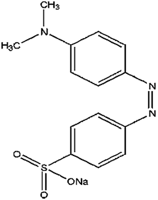 |
327.33 | — | 3.4 | 0.2 × 10³ |
| Eriochrome black T (EBT) | Naphthalenesulfonic acid, 3-hydroxy-4-[(1-hydroxy-2-naphthyl)azo]-7-nitro-, sodium salt |  |
461.37 | — | 6.2, 11.55 | 20 × 103 |
| Methylene blue (MB) | [7-(Dimethylamino)phenothiazin-3-ylidene]dimethylazanium; chloride | 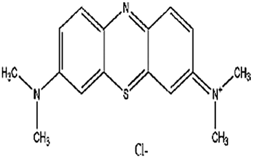 |
319.85 | 5.85 | 3.8 | 43.6 × 10³ |
| Crystal violet (CV) | Tris(4-(dimethylamino)phenyl)methylium chloride | 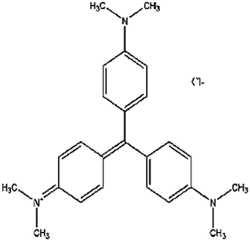 |
407.21 | 1.46 | 5.31, 8.64 | 4 × 10³ |
2. Experimental
2.1. Instrumentation
A UV-VIS spectrophotometer model AE-S90-MD form A & E Lab (UK) with 1 cm matched quartz cells was used for determination of dyes concentration. HPLC system model 1100 (Agilent Technologies, USA) with variable wavelength detector and an auto sampler was used for determination of dye mixtures.2.2. Reagents and materials
Ferric chloride (FeCl3), ferrous sulphate (FeSO4·7H2O), pectin from the rind of citrus or apple (galacturonic acid ≥ 74.0%) and tetraethoxysilane (TEOS) were purchased from Fisher Scientific (USA). Methyl orange (CI 13025, CAS 30065-G25, purity 85%) and Eriochrome black T (CI 14645, CAS 260320 G25, purity 85%) were supplied from S D Fine-Chem Ltd. (India). Mehtylene blue (CI 52015, CAS 61-73-4, purity 85%) was supplied from Muby chemicals (India) and crystal violet (CI 42535, CAS 548-62-9, purity 85%) was supplied from Lobachemie (India). HPLC grade acetonitrile and methanol were purchased from Fisher scientific (UK). Ammonium acetate was purchased from Sigma Aldrich (Germany). All other chemicals and reagents used were of analytical grade or higher. Ultra-pure water was obtained using a MilliQ UF-Plus system (Millipore, Eschborn, Germany) with a resistivity of at least 18.2 MΩ cm at 25 °C and TOC value below 5 ppb.2.3. Analysis techniques
Optimization and system suitability. HPLC chromatographic separation was achieved using a Thermo electron corporation Betasil C8 column (250 × 4.6 mm, 5 μm). Gradient elution using a mobile phase: (A) acetonitrile and (B) ammonium acetate buffer, pH 6.8 was achieved as follows: 0.0–5.5 min (40% A to 60% B, 1 mL min−1), 5.5–6.0 min (65% A to 35% B, 2 mL min−1), 6.0–7.0 min (85% A to 15% B, 2 mL min−1), 7.0–9.0 min (79% A to 21% B, 2 mL min−1), 9.0–11.0 min (60% A to 40% B, 2 mL min−1) and 11.0–13.0 min (40% A to 60%, 1 mL min−1). Analyses were performed at ambient temperature, detection was carried out at 520 nm and the injection volume was 20 μL.
Calibration and validation. Accurately measured aliquots of working standard solutions equivalent to (50–250 mg L−1) of each dye were separately transferred into a set of 25 mL volumetric flasks and then completed to volume with (1
:1 methanol:ammonium acetate buffer; pH 6.8). Analysis was carried out as described and the calibration curve for each compound was obtained by plotting area under the peak against concentration. Assay validation was carried out as per ICH guidelines.29–31
2.4. Preparation of modified magnetite nanoparticles
:1 molar ratio of ferric and ferrous ions was added drop wise into the pectin solution under vigorous mechanical stirring. The volume of solution was maintained at 300 mL and stirred for an additional 20 min. The ammonia solution (33 wt%) was then added drop wise till the solution became completely black indicating the formation of magnetite. The mixture was stirred for another 30 min and the black precipitate was collected, washed with distilled water, dried in the oven at 90 °C, and grinded with mortar.Preparation of MNPs via co-precipitation. The chemical co-precipitation method was employed to synthesize the MNPs. FeSO4·7H2O and FeCl3 (molar ratio, 1
:2) were dissolved in 20 mL distilled water and stirred for 20 min. NaOH solution (30 g%) was added drop wise under vigorous stirring until a dark colored precipitate was formed. The solution was then stirred for another 20 min under heating at 70 °C until the dark precipitate turned black. The particles were cooled to room temperature, magnetically decanted and washed several times with water.
Preparation of core–shell MS NPs. Following Stober process,33,34 a suspension of the synthesized magnetic nanoparticles (≈1.00 g) was diluted by a mixture of ethanol (80 mL) and water (18.5 mL). After addition of ammonia solution (0.5 mL, 33 wt%), TEOS (1 mL) was added to the reaction solution and mechanically stirred at 25 °C for 16 h. Silica was formed on the surface of magnetite nanoparticles through hydrolysis and condensation of TEOS. The formed MS NPs were then washed three times with deionized water and ethanol using external magnetic decantation.
Preparation of double shell MSP NPs. Pectin solutions of different concentrations (0.3, 0.5, 0.7 and 1% w/v) were prepared by dissolving 0.3 g, 0.5 g, 0.7 g and 1.0 g of pectin in 75 mL distilled water. The prepared solutions were then left under continuous stirring for 24 h at room temperature. Pectin solution was then added drop wise to a 25 mL suspension of the synthesized silica coated magnetic nanoparticles (≈1.00 g) and left stirring for 24 h. The mixture was collected by a permanent magnet, washed with distilled water and dried in the oven at 60 °C for 5 h.
2.5. Single dye adsorption experiments
The influence of pH on model dye removal was investigated using 100 mg L−1 of dyes solutions over pH range of 2.0–8.0. The pH was adjusted by adding aqueous solutions of 0.1 mol L−1 HCl or 0.1 mol L−1 NaOH. To each of the pH-adjusted dye solution, 2 g L−1 of the adsorbents were added and shaken for 120 min at 25 °C.
To study the effect of adsorbents concentration 0.5, 1.0, 2.0, 3.0, 4.0 and 5.0 g L−1 of both adsorbents were added to 50 mL dye solutions (100 mg L−1) with contact time of 120 min. The pH was adjusted at pH 2.0 for anionic dyes and pH 8.0 for cationic dyes. Adsorption capacities were then determined for each adsorbent concentration to determine the optimal concentration of adsorbent that cause complete dye removal.
2.6. Desorption experiment
Recovery of model dyes (MB and EBT) from dye-loaded MP NPs and dye-loaded MSP NPs was performed by initially conducting adsorption experiments with a mixture of 100 mg L−1 dyes solutions and 2 g L−1 of both adsorbents for 120 min. After equilibrium, the dye-loaded NPs were magnetically separated and the supernatant was measured for dye concentration to estimate the amount of dye adsorbed on adsorbent NPs. The dye-loaded NPs were then shaken separately with 50 mL of 5% (v/v) methanol and acetic acid (96%) for 1 h in case of cationic dye (MB) and 50 mL methanol and 50 mL of 5% (v/v) methanol and NaOH in case anionic dye (EBT). The adsorbent was collected by a magnet and reused for adsorption again. The supernatant solutions were analyzed by UV-VIS spectrophotometry to determine the amount of released dye. The cycles of adsorption–desorption processes were successively conducted three times.2.7. Dye mixture adsorption experiments
Adsorption experiments were carried out in a batch mode by taking 50 mL of the model dyes (MO, EBT, MB and CV) solution mixture containing 165 mg L−1 of each dye in 250 mL Erlenmeyer flask. The influence of pH on model dyes removal was investigated over a pH range (2–8) to investigate the efficiency of MP NPs and MSP NPs for selective adsorption of cationic (MB and CV) and anionic (MO and EBT) dyes. The pH was adjusted by adding aqueous solutions of 0.1 mol L−1 HCl or 0.1 mol L−1 NaOH to the model dyes working solutions. Then to each of the pH-adjusted dyes mixture solutions, 2 g L−1 of MP and MSP NPs were added separately and shaken at 25 °C with a speed of 240 rpm. After 2 h samples were removed and the concentration of dyes left in the supernatant solutions after magnetic separation were determined using the HPLC proposed assay. A quantitative determination of dye concentration was achieved by using the linear regression equations, obtained from the calibration curve prepared with a range of dye concentration (50–250 mg L−1).2.8. Data analyses and modeling
The amount of dye adsorbed at time t, qt and at equilibrium, qe, was calculated using the mass balance equation qt = (C0 − Ct) (V m−1), where C0 and Ct (mg L−1) are the initial and final dye concentrations, respectively, V (L) is the volume of the dye solution and m (g) is the mass of adsorbent. When t is equal to the equilibrium time, that is Ct = Ce, qt = qe, then qe can be calculated using the same equation as given above. The amount of dyes removed at various solution pH was expressed in percentage (R, %) and calculated using the equation| R = 100(C0 − Ce)/C0 |
2.9. Statistical analysis
Since error functions are required to assess the kinetic and isotherm models describing the experimental results in a best possible way, the R2 and chi-square tests are performed to find out the suitability of various kinetic and isotherm models in the present study.35where, qe,exp and qe,cal (mg g−1) are experimental and calculated dye concentration at equilibrium, respectively and qe,cal (mg g−1) is average value of qe,cal.
3. Results and discussion
3.1. Analysis techniques
| Item | MO | EBT | MB | CV |
|---|---|---|---|---|
| Wavelength of detection | 465 nm | 531 nm | 663 nm | 585 nm |
| Range of linearity | 1.5–30 μg mL−1 | 3–30 μg mL−1 | 0.75–12 μg mL−1 | 1.5–21 μg mL−1 |
| Regression equation | A = 0.0723C − 0.0172 | A = 0.0279C + 0.0024 | A = 0.1754C + 0.0575 | A = 0.1053C + 0.0122 |
| Regression coefficient (r2) | 0.9999 | 0.9999 | 0.9999 | 0.9998 |
| LOD (μg mL−1) | 0.22 | 0.55 | 0.12 | 0.21 |
| LOQ (μg mL−1) | 0.65 | 1.67 | 0.36 | 0.63 |
| SD of slope-Sb | 0.0004 | 0.0002 | 0.0008 | 0.0008 |
| SD of intercept-Sa | 0.008 | 0.003 | 0.005 | 0.01 |
| Accuracy mean ± SD | 99.76 ± 0.56 | 99.59 ± 0.87 | 100.71 ± 0.79 | 100.14 ± 0.94 |
| Repeatability (% RSD, n = 6) | 0.51 | 1.28 | 0.44 | 0.77 |
| Precision | ||||
| Intraday % RSD (n = 3) | 0.17–0.23 | 0.09–0.1 | 0.07–1.03 | 0.03–0.59 |
| Interday % RSD (n = 3) | 0.14–1.01 | 0.64–1.44 | 0.59–1.02 | 0.43–1.2 |
The retention times were 4.4, 5.1, 5.6 and (7.9, 8.6 and 9.2) min for MO, EBT, MB and CV respectively; as shown in Fig. S1[a–d].† Good resolution and absence of interference between the dyes being analyzed are shown in Fig. 1.
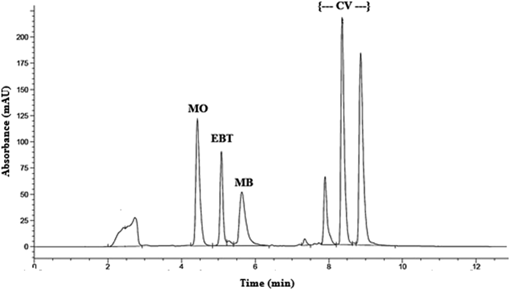 | ||
| Fig. 1 HPLC chromatogram of model dyes: methyl orange (MO), Eriochrome black T (EBT), methylene blue (MB) and crystal violet (CV). | ||
Peak purity test showed that the peaks having retention times at (7.9, 8.6 and 9.2) min all belong to crystal violet and most probably to its demethylated forms. According to the study of Confortin et al. demethylation causes a blue shift in the absorption spectra and a decrease in retention time.36 Thus it is expected that the peaks at 7.9, 8.6 and 9.2 min are for crystal violet, mono-demethylated crystal violet and di-demethylated crystal violet respectively. In addition, the chromatograms of the dyes in the sample solutions were found identical to the chromatograms received by the standard solutions at the wavelength applied.
System suitability parameters were calculated according to The United States Pharmacopoeia and National Formula and The WHO International Pharmacopoeia,37,38 and separation efficiency was demonstrated (Table 3). Method validation was carried out according to ICH guidelines.29–31 Regression equation and validation parameters are summarized in Table 4.
| Parameters | Obtained value | Reference value37,38 | |||
|---|---|---|---|---|---|
| MO | EBT | MB | CV | ||
| Retention time (tR) | 4.43 | 5.08 | 5.64 | 7.90 | |
| Symmetry factor (As) | 1 | 1.1 | 1.5 | 1.5 | T ≤ 2 |
| Theoretical plates number (N) | 9151 | 22062 |
5650 | 46640 |
N ≥ 2000 |
| Capacity factor (k) | 1 | 1.3 | 1.6 | 2.6 | 1–10 acceptable |
| Resolution (Rs) | 2.38 | 1.51 | 5.97 | — | Rs ≥ 1.5 |
| Selectivity factor (α) | 1.29 | 1.20 | 1.66 | — | α > 1 |
| Item | MO | EBT | MB | CV |
|---|---|---|---|---|
| Retention time | 7.90 | 5.64 | 5.08 | 4.43 |
| Wavelength of detection | 520 nm | 520 nm | 520 nm | 520 nm |
| Range of linearity | 50–250 μg mL−1 | 50–250 μg mL−1 | 50–250 μg mL−1 | 50–250 μg mL−1 |
| Regression equation | A = 14.239C + 8.3887 | A = 18.502C + 8.6695 | A = 11.702C + 23.923 | A = 39.749C + 65.485 |
| Regression coefficient (r2) | 0.9997 | 0.9997 | 0.9995 | 1 |
| LOD (μg mL−1) | 2.47 | 1.70 | 2.80 | 3.22 |
| LOQ (μg mL−1) | 7.47 | 5.14 | 8.47 | 9.76 |
| SD of slope-Sb | 0.114 | 0.163 | 0.129 | 0.106 |
| SD of intercept-Sa | 18.960 | 27.545 | 21.517 | 17.636 |
| Accuracy mean ± SD | 99.62 ± 1.03 | 100.72 ± 1.16 | 101.04 ± 0.69 | 101.12 ± 0.89 |
| Repeatability (% RSD, n = 6) | 0.75 | 0.51 | 1.2 | 1.38 |
| Precision | ||||
| Intraday % RSD (n = 3) | 0.07–0.16 | 0.22–1.43 | 0.99–1.34 | 0.3–1.02 |
| Interday % RSD (n = 3) | 1.08–1.53 | 0.4–1.98 | 0.82–1.34 | 0.65–1.55 |
3.2. Characterization of the prepared nanoparticles
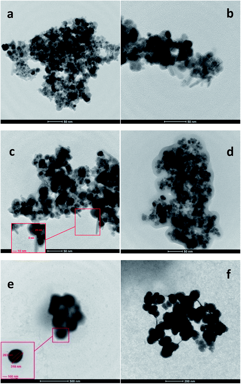 | ||
| Fig. 2 TEM image of; [a] MNPs, [b] MS NPs, [c] MSP NPs (0.5 w/v%), [d] MSP NPs (1 w/v%), [e] MP NPs (0.5 w/v%), [f] MP NPs (1 w/v%). Magnetite Nanoparticles: MNPs; Magnetite/Silica Nanoparticles: MS NPs; Magnetite/Pectin Nanoparticles: MP NPs and Magnetite/Silica/Pectin Nanoparticles: MSP NPs. | ||
TEM analysis of the MP NPs demonstrates that the presence of pectin during the formation of MNPs increases the size of magnetite nanoparticles. However, to a great extent pectin prevented particle aggregation due to the dispersion of magnetite within pectin matrix. Fig. 2[e] shows the MP (0.5 w/v%) nanoparticles with a diameter range of 200–500 nm. On the other hand, Fig. 2[f] illustrates the MP NPs (1 w/v%) ranging from 50 to 100 nm in diameter. Such difference in size of the coated samples indicates that the coating material has an effect on the size of particles which comes in agreement with what was mentioned in previous studies.39 Having a close look at Fig. 2[e] and [f], the light atoms of carbon, hydrogen and oxygen, which constitute the polysaccharide structure of pectin, correspond to brightest areas. The heavy Fe atom allows a better contrast and corresponds to darkest areas which are scattered as dots within the pectin matrix. In addition, these TEM images show some level of aggregation and non-uniform coating of the MNPs. Nevertheless, there is some improvement in the dispersion of iron oxide particles in pectin matrix than the pure magnetite nanoparticles. Thus it can be concluded that both types of nanoparticles enhanced the dispersion of the MNPs yet the control of particles size in case of MSP NPs was better than that of MP NPs.
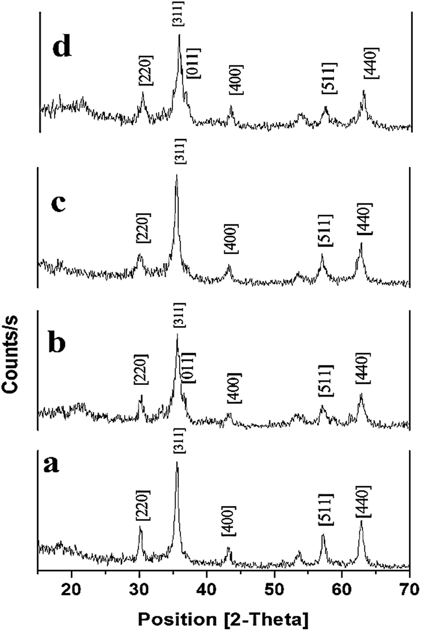 | ||
| Fig. 3 XRD pattern of; [a] MNPs, [b] MS NPs, [c] MP (0.5 w/v%) NPs, and [d] MSP (0.5 w/v%) NPs. Magnetite Nanoparticles: MNPs; Magnetite/Silica Nanoparticles: MS NPs; Magnetite/Pectin Nanoparticles: MP NPs and Magnetite/Silica/Pectin Nanoparticles: MSP NPs. | ||
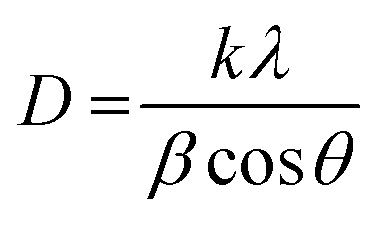
The intensity of the peaks corresponding to the surface functional groups was found to be reduced upon using pectin and silica. This reduction for MSP NPs is more than that of MP NPs due to the double shell property of the former. The crystal sizes of the hybrid NPs were also determined from the XRD pattern by using Scherrer's equation;6
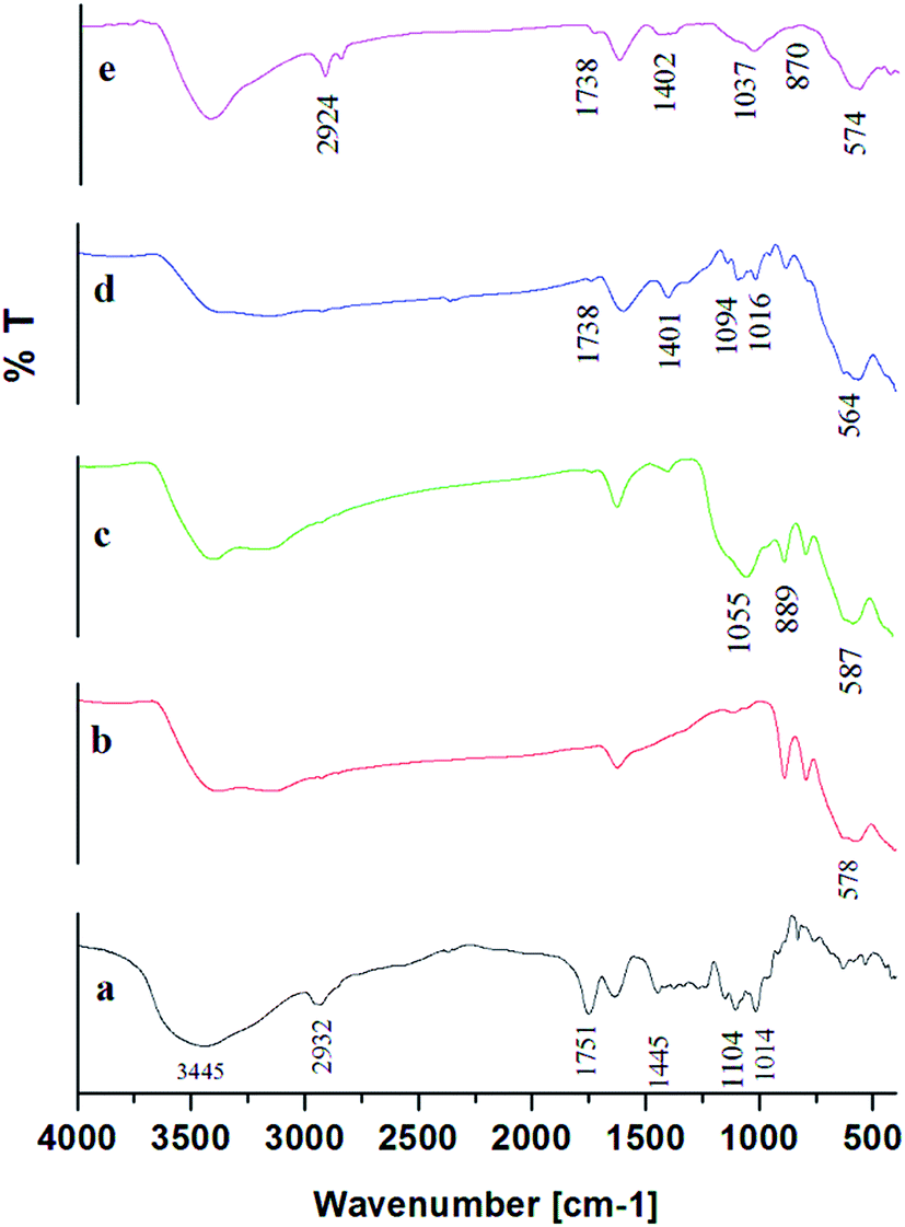 | ||
| Fig. 4 FTIR data for; [a] pure pectin, [b] MNPs, [c] MS NPs, [d] MP (0.5 w/v%) NPs pectin, and [e] MSP (0.5 w/v%) NPs. Magnetite Nanoparticles: MNPs; Magnetite/Silica Nanoparticles: MS NPs; Magnetite/Pectin Nanoparticles: MP NPs and Magnetite/Silica/Pectin Nanoparticles: MSP NPs. | ||
The characteristic vibration bands of SiO2 as listed in literature are mainly: νas(Si–O–Si) at 1200 cm−1 and 1075 cm−1; νas(Si–OH) at 970 cm−1; νs(Si–O–Si) at 795 cm−1; ν(Si–O–Si) from cyclic tetramers at 540 cm−1 and δ(Si–O–Si) at 460 cm−1.43 Noticeably, in Fig. 4[c] representing MS NPs, the absorption of SiO2 was confirmed by the shift of the νas(Si–OH) peak at 1037 cm−1 and Si–O–Si bond shift at 889 cm−1 indicating that iron ions might be bonded to silicate skeleton through O–Si–O–Fe–O–Si–O linkage.34,43,44 (Si–OH) and Si–O–Si peaks also appeared in the MSP NPs in the range 1044–1055 cm−1 and 867–889 cm−1 respectively. Such findings illustrate the specific interactions between MNPs and silica which can be covalent, through Si–O–Fe bond formation; electrostatic, between negatively charged Si–O terminal ligands and positively charged groups on the particle surface; or hydrogen-bond interactions between hydration layers of silanol groups and the particle surface.45
Furthermore, there was a disappearance of the peaks 1014 and 1095 cm−1 from the MSP NPs spectra (Fig. 4[e] for 0.5 w/v% pectin, and Fig. S5† for 0.3, 0.7 and 1 w/v% pectin) which correspond to the vibrations associated with the skeletal rings of the sugar monomers of pectin and C–OH of alcoholic groups respectively.32 Such finding can be attributed to the overlapping of OH groups of sugar monomers with the Si–O band of the silica stabilization.32,44 The appearance of peaks at 1737–1739 cm−1 and 1402–1408 cm−1 assigned to the stretching vibrations of C–O and carboxylic acids in ionic form (COO−) respectively, indicates the successful binding of pectin onto the MS NPs.32,42
 | ||
| Fig. 5 Hysteresis loop of NPs of; [a] MNPs, [b] MS NPs, [c] MP NPs (0.5 w/v%) pectin, and [d] MSP NPs (0.5 w/v%) pectin. Magnetite Nanoparticles: MNPs; Magnetite/Silica Nanoparticles: MS NPs; Magnetite/Pectin Nanoparticles: MP NPs and Magnetite/Silica/Pectin Nanoparticles: MSP NPs. | ||
Notably, the saturation magnetization measured in most of our coated NPs was acceptable for potential magnetic separation because Ms of 16.3 emu g−1 was sufficient for magnetic separation with a conventional permanent magnet.47 Compared with MNPs, the saturation magnetization decreased in both types of coated NPs which could be due to the formation of magnetic dead layer by non-magnetic material (pectin) at the domain boundary wall of Fe3O4 NPs.48 Nevertheless, MSP NPs (0.3 w/v% and 0.5 w/v%) showed a greater decrease in saturation magnetization than MP NPs (0.3 w/v% and 0.5 w/v%). Such decrease could be related to the formation of an additional non-magnetic layer of silica in MSP NPs.
It is also worth mentioning that the saturation magnetization of coated samples decreased with increasing pectin concentration. Such result can be attributed to the decrease in the amount of MNPs for the same volume of measured samples and thus affect their total magnetic moment. However, despite the increase in pectin concentration the MSP was able to maintain a favorable range of Ms values than the MP NPs. A significant decrease in the Ms of MP NPs (0.7 w/v% and 1 w/v%) reaching 12 and 5 emu g−1 respectively was observed and could be due to the formation of goethite phase in the NPs which has decreased Ms than that of magnetite.18
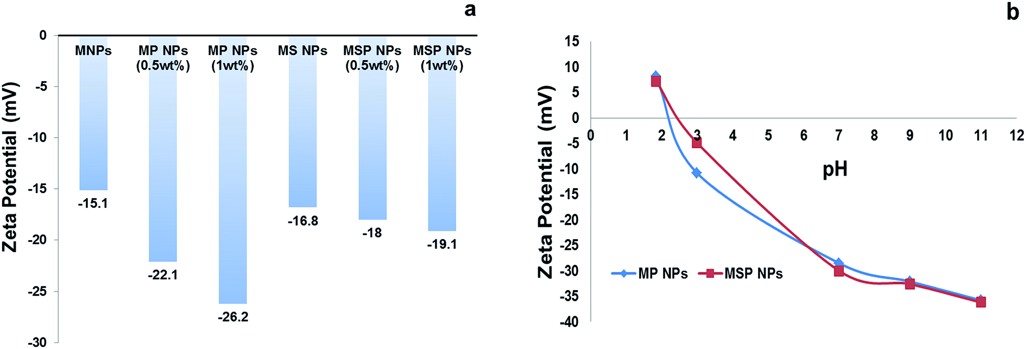 | ||
| Fig. 6 Zeta potential of the nanoparticles; [a] at neutral pH and [b] at different pH. | ||
The pHzpc of MP NPs and MSP NPs is found to be 2.2 and 2.5 respectively as illustrated in Fig. 6[b], which compares well with those reported previously for magnetite NPs coated with pectin.32 Thus, the surface both types of adsorbents will be either positively or negatively charged at pH < 2.5 or pH > 2.5, respectively, which entails the advantage of removal of anionic or cationic dyes from water via adsorption at different pH levels.
3.3. Single dye adsorption experiments
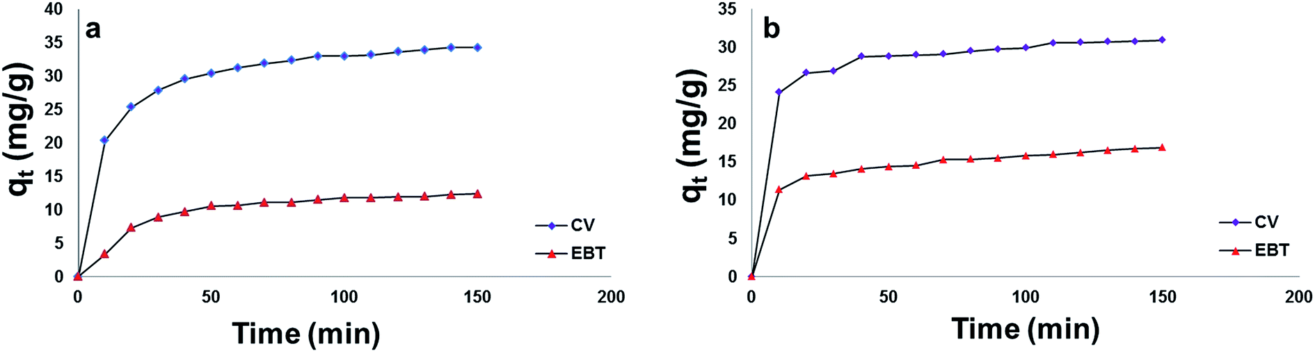 | ||
| Fig. 7 Effect of contact time on the adsorption capacity (qt) of EBT and CV onto; [a] MSP NPs and [b] MP NPs. Adsorbent: 2 g L−1, dyes 100 mg L−1, temperature: 25 °C, pH: natural pH of dye, time: 150 min. Magnetite/Pectin Nanoparticles: MP NPs and Magnetite/Silica/Pectin Nanoparticles: MSP NPs. | ||
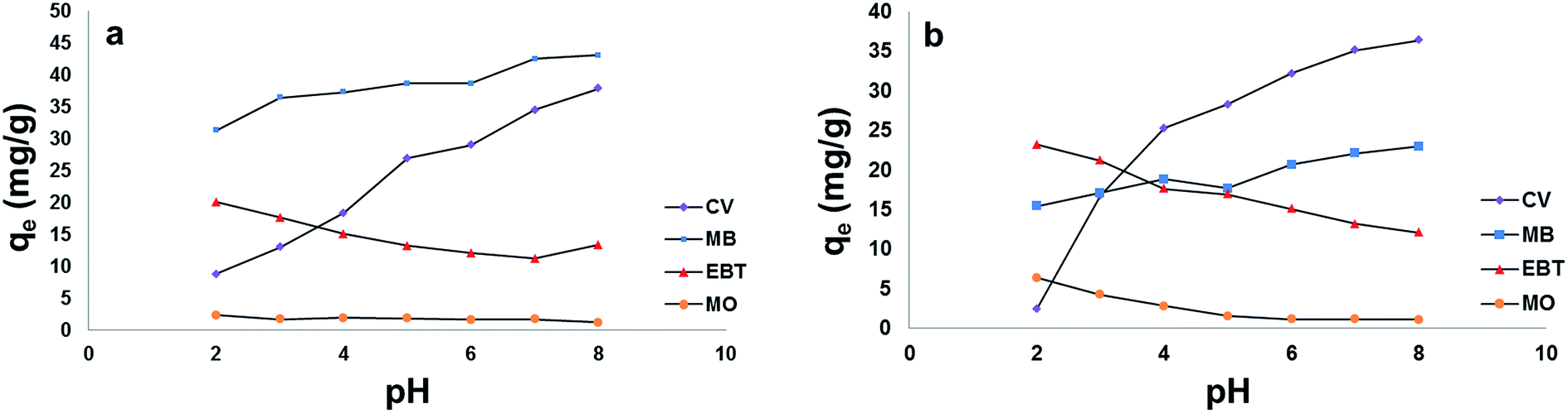 | ||
| Fig. 8 Effect of pH on the adsorption capacity (qe) of model dyes onto; [a] MSP NPs and [b] MP NPs. Adsorbent: 2 g L−1, dyes 100 mg L−1, temperature: 25 °C, time: 120 min. Magnetite/Pectin Nanoparticles: MP NPs and Magnetite/Silica/Pectin Nanoparticles: MSP NPs. | ||
For the anionic dyes (MO and EBT), as observed in Fig. 8[a] and [b], the adsorption is high in acidic medium and decreases with the increase in solution pH. This can be attributed to the fact that as the pH is lowered, the hydroxyl and carboxylic groups of pectin are protonated and the overall surface charge on the NPs will become positive. Such result will promote reaction with EBT and MO as anionic dyes through electrostatic forces of attraction.
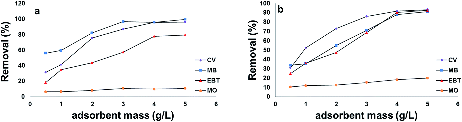 | ||
| Fig. 9 Effect of adsorbent mass on the removal efficiency of model dyes onto: [a] MSP NPs and [b] MP NPs. Dyes 100 mg L−1, temperature: 25 °C, pH: 2.0 for anionic dyes and 8.0 for cationic dyes, time: 120 min. Magnetite/Pectin Nanoparticles: MP NPs and Magnetite/Silica/Pectin Nanoparticles: MSP NPs. | ||
On the other hand, an increase in cationic dyes – CV and MB – adsorption took place at pHs above the pHzpc of both types of NPs due to the electrostatic attraction between negatively charged sites on the adsorbents and dyes cations. The ionic nature of the two basic dyes (methylene blue and crystal violet) could have played a role in retaining the dye species on the surface of the adsorbents. The molecular structure of methylene blue has ionic charge, with decentralised or delocalised positive charge on its organic structure. Similar arguments could be applied to the structure of crystal violet.57
A superior adsorption of cationic dyes on MSP NPs was observed than that on MP NPs while it was the opposite for anionic dyes adsorption. This can be attributed to the presence of an additional silica shell in MSP NPs which offers more negative charge on the surface than MP NPs at elevated pHs. Such condition favors the electrostatic attraction between the negatively charged silanol groups (Si–O) on NPs surface and the positively charged cationic dyes monomers to form a strong hydrogen bond and increasing their adsorption capacity.58 In addition, MB showed higher adsorption capacity than that of CV on MSP NPs and this might be due to the affinity of MB to the silica shell of MP NPs than that of CV. On the other hand, since the MP NPs offers a lesser negatively charged surface than MSP NPs in acidic pH, it favors the adsorption of anionic dyes than that of MSP NPs.
 | (1) |
After linearization of the Langmuir isotherm, eqn (2), we obtain:
 | (2) |
The values of Q0 and b are calculated from the slope and intercept of the plot of Ce/qe vs. Ce for MSP NPs and MP NPs (Fig. S8†).
The Freundlich isotherm model is an empirical equation that describes the surface heterogeneity of the sorbent. It considers multilayer adsorption with a heterogeneous energetic distribution of active sites, accompanied by interactions between adsorbed molecules.60 The Freundlich empirical model is represented by:
| qe = KfCe1/n | (3) |
 | (4) |
The values of Kf (mL g−1) and 1/n are calculated from the intercept and slope of the plot of lnqe vs. lnCe for MSP NPs and MP NPs (Fig. S9†).
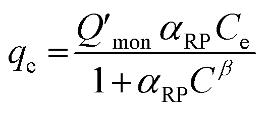
The Redlich–Peterson isotherm unites the Langmuir and Freundlich isotherms, it describes adsorption on heterogeneous surfaces, as it contains the heterogeneity factor β. This equation has three parameters, KRP is the constant of Redlich–Peterson isotherm (mL g−1), αRP is the Redlich–Peterson constant (mL mg−1), and β is the Redlich–Peterson exponent (0 < β < 1). It can be reduced to the Langmuir equation as β approaches 1.61,64 The general equation can be described as follows61,65
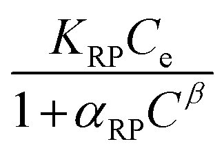 | (5) |
 | (6) |
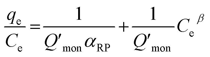
According to Wu et al.,65 a linear form of eqn (6) can be transformed as
 | (7) |
The Redlich–Peterson isotherm curves of the model dyes are presented in Fig. S10† using the plot of qe/Ce vs. Ceβ for MSP NPs and MP NPs.
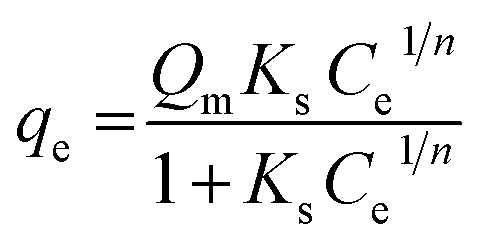
Sips developed a new model as an improvement to the Freundlich and Langmuir equations.66 This model is based on the Freundlich equation assumption, where the amount of adsorbed dye increases with the increase of initial concentration, but Sips equation presumes that the adsorption capacity has a finite limit when the concentration is sufficiently high.67 The Sips62 equation can be represented as follows;
 | (8) |
The Sips isotherm curves of the model dyes are presented in Fig. S11† using the plot of qe vs. Ce1/n for MSP NPs and MP NPs.
The parameters of Langmuir, Freundlich, Redlich–Peterson and Sips equations are listed in Table 5 for MSP and MP NPs. For both of MSP and MP NPs, the values of correlation coefficient, R2, and Chi square (χ2) for the fit of experimental isotherm data to equation are the best for Sips model. Such results indicate that the adsorption process of model dyes is going on after a combined model Freundlich and Langmuir: diffused adsorption on low dye concentration, and a monomolecular adsorption with a saturation value at high adsorbate concentrations.66,68,69 Additionally, the values of 1/n for Sips isotherm are 0 < 1/n < 1, indicating that the dyes adsorption process is favorable.
| Langmuir | Freundlich | Redlich-Peterson | Sips | ||||||||||||||||
|---|---|---|---|---|---|---|---|---|---|---|---|---|---|---|---|---|---|---|---|
| Q0 (mg g−1) | B (mL mg−1) | RL | R2 | χ2 | Kf (mL g−1) | 1/n | R2 | χ2 | KRP × 103 (mL g−1) | αrp (mL mg−1) | β | R2 | χ2 | Qm (mg g−1) | Ks (mL mg−1) | 1/n | R2 | χ2 | |
| MSP NPs | |||||||||||||||||||
| CV | 125 | 16 | 0.2336 | 0.9922 | 0.505 | 328.09 | 0.648 | 0.9908 | 1.854 | 2 | 12.8 | 0.8648 | 0.9965 | 0.4235 | 180.295 | 1.949 | 0.6547 | 0.9987 | 0.145 |
| MB | 185.18 | 27 | 0.1583 | 0.9974 | 3.888 | 650.018 | 1.625 | 0.9657 | 7.342 | 10 | 46 | 0.9142 | 0.9984 | 0.2817 | 197.18 | 2.512 | 0.5578 | 0.9971 | 0.365 |
| EBT | 108.69 | 10.22 | 0.3318 | 0.8132 | 0.816 | 219.79 | 0.6268 | 0.9922 | 0.231 | 2.5 | 12.25 | 0.5281 | 0.9232 | 1.7076 | 65.35 | 3.849 | 0.6688 | 0.9929 | 0.655 |
| MO | 60.61 | 3.75 | 0.5727 | 0.7382 | 0.638 | 102.74 | 0.8136 | 0.992 | 0.470 | 1.11 | 11.66 | 0.1614 | 0.8252 | 0.4702 | 26.754 | 3.277 | 0.7277 | 0.992 | 0.4704 |
|
|||||||||||||||||||
| MP NPs | |||||||||||||||||||
| CV | 100 | 25 | 0.1632 | 0.9965 | 0.881 | 265.52 | 0.5923 | 0.9795 | 3.252 | 2.5 | 18.5 | 0.8196 | 0.9935 | 0.8168 | 140.49 | 2.085 | 0.425 | 0.9973 | 0.2139 |
| MB | 92.59 | 36 | 0.1173 | 0.9929 | 1.468 | 210.44 | 0.4746 | 0.9797 | 2.686 | 10 | 70 | 0.7241 | 0.993 | 1.357 | 168.72 | 1.036 | 0.6021 | 0.9897 | 0.599 |
| EBT | 133.33 | 10.71 | 0.3149 | 0.883 | 2.947 | 297.56 | 0.6567 | 0.9954 | 0.726 | 2 | 8.8 | 0.6353 | 0.9485 | 1.4 | 72.348 | 3.212 | 0.579 | 0.9925 | 0.839 |
| MO | 126.58 | 2.82 | 0.6392 | 0.6091 | 1.085 | 183.48 | 0.8415 | 0.9947 | 0.576 | 0.37 | 2.296 | 0.8061 | 0.6645 | 0.9687 | 27.215 | 4.3837 | 0.708 | 0.9945 | 0.445 |
The Qm values were calculated form the Sips isotherm for cationic dyes at optimum pH (∼8) for MP and MSP NPs and were estimated to be (CV = 140.49 mg g−1, MB = 168.72 mg g−1) and (CV = 180.29 mg g−1, MB = 197.18 mg g−1), respectively. For the anionic dyes, the Qm values calculated at optimum pH (∼2) for MP and MSP NPs were estimated to be (EBT = 72.35 mg g−1, MO = 27.215 mg g−1) and (EBT = 65.35 mg g−1, MO = 2 6.754 mg g−1), respectively. This data indicates that our proposed adsorbents (MSP NPs and MP NPs) can be considered promising materials for the removal of cationic and anionic dyes from aqueous solution.
Generally, isotherms relating solid-phase to fluid-phase concentration for adsorption of a single component directly influence the behavior of the isotherm curves.70 The elucidation relating the isotherm curves and the equilibrium behavior is given by a dimensionless “separation factor” or “equilibrium parameter”, (RL) which is presented by eqn (9):
| RL = 1/(1 + bC0) | (9) |
| Sorbent | Capacity factor (Q0 (mg g−1)) | Kinetic models | Ref. | |||
|---|---|---|---|---|---|---|
| CV | MB | EBT | MO | |||
| Fe3O4@APS@AA-co-CA MNPs | 208 | 142.9 | — | — | Pseudo 2nd order | 71 |
| Magnetic-modified multi-walled carbon nanotubes | 227 | 48.1 | — | — | — | 72 |
| Magnetic nanocomposite | 81 | — | — | — | — | 73 |
| MWCNTs/Mn0.8Zn0.2Fe2O4 composite | 5 | — | — | — | Pseudo 2nd order | 74 |
| N-Benzyl-O-carboxymethylchitosan magnetic NPs | 248 | 223.58 | — | — | Pseudo 2nd order | 54 |
| Magnetite nanoparticles loaded tea waste (MNLTW) | 113.69 | 119 | — | — | Pseudo 2nd order | 75 |
| Graphene nanosheet (GNS)/magnetite (Fe3O4) composite | — | 43.82 | — | — | Pseudo 2nd order | 76 |
| Poly(c-glutamic acid) (PGA-MNPs) | — | 78.67 | — | — | Pseudo 2nd order | 5 |
| Montmorillonite clay modified with iron oxide (MtMIO) | — | 71.2 | — | — | Pseudo 2nd order | 77 |
| Fe3O4 NPs coated with pectin and crosslinked with adipic acid (FN-PAA) | — | 221.7 | — | — | Pseudo 2nd order | 6 |
| Eucalyptus bark | — | — | 52.37 | — | Pseudo 1st order | 78 |
| Scolymus hispanicus L. | — | 237.18 | 120.42 | — | Pseudo 2nd order | 79 |
| NiFe2O4 nanoparticles | — | — | 47 | — | Pseudo 2nd order | 80 |
| Nteje clay | 16.26 | Pseudo 2nd order | 81 | |||
| Activated carbon modified by silver nanoparticles | — | — | — | 0.69 | Pseudo 2nd order | 82 |
| Ash Moringa peregrina | — | — | — | 15.43 | — | 83 |
| Dragon fruit (Hylocereusundatus) foliage | — | — | — | 17.67 | Pseudo 2nd order | 84 |
| Chitosan intercalated montmorillonite | — | — | — | 70.42 | Pseudo 2nd order | 85 |
| Silica gel waste (SGW), modified with cationic surfactant | — | — | — | 45.45 | Pseudo 2nd order | 86 |
| Polyaniline modified ZnO | — | — | — | 28.94 | Pseudo 1st order | 87 |
| Magnetite/pectin NPs | 100 | 125 | 103.41 | 47.36 | Pseudo 2nd order | Present work |
| Magnetite/silica/pectin NPs | 125 | 178.57 | 80.15 | 27.74 | Pseudo 2nd order | Present work |
 | (10) |
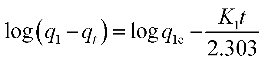
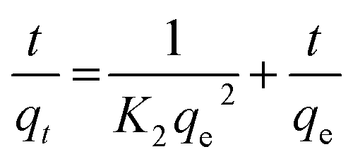
Ho and McKay90 presented the pseudo-second order kinetic as:
 | (11) |
Fig. S12 and S13† are the plots of the pseudo-first order and second order kinetics of model dyes adsorption on MSP respectively. Fig. S15 and S16† are the plots of the pseudo-first order and second order kinetics of model dyes adsorption on MP NPs respectively. The calculated kinetic parameters are given in Tables 7 and 8 for MSP NPs and MP NPs respectively.
| Pseudo 1st order | Pseudo 2nd order | Intraparticle diffusion | |||||||||||
|---|---|---|---|---|---|---|---|---|---|---|---|---|---|
| qe (exp) (mg g−1) | qe (cal) (mg g−1) | K1 (h−1) | R2 | χ2 | qe (cal) (mg g−1) | K2 (mg g−1 h−1) | R2 | χ2 | Kid | C | R2 | χ2 | |
| CV | |||||||||||||
| 10 mg L−1 | 9.94 | 5.93 | 2.612 | 0.9308 | 0.252 | 10.56 | 0.760 | 0.9976 | 0.207 | 0.376 | 6.174 | 0.8918 | 0.138 |
| 50 mg L−1 | 36.51 | 10.15 | 1.912 | 0.9311 | 0.039 | 37.45 | 0.419 | 0.9997 | 0.118 | 0.878 | 27.563 | 0.8865 | 0.205 |
| 100 mg L−1 | 64.94 | 14.87 | 2.501 | 0.949 | 0.129 | 66.23 | 0.380 | 0.9998 | 0.175 | 1.047 | 54.551 | 0.8459 | 0.222 |
| 150 mg L−1 | 78.61 | 15.74 | 1.275 | 0.9701 | 0.058 | 80 | 0.195 | 0.9992 | 1.374 | 1.563 | 61.505 | 0.9705 | 0.067 |
| 200 mg L−1 | 90.29 | 31.12 | 2.873 | 0.9669 | 0.081 | 93.46 | 0.164 | 0.9998 | 0.243 | 2.389 | 67.356 | 0.843 | 0.857 |
|
|||||||||||||
| MB | |||||||||||||
| 10 mg L−1 | 12.84 | 2.89 | 3.195 | 0.9756 | 0.026 | 13.09 | 2.335 | 0.9998 | 0.049 | 0.194 | 10.988 | 0.7994 | 0.051 |
| 50 mg L−1 | 66.07 | 12.24 | 1.137 | 0.9607 | 0.202 | 66.67 | 0.25 | 0.9992 | 0.533 | 1.338 | 51.386 | 0.9089 | 0.207 |
| 100 mg L−1 | 107.58 | 23.65 | 1.928 | 0.9615 | 0.107 | 109.89 | 0.166 | 0.9998 | 1.111 | 1.889 | 88.125 | 0.9435 | 0.145 |
| 150 mg L−1 | 132.61 | 27.44 | 1.688 | 0.7998 | 0.498 | 135.14 | 0.137 | 0.9993 | 2.895 | 1.982 | 110.85 | 0.9722 | 0.061 |
| 200 mg L−1 | 151.16 | 40.5 | 2.004 | 0.9277 | 0.356 | 153.85 | 0.106 | 0.9996 | 1.18 | 3.469 | 116.06 | 0.8559 | 0.999 |
|
|||||||||||||
| EBT | |||||||||||||
| 10 mg L−1 | 9.23 | 10.23 | 2.553 | 0.8951 | 2.073 | 10.41 | 0.368 | 0.9977 | 0.123 | 0.571 | 3.423 | 0.9572 | 0.146 |
| 50 mg L−1 | 29.22 | 18.06 | 2.444 | 0.9728 | 0.148 | 31.25 | 0.233 | 0.9997 | 0.062 | 11.336 | 16.048 | 0.8601 | 0.843 |
| 100 mg L−1 | 38.64 | 19.25 | 2.225 | 0.9648 | 0.479 | 40.98 | 0.198 | 0.9993 | 0.146 | 1.674 | 22.213 | 0.8005 | 1.534 |
| 150 mg L−1 | 59.64 | 23.05 | 1.951 | 0.9715 | 1.627 | 62.5 | 0.151 | 0.9995 | 0.431 | 2.39 | 36.025 | 0.7583 | 2.605 |
| 200 mg L−1 | 76.09 | 26.47 | 1.56 | 0.9557 | 0.093 | 78.74 | 0.124 | 0.9989 | 1.112 | 2.393 | 50.712 | 0.9596 | 0.254 |
|
|||||||||||||
| MO | |||||||||||||
| 10 mg L−1 | 2.19 | 2.95 | 2.313 | 0.9221 | 1.58 | 2.77 | 0.695 | 0.9994 | 0.002 | 0.188 | 0.276 | 0.9653 | 0.064 |
| 50 mg L−1 | 9.26 | 5.28 | 1.796 | 0.9499 | 0.078 | 9.91 | 0.583 | 0.9979 | 0.226 | 0.422 | 4.831 | 0.9777 | 0.038 |
| 100 mg L−1 | 13.54 | 5.95 | 1.953 | 0.9632 | 0.075 | 14.39 | 0.525 | 0.9992 | 0.104 | 0.589 | 7.659 | 0.8898 | 0.247 |
| 150 mg L−1 | 22.46 | 10.46 | 2.011 | 0.9618 | 0.101 | 23.58 | 0.367 | 0.9992 | 0.255 | 0.804 | 14.213 | 0.9445 | 0.138 |
| 200 mg L−1 | 25.78 | 10.39 | 2.047 | 0.9905 | 0.249 | 27.03 | 0.351 | 0.9999 | 0.014 | 0.997 | 15.932 | 0.824 | 0.679 |
| Pseudo 1st order | Pseudo 2nd order | Intraparticle diffusion | |||||||||||
|---|---|---|---|---|---|---|---|---|---|---|---|---|---|
| qe (exp) (mg g−1) | qe (cal) (mg g−1) | K1 (h−1) | R2 | χ2 | qe (cal) (mg g−1) | K2 (mg g−1 h−1) | R2 | χ2 | Kid (mg g−1 min−0.5) | C (L) | R2 | χ2 | |
| CV | |||||||||||||
| 10 mg L−1 | 10.46 | 5.81 | 1.865 | 0.9747 | 0.039 | 11.22 | 0.526 | 0.9994 | 0.036 | 0.514 | 5.22 | 0.9107 | 0.221 |
| 50 mg L−1 | 37.59 | 7.32 | 1.349 | 0.9365 | 0.091 | 38.17 | 0.458 | 0.9995 | 0.202 | 0.782 | 29.279 | 0.983 | 2.058 |
| 100 mg L−1 | 62.49 | 2.64 | 2.854 | 0.9495 | 0.008 | 62.89 | 0.396 | 1 | 0.016 | 0.239 | 60.221 | 0.7656 | 0.019 |
| 150 mg L−1 | 72.45 | 10.83 | 2.538 | 0.787 | 0.535 | 73.53 | 0.369 | 0.9993 | 0.454 | 1.058 | 62.1 | 0.6501 | 0.597 |
| 200 mg L−1 | 78.04 | 12.59 | 3.318 | 0.8498 | 1.886 | 80 | 0.313 | 0.9996 | 0.482 | 1.754 | 61.859 | 0.6415 | 1.605 |
|
|||||||||||||
| MB | |||||||||||||
| 10 mg L−1 | 14.01 | 13.09 | 3.399 | 0.9503 | 1.127 | 14.93 | 0.561 | 0.9997 | 0.044 | 0.585 | 8.315 | 0.8837 | 0.252 |
| 50 mg L−1 | 41.12 | 14.47 | 1.322 | 0.9641 | 0.125 | 42.55 | 0.19 | 0.9971 | 1.824 | 1.311 | 26.59 | 0.9879 | 0.039 |
| 100 mg L−1 | 66.36 | 24.11 | 1.651 | 0.9475 | 0.425 | 68.97 | 0.162 | 0.9992 | 0.948 | 1.915 | 46.471 | 0.9551 | 0.201 |
| 150 mg L−1 | 72.54 | 27.15 | 2.065 | 0.9388 | 0.172 | 75.19 | 0.147 | 0.9995 | 0.457 | 2.179 | 50.442 | 0.89 | 0.639 |
| 200 mg L−1 | 81.15 | 19.25 | 1.065 | 0.8945 | 0.303 | 81.97 | 0.135 | 0.9968 | 4.532 | 1.657 | 61.337 | 0.9579 | 0.108 |
|
|||||||||||||
| EBT | |||||||||||||
| 10 mg L−1 | 9.98 | 5.51 | 1.686 | 0.9786 | 0.044 | 10.72 | 0.503 | 0.9982 | 0.112 | 0.495 | 4.828 | 0.94 | 0.143 |
| 50 mg L−1 | 35.74 | 13.72 | 1.703 | 0.9001 | 0.509 | 37.17 | 0.278 | 0.9976 | 1.377 | 1.01 | 24.753 | 0.9798 | 0.046 |
| 100 mg L−1 | 52.11 | 15.25 | 1.698 | 0.9195 | 0.206 | 53.48 | 0.233 | 0.999 | 1.439 | 1.195 | 39.312 | 0.9821 | 0.037 |
| 150 mg L−1 | 70.93 | 20.75 | 1.996 | 0.9641 | 0.367 | 72.99 | 0.209 | 0.9994 | 1.311 | 1.515 | 55.178 | 0.9682 | 0.076 |
| 200 mg L−1 | 92.29 | 16.32 | 1.394 | 0.8998 | 0.579 | 93.46 | 0.191 | 0.9997 | 0.351 | 2.01 | 71.637 | 0.835 | 0.639 |
|
|||||||||||||
| MO | |||||||||||||
| 10 mg L−1 | 3.28 | 1.39 | 1.529 | 0.9895 | 0.016 | 3.46 | 1.985 | 0.999 | 0.032 | 0.14 | 1.814 | 0.928 | 0.04 |
| 50 mg L−1 | 13.68 | 8.04 | 2.251 | 0.9556 | 0.187 | 14.64 | 0.491 | 0.999 | 0.229 | 0.562 | 7.979 | 0.9553 | 0.084 |
| 100 mg L−1 | 21.32 | 8.52 | 2.284 | 0.9745 | 0.086 | 22.32 | 0.478 | 0.9997 | 0.102 | 0.761 | 13.875 | 0.8347 | 0.413 |
| 150 mg L−1 | 34.63 | 17.97 | 1.941 | 0.9506 | 0.149 | 36.63 | 0.196 | 0.999 | 0.466 | 1.43 | 19.917 | 0.9417 | 0.302 |
| 200 mg L−1 | 45.62 | 21.88 | 2.027 | 0.9167 | 0.269 | 47.85 | 0.182 | 0.9991 | 0.544 | 1.625 | 28.875 | 0.9462 | 0.265 |
In all model dyes, the correlation coefficient for the pseudo-first-order model (Fig. S12 and S15†) is relatively low, the calculated qe value (q1e) obtained from this equation does not give reasonable value (Tables 7 and 8), which is much lower than experimental data (qe,exp). This result suggests that the adsorption process does not follow the pseudo-first-order kinetic model. On the contrary, the results present an ideal fit to the second order kinetic for adsorbent with the extremely high r2 ≥ 0.999 (Fig. S13 and S16†). A good agreement with this adsorption model is confirmed by the similar values of calculated qe for second order kinetic and the experimental ones for adsorbents. The best fit to the pseudo-second order kinetics indicates that the adsorption mechanism depends on the adsorbate and adsorbent. Such results come in accordance with other literature as listed in Table 6.
| qt = Kidt0.5 + C | (12) |
If plot (qt vs. t0.5) is straight line passing from origin, then intra-particle diffusion becomes rate-limiting step. As can be observed from Fig. S14 and S17,† the plots are not linear over the whole time range which means that the intraparticle diffusion is not the rate determining step of the adsorption mechanism of the model dyes onto MSP NPs and MP NPs.67,91 The values of intercept (Tables 7 and 8) give an idea about the boundary layer thickness, i.e., the larger intercept the greater is the boundary layer effect and this means that the adsorption is more boundary layer controlled.67,92
|
ΔG° = −RTlnK
| (13) |
 | (14) |
 | (15) |
| ΔG° = ΔH° − TΔS° | (16) |
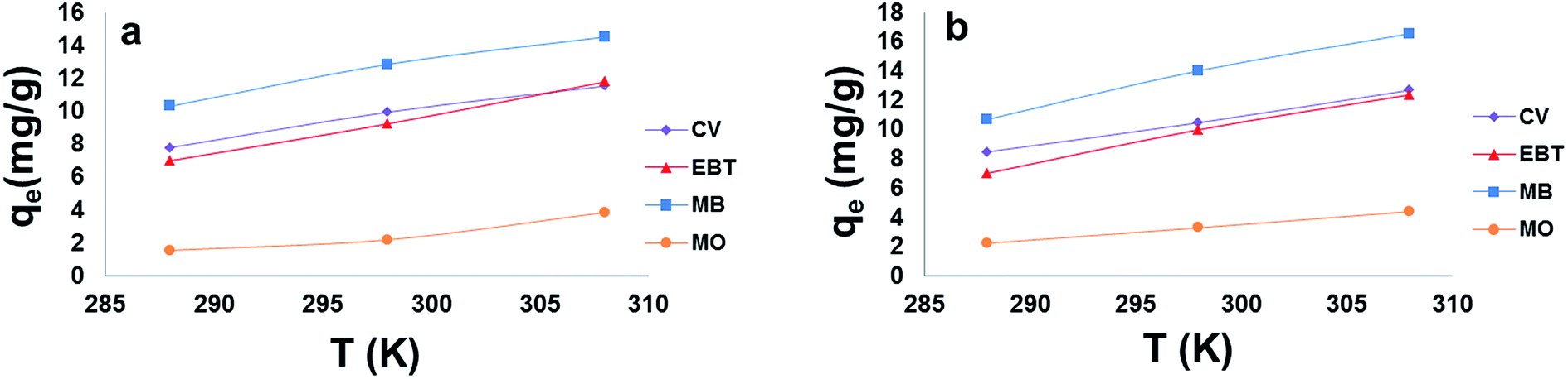 | ||
| Fig. 10 Effect of temperature on the adsorption capacity (qe) of model dyes onto; [a] MSP NPs and [b] MP NPs. Adsorbent: 5 g L−1, dyes 10 mg L−1, pH: 2.0 for anionic dyes and 8.0 for cationic dyes, time: 120 min. Magnetite/Pectin Nanoparticles: MP NPs and Magnetite/Silica/Pectin Nanoparticles: MSP NPs. | ||
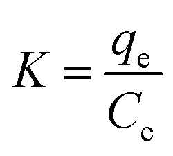
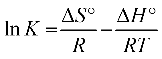
The enthalpy (ΔH°) and entropy (ΔS°) of adsorption were estimated from the slope and intercept of the plot of lnK versus 1/T yields, respectively.
The ΔH° and ΔS° values are presented in Table 9. The values are within the range of 1 to 83 kJ mol−1 and indicate the favorability of physisorption.93 The positive values of ΔH° show the endothermic nature of adsorption and also indicate the possibility of physical adsorption.93–97 The negative values of ΔG° (Table 9) show that adsorption is highly favorable for MB, CV and EBT dyes while MO showed positive values of ΔG°. Such result indicates that the MB, CV and EBT dyes adsorption was spontaneous. The positive values of ΔS° (Table 9) show the increased disorder and randomness at the solid solution interface during the adsorption of dyes on the adsorbents.67
| T (K) | K0 | ΔG° (kJ mol−1) | ΔH° (kJ mol−1) | ΔS° (J mol−1 K) | R2 | |
|---|---|---|---|---|---|---|
| MSP NPs | ||||||
| CV | 288 | 1.4426 | −0.9113 | 30.034 | 107.45 | 0.9961 |
| 298 | 2.2956 | −1.9858 | ||||
| 308 | 3.2542 | −3.06 | ||||
| MB | 288 | 3.0655 | −2.621 | 48.788 | 178.751 | 0.9999 |
| 298 | 6.1435 | −4.4796 | ||||
| 308 | 11.5079 | −6.2671 | ||||
| EBT | 288 | 0.8904 | 0.2978 | 32.747 | 112.671 | 0.9989 |
| 298 | 1.3735 | −0.8289 | ||||
| 308 | 2.1654 | −1.9556 | ||||
| MO | 288 | 0.1655 | 6.0877 | 38.298 | 111.84 | 0.9700 |
| 298 | 0.2423 | 4.9693 | ||||
| 308 | 0.4695 | 3.8509 | ||||
|
||||||
| MP NPs | ||||||
| CV | 288 | 1.4405 | −0.8412 | 31.429 | 112.048 | 0.9965 |
| 298 | 2.1434 | −1.9617 | ||||
| 308 | 3.8133 | −3.0821 | ||||
| MB | 288 | 1.9651 | −1.6249 | 44.477 | 160.078 | 0.9999 |
| 298 | 3.6966 | −3.2257 | ||||
| 308 | 6.5635 | −4.8265 | ||||
| EBT | 288 | 0.9589 | 0.0611 | 37.824 | 131.12 | 0.9968 |
| 298 | 1.7118 | −1.2501 | ||||
| 308 | 2.6717 | −2.5613 | ||||
| MO | 288 | 0.2528 | 3.2692 | 29.771 | 92.019 | 0.998 |
| 298 | 0.3957 | 2.2349 | ||||
| 308 | 0.5665 | 1.4288 | ||||
Enhancement of adsorption capacity of MSP NPs and MPs NPs at higher temperatures may be attributed to the increase in the mobility of the large dye ion with temperature. An increasing number of molecules may also acquire sufficient energy to undergo an interaction with active sites at the surface.92
3.4. Desorption and regeneration studies
The magnetite/pectin NPs and magnetite/silica pectin NPs have good performance in recycling treatment with cationic dyes. Our adsorbents did not significantly adsorb cationic dyes at pH < 3.0 (Fig. 8), which suggests that the adsorbed cationic dyes may be desorbed in solution with such pH values.98 In addition, organic cationic dyes dissolved easily in organic solvents. Thus, desorption of the cationic methylene blue dye was demonstrated with 50 mL mixture of 5% (v/v) acetic acid and methanol,71 for which about 90.0% of desorption efficiency was achieved. The results of adsorption efficiency of the studied adsorbents after three cycles are shown in Fig. 11[a]. The efficiency of adsorption decreased to two thirds after the 1st cycle and remained nearly constant throughout the 2nd and 3rd cycle for both types of adsorbents.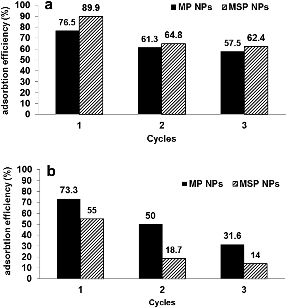 | ||
| Fig. 11 Performance of magnetite/pectin NPs (MP NPs) and magnetite/silica/pectin NPs (MSP NPs) by three cycles of adsorption/desorption for [a] methylene blue and [b] Eriochrome black T. | ||
Desorption–adsorption experiments have also been performed to evaluate the possibility of regeneration and reuse of the adsorbents for removal of anionic dyes (EBT was taken as an example). As the results show in Fig. 11[b], adsorption efficiencies were decreased by 25% from that achieved in the 1st cycle and 20% from that of the 2nd cycle. Nearly same results were obtained when using methanol alone and mixture of 5% (v/v) NaOH and methanol for EBT regeneration which elucidates that the reusability of the sorbents was better in removal of cationic dyes than in the case of anionic dyes.
3.5. Dye mixture adsorption studies
The selectivity of MP NPs and MSP NPs towards cationic and anionic dyes was investigated with initial dyes' concentration fixed at 165 mg L−1 for each dye and 2 g L−1 adsorbents mass. In former single dye adsorption studies, pH showed significant effect on the efficiency of adsorption of cationic and anionic dyes onto MP and MSP NPs. Thus the effect of pH in the range 2–8 on the removal of the model dyes mixtures (MB, CV, EBT and MO) was studied.As Fig. 12[a] and [b] show, the results agree with those obtained in the previous single dye adsorption experiments measured spectrophotometrically. For the cationic dyes (MB and CV) the adsorption was remarkably decreased in pH 2.0. The capacity of dye adsorption for MB and CV increased with increasing the solution pH from 2.0 to 8.0, reaching its maximum at 8. For the anionic dyes (MO and EBT), as observed in Fig. 12[a] and [b], the adsorption is high in acidic medium and decreases with the increase in solution pH.
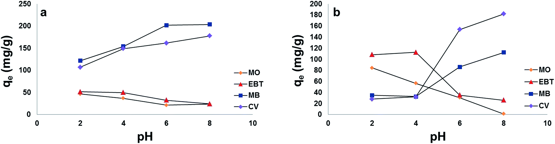 | ||
| Fig. 12 Effect of pH on the adsorption capacity (qe) of model dyes in their mixture solutions onto; [a] MSP NPs and [b] MP NPs. Adsorbent: 2 g L−1, dyes 165 mg L−1, temperature: 25 °C, time: 120 min. Magnetite/Pectin Nanoparticles: MP NPs and Magnetite/Silica/Pectin Nanoparticles: MSP NPs. | ||
Moreover, higher adsorption capacities (qe) of cationic dyes on MSP NPs (MB = 203.4 mg g−1 and CV = 177.5 mg g−1) were observed than that on MP NPs (MB = 112.2 mg g−1 and CV = 181.8 mg g−1). This also comes in agreement with the results obtained from the single dyes adsorption experiments. On the other hand, since the MP NPs offers a lesser negatively charged surface than MSP NPs in acidic pH, it favors the adsorption of anionic dyes (qe of MO = 84.4 mg g−1 and qe of EBT = 108.3 mg g−1) than that of MSP NPs (qe of MO = 46.5 mg g−1 and qe of EBT = 51.5 mg g−1).
Simultaneous adsorption of the model dyes onto MSP NPs and MP NPs was tested at natural pH of samples (pH ≈ 6) without pH adjustment as a trial for large scale wastewater treatment application. MSP NPs and MP NPs showed more adsorption towards cationic dyes (qe ranging between 86 and 201 mg g−1) than the anionic ones (qe ranging between 21 and 35 mg g−1). Such findings can be attributed to the negatively charged surface of the NPs at elevated pHs that attracts the positively charged dye molecules. Thus our proposed NPs can be applied for wastewater treatment and the removal of cationic dyes at natural pH of water samples.
4. Conclusion
In this study, we compared the physical and chemical properties of pectin coated magnetite nanoparticles prepared via two different co-precipitation techniques using data obtained by TEM, XRD, FTIR, VSM and zeta potential. Both coated NPs showed alteration in shape and particle size as indicated by TEM images which means we can have a control over the size of particles via pectin coating. FTIR spectra elucidated the successful pectin coating on magnetite and magnetite/silica NPs surfaces via carboxylate linkage. The pure magnetite phase formation was indicated by XRD data of MP NPs but upon increasing pectin concentration up to 1 w/v% other phases appeared. On the other hand, the double shell MSP NPs kept the pure magnetite phase in all prepared samples which indicated that the coating didn't affect the crystal structure of the nanoparticles. The VSM data of the MSP NPs also elucidated a minor decrease in the Ms of coated samples in comparison to the uncoated ones which indicates that the silica/pectin coating didn't cause much alteration in the NPs' magnetic properties. Yet, a great decrease in the saturation magnetization of MP NPs was observed with increasing pectin concentration. Moreover, MSP NPs had better dispersion properties than the MP NPs where the latter formed some aggregates especially in the high pectin concentration samples.The adsorption potential of MP NPs and MSP NPs was investigated for the removal of cationic and anionic dyes from aqueous systems. The effects of contact time, initial dye concentrations, pH and adsorbent mass on the adsorption process and desorption were discussed. Analysis was done using validated spectrophotometric and chromatographic methods. Adsorption kinetics was fitted with the pseudo-second-order model, and adsorption isotherms were described by Langmuir, Freundlich, Redlich–Peterson and Sips equation. The adsorption mechanism of the model dyes onto the proposed adsorbents was based on electrostatic force of attraction between cationic and anionic dyes and the adsorbents upon adjustment of pH. Regeneration of MP NPs and MSP NPs by methanol was done in order to reuse them for successive removal processes with high removal efficiency.
Simultaneous adsorption of the cationic and anionic dyes onto MSP NPs and MP NPs from dye mixture solution was tested as a trial for large scale wastewater treatment application. Higher adsorption capacities of cationic dyes on MSP NPs were observed while MP NPs favored the adsorption of anionic dyes.
In conclusion, MSP NPs and MP NPs are promising alternatives for cationic and anionic dyes removal from wastewater because of their high adsorption capacities and separation convenience. We believe that the approach presented herein can provide a convenient way to bind other cationic and anionic organic compound or heavy metal ions to our magnetic absorbents and to quickly separate them from wastewater.
Acknowledgements
This research was supported by science and technology development fund (STDF), Egypt. Project number 12641.References
- L. Ai, C. Zhang, F. Liao, Y. Wang and M. Li, J. Hazard. Mater., 2011, 198, 282–290 CrossRef CAS PubMed.
- O. Legrini, E. Oliveros and A. Braun, Chem. Rev., 1993, 93, 671–698 CrossRef CAS.
- S. Li, Bioresour. Technol., 2010, 101, 2197–2202 CrossRef CAS PubMed.
- N. Bao, Y. Li, Z. Wei, G. Yin and J. Niu, J. Phys. Chem. C, 2011, 115, 5708–5719 CAS.
- B. Inbaraj and B. Chen, Bioresour. Technol., 2011, 102, 8868–8876 CrossRef PubMed.
- R. Rakhshaee and M. Panahandeh, J. Hazard. Mater., 2011, 189, 158–166 CrossRef CAS PubMed.
- P. S. Guru and S. Dash, J. Dispersion Sci. Technol., 2012, 33, 1012–1020 CrossRef CAS.
- S. Oh, D. Cha, P. Chiu and B. Kim, Water Sci. Technol., 2004, 49, 129–136 CAS.
- J. Perey, P. Chiu, C. Huang and D. Cha, Water Environ. Res., 2002, 74, 221–225 CrossRef CAS PubMed.
- A. Afkhami and R. Moosavi, J. Hazard. Mater., 2010, 174, 398–403 CrossRef CAS PubMed.
- C. Yavuz, J. Mayo, W. William and A. Prakash, Science, 2006, 314, 964–967 CrossRef PubMed.
- A. Afkhami, M. Saber-Tehrani and H. Bagheri, Desalination, 2010, 263, 240–248 CrossRef CAS.
- A. Gupta and M. Gupta, Biomaterials, 2005, 26, 3995–4021 CrossRef CAS PubMed.
- S. Mak and D. Chen, Dyes Pigm., 2004, 61, 93–98 CrossRef CAS.
- S. Huang and D. Chen, J. Hazard. Mater., 2009, 163, 174–179 CrossRef CAS PubMed.
- S. Banerjee and D. Chen, J. Hazard. Mater., 2007, 147, 792–799 CrossRef CAS PubMed.
- C. Vilhena, M. Goncalves and A. Mota, Electroanalysis, 2004, 16, 2065–2072 CrossRef CAS.
- GITCO, 1999.
- A. Konno, M. Miyawaki, M. Misaki and K. Yasumatsu, Agric. Biol. Chem., 2014, 45, 2341–2342 CrossRef.
- A. Madhav, M.Sc. thesis, Kerala Agricultural University, Thrissur, 2001, p. 52.
- A. Cucheval, M. A. Al-Ghobashy, Y. Hemar, D. Otter and M. A. K. Williams, J. Colloid Interface Sci., 2009, 338, 450–462 CrossRef CAS PubMed.
- A. A. S. Raj and T. V. Ranganathan, Sci. Rep., 2012, 1, 553, DOI:10.4172/scientificreports.553.
- Y. Lin, C. Weng and F. Chen, Sep. Purif. Technol., 2008, 64, 26–30 CrossRef CAS.
- F.-T. J. Ngenefeme, N. J. Eko, Y. D. Mbom, N. D. Tantoh and K. W. M. Rui, Open J. Compos. Mater., 2013, 03, 30–37 CrossRef CAS.
- http://www.wiredchemist.com/chemistry/data/acid-base-indicators, accessed at October 12, 2015.
- http://www.chemicalbook.com/, accessed at October 12, 2015.
- http://pubchem.ncbi.nlm.nih.gov/, accessed at October 12, 2015.
- http://en.wikipedia.org/wiki/, accessed at October 12, 2015.
- International Conference on Harmonization (ICH), Q2B, Validation of Analytical Procedures, US FDA Federal Register, 1994, accessed at October 12, 2015 Search PubMed.
- International Conference on Harmonization (ICH), Q2, Validation of Analytical Procedures, 2005 Search PubMed.
- International Conference on Harmonization (ICH), Q2B, Validation of Analytical Procedures: Definitions and Terminology, US FDA Federal Register, 1995, vol. 60 Search PubMed.
- J.-L. Gong, X.-Y. Wang, G.-M. Zeng, L. Chen, J.-H. Deng, X.-R. Zhang and Q.-Y. Niu, Chem. Eng. J., 2012, 185–186, 100–107 CrossRef CAS.
- Z. Lei, X. Pang, N. Li, L. Lin and Y. Li, J. Mater. Process. Technol., 2009, 209, 3218–3225 CrossRef CAS.
- M. Seenuvasan, C. G. Malar, S. Preethi, N. Balaji, J. Iyyappan, M. A. Kumar and K. S. Kumar, Mater. Sci. Eng., C, 2013, 33, 2273–2279 CrossRef CAS PubMed.
- Markandeya, S. P. Shukla and G. C. Kisku, Res. J. Environ. Toxicol., 2015, 9, 320–331 CrossRef.
- D. Confortin, H. Neevel, M. Brustolon, L. Franco, A. J. Kettelarij, R. M. Williams and M. R. van Bommel, J. Phys.: Conf. Ser., 2010, 231, 012011 CrossRef.
- U. The United States Pharmacopoeia & National Formulary, US Pharmacopoeial Convention Inc., 2011.
- W. H. Organization, The International Pharmacopoeia, World Health Organization, 2006, vol. 1 Search PubMed.
- A. Bee, R. Massart and S. Neveu, J. Magn. Magn. Mater., 1995, 149, 6–9 CrossRef CAS.
- S. Liang, X. Guo, N. Feng and Q. Tian, J. Hazard. Mater., 2010, 174, 756–762 CrossRef CAS PubMed.
- T. T. Baby and S. Ramaprabhu, Talanta, 2010, 80, 2016–2022 CrossRef CAS PubMed.
- J. Liu, Z. Zhao and G. Jiang, Environ. Sci. Technol., 2008, 42, 6949–6954 CrossRef CAS PubMed.
- D. Predoi, R. Clerac, A. Jitianu, M. Zaharescu, M. Crisan and M. Raileanu, Digest Journal of Nanomaterials and Biostructures, 2006, 1, 93–97 Search PubMed.
- E. V. Escobar Zapata, C. A. Martínez Pérez, C. A. Rodríguez González, J. S. Castro Carmona, M. A. Quevedo Lopez and P. E. García-Casillas, J. Alloys Compd., 2012, 536, S441–S444 CrossRef CAS.
- A. L. Andrade, D. M. Souza, M. C. Pereira, J. D. Fabris and R. Z. Domingues, Ceramica, 2009, 55, 420–424 CAS.
- M. Mikhaylova, D. K. Kim, N. Bobrysheva, M. Osmolowsky, V. Semenov, T. Tsakalakos and M. Muhammed, Langmuir, 2004, 20, 2472–2477 CrossRef CAS PubMed.
- Z. Ma, Y. Guan and H. Liu, J. Polym. Sci., Part A: Polym. Chem., 2005, 43, 3433–3439 CrossRef CAS.
- R. K. Dutta and S. Sahu, Eur. J. Pharm. Biopharm., 2012, 82, 58–65 CrossRef CAS PubMed.
- S. Theerdhala, D. Bahadur, S. Vitta, N. Perkas, Z. Zhong and A. Gedanken, Ultrason. Sonochem., 2010, 17, 730–737 CrossRef CAS PubMed.
- R. M. Cornell and V. Schwertmann, The Iron Oxides: Structure, Properties, Reactions, Occurrence and Uses, VCH Publishers, Weinheim, 2nd edn, 2003 Search PubMed.
- S. K. Giri, N. N. Das and G. C. Pradhan, Colloids Surf., A, 2011, 389, 43–49 CrossRef CAS.
- M. Szekeres, I. Y. Tóth, E. Illés, A. Hajdú, I. Zupkó, K. Farkas, G. Oszlánczi, L. Tiszlavicz and E. Tombácz, Int. J. Mol. Sci., 2013, 14, 14550–14574 CrossRef PubMed.
- R. H. Müller and G. E. Hildebrand, J. Drug Targeting, 1996, 4, 161–170 CrossRef PubMed.
- A. Debrassi, A. F. Corrêa, T. Baccarin, N. Nedelko, A. Ślawska-Waniewska, K. Sobczak, P. Dłużewski, J.-M. Greneche and C. A. Rodrigues, Chem. Eng. J., 2012, 183, 284–293 CrossRef CAS.
- R. D. Ambashta and M. Sillanpää, J. Hazard. Mater., 2010, 180, 38–49 CrossRef CAS PubMed.
- S. Chatterjee, D. S. Lee, M. W. Lee and S. H. Woo, Bioresour. Technol., 2009, 100, 2803–2809 CrossRef CAS PubMed.
- A. M. Etorki and F. M. Massoudi, Orient. J. Chem., 2011, 27, 875–884 CAS.
- N. Saad, M. Al-Mawla, E. Moubarak, M. Al-Ghoul and H. El-Rassy, RSC Adv., 2015, 5, 6111–6122 RSC.
- I. Langmuir, J. Am. Chem. Soc., 1918, 40, 1361–1403 CrossRef CAS.
- H. Freundlich, Über die Adsorption in Lösungen, Engelmann, 1906 Search PubMed.
- O. Redlich and D. L. Peterson, J. Phys. Chem., 1959, 63, 1024 CrossRef CAS.
- R. Sips, J. Chem. Phys., 1948, 16, 490 CrossRef CAS.
- A. Z. M. Badruddoza, G. S. S. Hazel, K. Hidajat and M. S. Uddin, Colloids Surf., A, 2010, 367, 85–95 CrossRef CAS.
- R. Sivashankar, A. B. Sathya, K. Vasantharaj and V. Sivasubramanian, Environmental Nanotechnology, Monitoring & Management, 2014, 1–2, 36–49 Search PubMed.
- F.-C. Wu, B.-L. Liu, K.-T. Wu and R.-L. Tseng, Chem. Eng. J., 2010, 162, 21–27 CrossRef CAS.
- S. G. Muntean, O. Paska, S. Coseri, G. M. Simu, M. E. Grad and G. Ilia, J. Appl. Polym. Sci., 2013, 127, 4409–4421 CrossRef CAS.
- O. M. Paşka, C. Păcurariu and S. G. Muntean, RSC Adv., 2014, 4, 62621–62630 RSC.
- L. B. L. Lim, N. Priyantha and N. H. M. Mansor, Environ. Earth Sci., 2014, 73, 3239–3247 CrossRef.
- T. S. Anirudhan, P. G. Radhakrishnan and K. Vijayan, Sep. Sci. Technol., 2013, 48, 947–959 CrossRef CAS.
- E. Bulut, M. Özacar and İ. Şengil, J. Hazard. Mater., 2008, 154, 613–622 CrossRef CAS PubMed.
- F. Ge, H. Ye, M.-M. Li and B.-X. Zhao, Chem. Eng. J., 2012, 198–199, 11–17 CrossRef CAS.
- T. Madrakian and A. Afkhami, J. Hazard. Mater., 2011, 196, 109–114 CrossRef CAS PubMed.
- K. Singh, S. Gupta, A. Singh and S. Sinha, J. Hazard. Mater., 2011, 186, 1462–1473 CrossRef CAS PubMed.
- M. Gabal and E. Al-Harthy, Chem. Eng. J., 2014, 255, 156–164 CrossRef CAS.
- T. Madrakian, A. Afkhami and M. Ahmadi, Spectrochim. Acta, Part A, 2012, 99, 102–109 CrossRef CAS PubMed.
- L. Ai, C. Zhang and Z. Chen, J. Hazard. Mater., 2011, 192, 1515–1524 CrossRef CAS PubMed.
- L. Cottet, C. Almeida and N. Naidek, Appl. Clay Sci., 2014, 95, 25–31 CrossRef CAS.
- P. Dave, S. Kaur and E. Khosla, Indian J. Chem. Technol., 2011, 18, 53–60 CAS.
- N. Barka, M. Abdennouri and M. Makhfouk, J. Taiwan Inst. Chem. Eng., 2011, 42, 320–326 CrossRef CAS.
- F. Moeinpour, A. Alimoradi and M. Kazemi, J. Environ. Health Sci. Eng., 2014, 12, 112 CrossRef PubMed.
- O. Elijah and N. T. Joseph, SOP Transactions on Applied Chemistry, 2014, 1, 14–25 CrossRef.
- J. Pal, M. K. Deb, D. K. Deshmukh and D. Verma, Appl. Water Sci., 2013, 3, 367–374 CrossRef CAS.
- E. Bazrafshan, A. Zarei, H. Nadi and M. Zazouli, Indian J. Chem. Technol., 2014, 21, 105–113 CAS.
- Z. Haddadian and M. Shavandi, Chem. Sci. Trans., 2013, 2, 900–910 CAS.
- C. Umpuch and S. Sakaew, Songklanakarin J. Sci. Technol., 2013, 35, 451–459 CAS.
- S. Koner, B. Saha, R. Kumar and A. Adak, Int. J. Curr. Res., 2011, 3, 128–133 Search PubMed.
- R. Jiang, Y. Fu and H. Zhu, J. Appl. Polym. Sci., 2012, 125, E540–E549 CrossRef CAS.
- L. Wang, J. Li, Y. Wang and L. Zhao, J. Hazard. Mater., 2011, 196, 342–349 CAS.
- S. Lagergren, About the theory of so-called adsorption of soluble substances, Kungliga Svenska Vetenskapsakademiens, Handlingar 24, 1898 Search PubMed.
- Y. Ho and G. McKay, Process Biochem., 1999, 34, 451–465 CrossRef CAS.
- G. Vijayakumar, R. Tamilarasan and M. Dharmendirakumar, J. Mater. Environ. Sci., 2012, 3, 157–170 CAS.
- M. Doğan, M. Alkan and Y. Onganer, Water, Air, Soil Pollut., 2000, 120, 229–248 CrossRef.
- M. Hema and S. Arivoli, J. Appl. Sci. Environ. Manage., 2008, 12, 43–51 Search PubMed.
- H. Xu, Y. Xu and Y. Chen, Adv. Mater. Res., 2011, 194–196, 488–491 CAS.
- M. Arshadi, F. SalimiVahid, J. W. L. Salvacion and M. Soleymanzadeh, RSC Adv., 2014, 4, 16005 RSC.
- J. X. Zhang and L. L. Ou, Water Sci. Technol., 2013, 67, 737–744 CrossRef CAS PubMed.
- S. Hong, C. Wen, J. He, F. Gan and Y.-S. Ho, J. Hazard. Mater., 2009, 167, 630–633 CrossRef CAS PubMed.
- Y. Lin, H. Chen and P. Chien, J. Hazard. Mater., 2011, 185, 1124–1130 CrossRef CAS PubMed.
Footnote |
| † Electronic supplementary information (ESI) available. See DOI: 10.1039/c5ra23452b |
| This journal is © The Royal Society of Chemistry 2016 |