Topological analysis of non-granular, disordered porous media: determination of pore connectivity, pore coordination, and geometric tortuosity in physically reconstructed silica monoliths

Abstract

Gaining adequate knowledge on the morphology of porous media is critical to ensuring their continued success as support structures in applications that rely on efficient mass transport. The physical reconstruction of a porous medium provides the optimum basis for an accurate characterization of its morphology, yet the identification of meaningful descriptors is not straightforward, especially not for monolithic materials, whose continuous solid phase and open pore network resist the tessellation schemes applicable to granular media. In this work, we focus on a hardly investigated component of silica monolith morphology, namely the topology of the hydrodynamically accessible macropore space. We propose and apply suitable methods to determine pore connectivity, pore coordination, and geometric tortuosity in four silica monolith samples after physical reconstruction of their macropore space by confocal laser scanning microscopy. Pore connectivity is traced by medial axis analysis, whereas pore coordination is evaluated after compartmentalization of the open macropore space into individual pores and pore throats by a maximum inscribed spheres approach. The geometric tortuosity is determined by medial axis analysis as well as by a propagation method that maps the geodesic distance from the center point of a reconstruction to every other point in the pore space. The presented results provide a comprehensive description of silica monolith topology as well as quantitative data for the construction of pore network models. The proposed analysis methods are applicable to any porous material that can be physically reconstructed at the required resolution.

---

1 Introduction

Silica-based materials with a hierarchical pore space are of substantial technical relevance as support structures for chemical separations^1–3 and heterogeneous catalysis.^4–6 In silica monoliths, a hierarchical pore space architecture is realized through a continuous silica skeleton perforated by intersecting networks of larger and smaller pores.^7–10 Macropores (>50 nm) provide fast, advection-dominated mass transport through the material; micro- and mesopores (<2 nm and 2–50 nm, respectively), which are accessible only by diffusion, generate a large surface area for adsorption and reaction of solutes. Silica monoliths are prepared in a polycondensation reaction. Macropores and a microporous silica skeleton are formed during the sol–gel transition that accompanies spinodal decomposition of the reactants.⁷ In a second step, the micropores in the silica skeleton are widened into mesopores, for example, through thermal treatment. The mesopore space can also be generated by alternative routes, for example, by transforming the silica skeleton into an MCM-41-type pore structure (i.e., an ordered structure) under conditions that preserve the original morphology and macroporosity of the material.¹¹ The successive preparation of macro- and mesopore space enables an independent adjustment of permeability, surface area, and textural characteristics, which gives the materials chemist in principle a much wider influence over the properties of the final product than possible with traditional particulate packings (packed beds), whose permeability is dependent on the particle size and is limited by the requirement of mechanical stability under high pressure.

High-performance liquid chromatography (HPLC) is not only an important application of particulate packings and monoliths as separation columns, but also a valuable and easily available method to probe the complex relationship between the morphology and the mass transport properties of the employed porous medium. In HPLC, the separation efficiency is mainly determined by the uniformity of the pressure-driven flow field in the macropore space as well as by the resistance to mass transfer between macropores and mesopores.^12,13 The first generation of silica monoliths prepared for use as analytical HPLC columns suffered from large average macropore sizes, wide macropore size distributions, as well as from variations in porosity and macropore size over the column cross-section.^1,14,15 In recent years the preparation process has been substantially improved,^16–20 culminating in the so-called second generation of silica monoliths.²¹ With negligible radial heterogeneity and macropores reaching the sub-μm regime,²² second-generation monoliths demonstrate higher separation efficiencies.^15,22,23 Remarkably, in addition to their radially homogeneous macropore and skeleton size distributions,¹⁵ the second-generation monoliths realize smaller macropore sizes at even increased macropore homogeneity with respect to the first-generation monoliths.^15,22

Apart from characterizing the morphology of silica monoliths according to their performance as HPLC columns, morphological information is available from various other indirect methods. Most prominent among them are mercury intrusion porosimetry for the macropores and nitrogen physisorption for the micro- and mesopores.^24–27 These methods are fast and convenient, but provide no local resolution. The generated data are converted into pore size distributions by assuming a certain morphology, that is, a specific pore shape and connectivity. The current morphological models have been recognized as too simplistic, but the development of better models awaits the availability of accurate morphological information.

The obvious solution to the problem are direct methods that reveal the true morphology of silica monoliths. Several methods are able to provide a spatially resolved picture of the macropore space, whereas the much smaller mesopores can be resolved only with transmission electron microscopes and micropores have not been imaged yet. Basic imaging methods like scanning electron microscopy (SEM) lack depth information and thus cannot provide a faithful three-dimensional (3D) image of the macropore space. The latter requires imaging techniques with tomographic capabilities, such as focused ion beam (FIB)-SEM, serial block face (SBF)-SEM, and confocal laser scanning microscopy (CLSM).^28–39 Combined with advanced image processing methods, the acquired data enable to physically reconstruct the exact structure of a material. CLSM and FIB-SEM have both successfully been used to reconstruct the macropore space of silica-based structures.^37,40–43 Our group has focused on the reconstruction of particulate packings and silica monoliths in capillary and analytical column format.^{15,22,44–46} The geometrical properties of the macropore space, that is, how the void space is distributed over the column, were accurately derived by statistical analysis methods. Combined with numerical simulations,^47–50 the collected morphological data allowed us to evaluate the flow, diffusion, and dispersion properties of a material, to calculate its theoretical separation efficiency as a chromatographic column, and to find out why a further reduction of macropore size in second-generation silica monoliths did not result in the expected gain in separation efficiency.^22,43,51,52

Compared with the geometrical aspect of macropore space morphology, the topological aspect, that is, how the pores are coordinated and connected as well as how tortuous (sinuous) the pathways through the pore space are, has received little attention so far. In the current work, we attempt a comprehensive analysis of the macropore space topology by using complementary approaches to gather data on pore interconnection and geometric tortuosity. As representative samples we selected commercially available silica monoliths intended for use as analytical HPLC columns. Importantly, these samples are employed here merely to help us illustrating general methodology and the application of accompanying software. It will guide the materials scientist in analyzing the topological properties of a material at hand in all relevant detail and especially in comparing materials obtained with distinct modifications of their synthesis. We reconstruct the macropore space of each monolith by CLSM and determine the most relevant geometrical properties, namely average macropore size and skeleton thickness, by chord length distribution (CLD) analysis.^15,22 The first step of the topological analysis relies on skeletonization of the pore space.^{37,43,53–56} A thinning algorithm reduces the pore space to a continuous medial axis, from which values for the pore connectivity and geometric tortuosity are derived. The determination of pore connectivity and geometric tortuosity by medial axis analysis (MAA) does not require to define the limits of individual pores, similar to how CLD analysis yields the geometrical properties of the macropore space without defining (and assigning a size to) individual pores. In contrast, the second step of the topological analysis relies on compartmentalization of the pore space. We use a maximum inscribed spheres approach (MISA) to divide the open macropore space of a silica monolith into a set of individual pores.^57–61 MISA supplements the solid–void borders present in the silica monolith with calculated void–void borders that delimit individual pores from each other. The calculated borders are located along local minima of solid–void distances and in this way resemble pore throats that connect larger voids with each other. The compartmentalized version of the macropore space allows to determine the number of pores a given pore shares pore throats with (the pore coordination) as well as the number of pores that share a given pore throat (the pore throat coordination). These data provide the link to pore network models, which, by reducing the complexity of a pore space into a simpler network of pores and pore throats, enable simulations of multiphase flow, wettability, or precipitation^60,62–64 as well as the interpretation of porosimetry and physisorption data. The third step of the topological analysis works directly with the reconstructed macropore space. By mapping the geodesic distances between the center point and all other points in the void space of a reconstructed sample, we determine the global geometric tortuosity of the macropore space.

The primary goal of this study is to complement our knowledge about the macropore space geometry of silica monoliths with quantitative data on the topology. Further, we want to propose and share suitable methods for the topological analysis of disordered porous media, particularly (but not exclusively) monolithic materials.

2 Materials and methods

2.1 Chemicals and materials

Laboratory samples of silica monoliths prepared according to an established procedure¹⁸ were generously given by Merck Millipore (Darmstadt, Germany) as cylindrical bare-silica rods of 4.6 mm I.D. × 150 mm length. Samples #1, #2, and #3 are second-generation monoliths (from different preparation charges), sample #4 is a first-generation monolith. This set of monoliths thus addresses timely, representative samples, which here serve exclusively to illustrate the general methodology for topological analysis. The fluorescent dye Bodipy 493/503 was bought from Life Technologies (Darmstadt, Germany). Dimethyl sulfoxide (DMSO), glycerol, and octadecyltrimethoxysilane as well as HLPC-grade acetone, ethanol, and toluene were from Sigma Aldrich Chemie (Taufkirchen, Germany). HPLC-grade water was obtained from a Milli-Q gradient water purification system (Millipore, Bedford, MA).

2.2 Confocal laser scanning microscopy

2.2.1 Sample preparation. Cylindrical disks (ca. 1 mm thick) were cut at about mid-length from the bare-silica rods using a water-cooled circular saw. Cuts were made orthogonal to the cylinder axis. The disks were washed with ethanol and toluene, and then immersed in an octadecyltrimethoxysilane solution (220 mg mL⁻¹ in toluene) for 6 h at 343 K. The disks were then washed with toluene and acetone before being immersed in a Bodipy 493/503 solution (0.5 mg mL⁻¹ in acetone) for 12 h. The pore space was filled 1 h before the microscopic investigation with a glycerol/DMSO/water mixture (70/19/11, v/v/v) to match the optical dispersion behavior of monolithic silica.^44,45 Prior to use the refractive index at the sodium D line (n_D = 1.4582) of the matching liquid was verified using a digital refractometer (Reichert Analytical Instruments, Depew, NY).

2.2.2 Image acquisition. Microscopic experiments were performed on a TCS SP5 II confocal microscopy system equipped with a HCX PL APO 63x/1.3 GLYC CORR CS (21°) glycerol immersion objective lens (Leica Microsystems, Wetzlar, Germany). A custom-made sample holder was used to mount the silica disks directly beneath a ‘type 0’ cover slip (Gerhard Menzel GmbH, Braunschweig, Germany). The refractive index matching liquid was used as immersion and embedding liquid to minimize spherical aberrations.⁴⁵ The Bodipy dye was excited at a wavelength of 488 nm. Emitted light was detected at the interval of 491–515 nm. The sampling step size was adjusted to 30 nm in lateral direction and to 126 nm in axial direction to comply with the Nyquist criterion.

Stacks of 150–200 grayscale images (8-bit, 2048 × 2048 pixels) were acquired at arbitrarily chosen locations on the disk, but at a distance of at least 10 μm from the disk surface to avoid imaging morphological distortions generated by the cutting process. The propagation direction z of the image-stack acquisition was perpendicular to the disk surface, that is, parallel to the axis of the cylindrical column from which the disk had been cut.

2.2.3 Image processing. Microscopic images were restored and segmented in a four-step procedure: (1) photon noise was reduced using the PureDenoise ImageJ plug-in.⁶⁵ (2) Photobleaching was corrected with an intensity adjustment based on fitting an exponential decay function to the z-axis of the image stack. (3) Huygens maximum likelihood iterative deconvolution (Scientific Volume Imaging, Hilversum, The Netherlands) was applied. (4) Segmentation was carried out by subtraction of a Gaussian blurred image stack copy (kernel size = 200 pixels) from the initial image stack. This last step was repeated once with the image data obtained from the first segmentation. After this process, all pixels with an intensity value of zero were assigned as void (macropore) space; the remaining non-zero pixels were considered as solid phase (silica skeleton). To eliminate artifacts at the borders of the image stack, five slices were discarded from top and bottom of the stack and images were symmetrically cropped to 2000 × 2000 pixels. The final physically reconstructed volume of each investigated silica monolith was 60 μm × 60 μm × 18–25 μm.

2.3 Morphological analysis

2.3.1 Chord length distributions. The geometrical properties of the reconstructed macropore spaces were evaluated by CLDs.^66–68 A CLD was obtained by placing seed points randomly into the void space.^15,22,44,69 32 equiangular distributed vectors per seed point were spread out until they reached the solid–void border.^51,70 The length of a chord consisting of two opposing vectors was collected in a histogram, unless one vector projected out of the image bounds, in which case the chord was discarded. Histograms contained 10⁶ chords at a bin size of 0.2 μm. Using the Levenberg–Marquardt algorithm,⁷¹ histograms were fitted to the k-Gamma function: For the investigated, microscopically disordered monoliths the use of the k-Gamma function to describe their void volume fluctuations can be motivated from a statistical mechanics point of view.⁷² We have previously observed that the k-Gamma function accurately fits CLDs generated in the macropore space of physically reconstructed packed beds^45,73 and silica as well as organic–polymer monoliths.^{15,22,36,37,39,51} In eqn (1)l_c is the chord length, Γ the Gamma function, μ the first statistical moment, and k = (μ/σ)² the second statistical moment of the distribution. A CLD of the silica skeleton was obtained by generating chords in the solid phase rather than the void space. Solid phase CLDs of monolithic materials have also been found to be well described by the k-Gamma function.^15,36,39,43 The values for μ and k obtained from fitting the CLD to the k-Gamma function are quantitative measures for the average size and for the homogeneity of the size distribution of the investigated (solid or void) phase, respectively.^15,22,50,51

2.3.2 Medial axis generation. An iterative-thinning algorithm, available as an ImageJ plug-in bundle (Skeletonize3D and AnalyzeSkeleton), was applied to reduce the macropore space to a medial axis of one voxel thickness under conservation of its topological properties.^65,74,75 An average pore connectivity Z was calculated as the average number of branches of the medial axis meeting at a junction (i.e., a node of the medial axis network):withwhere n_j is the total number of junctions, n_t is the number of triple-point junctions (connecting three branches), n_q the number of quadruple-point junctions (connecting four branches), and n_x the number of higher-order junctions (connecting five or more branches). Therefore, n_t/n_j, n_q/n_j and n_x/n_j give the fraction of nodes in the network connecting 3, 4 or >4 branches, respectively.

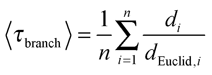
The average value of the geometric branch tortuosity 〈τ_branch〉 was calculated as the average of all node-to-node network distances d_i over the Euclidean distances d_Euclid,i between these nodes:

2.3.3 Sphere inscription. The reconstructed macropore space of a silica monolith was compartmentalized by a four-step algorithm developed by us building on previous work by Dong and Blunt.⁵⁹ We provide here a brief description; detailed information and the software download can be found elsewhere.⁷⁶ (1) Starting from the 3D binary image of solid and void voxels, a sphere that just touched the solid–void border was inscribed around each void voxel by determining the smallest distance between the particular void voxel and the solid phase through Euclidean distance transform.^77–81 In the resulting Euclidean distance transform field, each void voxel was assigned the radius of its surrounding maximum inscribed sphere. The field contained as many maximum spheres as the binary image contains void voxels. (2) The large set of maximum inscribed spheres meant that a particular void voxel could be part of (covered by) several spheres. The set of maximum spheres was reduced to a subset of containing spheres by searching for each void voxel for the largest sphere in which this voxel was contained and assigning the containing sphere radius to the voxel. This implies that spheres contained within a larger sphere as well as spheres contained by a union of two or more larger spheres were eliminated. After completion of step 2, all void voxels were unequivocally assigned the radius of their largest containing sphere. (3) Either single containing spheres or unions of containing spheres with equal radii formed local maxima (plateaus) in the containing sphere radius (CSR) field. We used the centers of these spheres as the seed points for pore propagation. Starting from the seed voxel with the largest assigned CSR value as the first pore seed, the neighboring void voxels were assigned as belonging to the pore sprouting from the current seed for as long as their CSR values were equal to or smaller than that of their direct predecessor. Then, the pore seed with the next-to-largest CSR value was propagated, and so on. If pore propagation reached voxels that had already been assigned as belonging to another pore, these voxels were marked as shared pore voxels. After completion of this step, all void voxels in the 3D image were assigned as either belonging to a certain pore or as shared-pore voxels. (4) Finally, shared-voxel volumes were reduced to single-voxel-thick boundary layers by a variant of the watershed segmentation.^82,83 The CSR values were interpreted as the depth of the relief where watershed happens. The water level was initially set at the largest CSR value among the pore seeds (i.e., the deepest point in the relief) and then stepwise increased. At each iteration, the boundary voxels at the current water level for each pore as well as the 26 neighbors of every propagation boundary voxel were processed. If a neighbor was (i) a void voxel and (ii) its CSR value was not larger than those of the current boundary voxel, the boundary could propagate to this voxel. If the neighbor did not belong to any pore yet, we marked the neighbor as belonging to the current pore and added it to the pore boundary (to be processed on the next iteration). If the neighbor was already marked as belonging to one or more pores, we specified that the neighbor belonged to the current pore as well, did not add it to the pore boundary, and removed it from the boundaries of other pores to which it belonged (to be processed on current or future iteration steps). After processing all boundary voxels at the current water level, the water level was increased by one step and pore propagation resumed. This procedure was repeated until, after a final increase of the water level, no boundary voxels were left for pore propagation. Following watershed segmentation, all void voxels were assigned as either belonging to a certain pore or as belonging to a boundary layer between two or more pores (i.e., a pore throat). The 3D image then contained solid voxels, pore voxels, and pore-throat voxels.

2.3.4 Geodesic distance propagation. The geodesic distance d_g is the shortest path between two locations in the void space that does not cross the silica skeleton at any point. We calculated the geodesic distances between a single starting point and all other void voxels in the 3D image.⁵⁹ Starting from the void voxel closest to the geometric center of the reconstructed volume, we calculated the shortest paths to all other void voxels employing Dijkstra's shortest path algorithm.⁸⁴ Each voxel was connected to 26 neighbors, excepting solid voxels, which were excluded from the analysis. A void voxel was treated as a vertex in a graph. The Euclidean distance between voxels was used as a weight of edges in this graph and could thus take only values of 1, , or .

The global geometric tortuosity τ_geo is the ratio of d_g to d_Euclid for the case of sufficiently long geodesic distances:⁸⁵

where d_Euclid is the Euclidean distance between starting and current voxel. We used about 2.6 × 10⁶ values per reconstructed sample volume for calculating the global geometric tortuosity. More information and the software download can be found elsewhere.⁷⁶

3 Results and discussion

3.1 Geometrical characterization by chord length distribution analysis

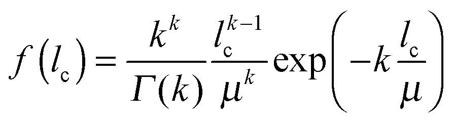
Of each investigated silica monolith, a volume of 60 μm × 60 μm × 18–25 μm was physically reconstructed for morphological analysis. As first step we characterized the average geometrical properties of the macropore space (Table 1) as reference for the subsequent topological analysis. The external porosity (ε_ext) was calculated as the fraction of void voxels in a reconstructed volume. Average macropore size (μ_macro) and average skeleton thickness (μ_skel) were determined by CLD analysis. CLD analysis allows to determine the size distribution of each phase of a porous medium without defining the geometry of three-dimensional objects. This is especially valuable for monolithic materials, where both, void space and solid phase, are continuous. Fig. 1A shows how chords were generated in the reconstructed macropore space of a silica monolith. The chord lengths were collected into a macropore CLD, which was then fitted to the k-Gamma function to determine μ_macro (Fig. 1B). μ_skel was analogously received by generating chords in the solid phase and fitting the resulting skeleton CLD to the k-Gamma function. The data in Table 1 show that the monoliths share a highly similar external porosity of 65–68%, whereas average macropore size and skeleton thickness nearly double in value from monolith #1 with μ_macro = 2.54 μm and μ_skel = 1.13 μm to monolith #4 with μ_macro = 4.93 μm and μ_skel = 2.01 μm. The microscopy images shown in Fig. 1C visualize the fine structure of monolith #1 next to the coarse structure of monolith #4, both at an external porosity of 67%. Over the investigated sample set, average macropore size and skeleton thickness increase in the same direction, maintaining a ratio of 2–2.5 (Table 1). In principle, macropore size and skeleton thickness are considered independently adjustable parameters.¹ In practice, however, when data from several silica monolith samples are surveyed (usually values for the domain size and the skeleton diameter estimated from SEM images) a constant relation between macropore size and skeleton thickness is found.^2,14,22 For monoliths intended as HPLC columns, smaller macropores may be desirable to decrease hydrodynamic dispersion in the system and thus further improve the separation efficiency. Decreasing the skeleton thickness along with the macropore size shortens the pathways for diffusion-limited mass transport, which may be desirable as well, as long as the monolith's mechanical stability is not endangered. In the following, we turn to the topological properties of the investigated silica monoliths, which will be referenced by their average macropore size (μ_macro).

Table 1 Average geometrical properties of the investigated silica monoliths. Average macropore size and skeleton thickness were determined by CLD analysis. The external porosity was determined as the fraction of void voxels within a reconstructed volume

Monolith	μ macro (μm)	μ skel (μm)	μ macro/μskel	ε ext (%)
#1	2.54	1.13	2.25	67.1
#2	3.35	1.65	2.03	64.9
#3	4.00	1.64	2.44	67.5
#4	4.93	2.01	2.45	66.6

---

Fig. 1 (A) Scheme illustrating the generation of chords in the reconstructed macropore space of a silica monolith (white – silica skeleton, black – void space). Seed points (P1 to P3, yellow) are randomly distributed over the entire void space. From every seed point vectors are spread in 32 equiangular directions. If two opposing vectors reach the solid–void border, the sum of both vector lengths is counted as a chord length (green); otherwise, the vector pair is discarded (red). Chord lengths are collected into a macropore CLD. (B) k-Gamma function fits of the macropore CLDs and the average macropore size (μ_macro) obtained for each silica monolith. (C) Binary images of monoliths #1 (left, μ_macro = 2.54 μm) and #4 (right, μ_macro = 4.93 μm) visualize a fine and a coarse structure, respectively, at the same external porosity (ε_ext ≈ 67%).

3.2 Topological characterization by medial axis analysis

We begin the topological characterization of the monoliths' macropore space by MAA, a method that acknowledges the continuous nature of the silica skeleton and the open structure of the macropore network. A thinning algorithm reduces the pore space to a medial axis of one voxel thickness, while the topological character of the pore space is conserved.⁷⁵Fig. 2 gives an impression of how the macropore space is traced by a voxel line that branches at every junction of the network to enter abducent channels.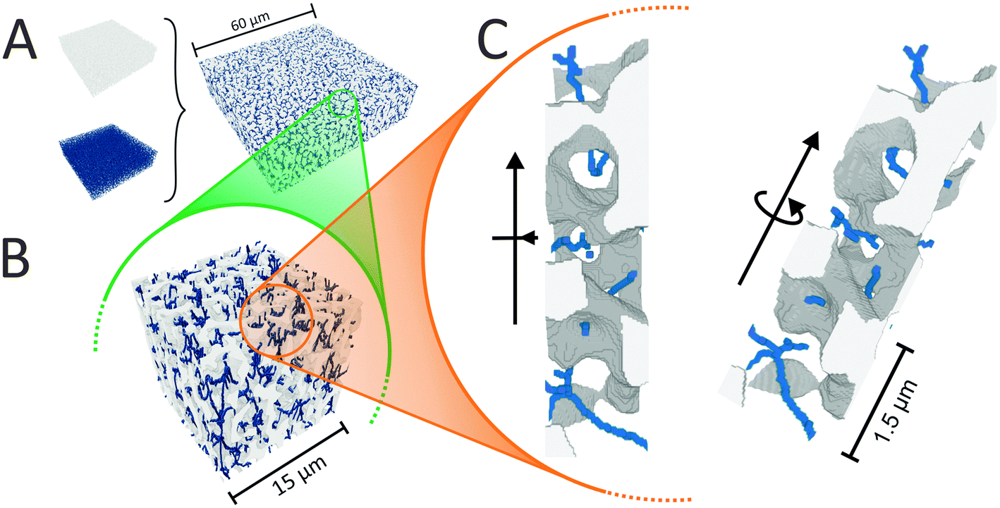

Fig. 2 (A) The reconstructed macropore space of a silica monolith (white – silica skeleton) and its medial axis (blue) are combined to illustrate how MAA works. Higher magnifications (B and C) make the character of the medial axis visible. The medial axis permeates the entire pore space, the number of branches that meet at a junction indicates the local pore connectivity.

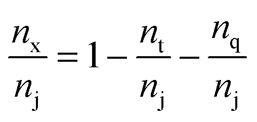
The number of branches that originate from a junction (a node of the medial axis) quantifies the local branch connectivity, which is interpreted as the local pore connectivity without ever defining the limits of individual pores. According to MAA, the investigated silica monoliths share a highly similar distribution of the local pore connectivity (Table 2). The vast majority of junctions (87–90%) connects three branches (i.e., the minimal number of branches that defines a junction), about 10% of junctions connect four branches, and higher-order junctions are scarce (1–2%). Highly similar distributions were found for other silica monoliths with comparable μ_macro-values,⁴³ interestingly also for the one existing example of a reconstructed mesopore space,³⁷ and for phase-separated organic–polymer mixtures in the late stage of spinodal decomposition (i.e., at a critical step of organic–polymer preparation).⁵⁴ The close agreement between the available data for silica monoliths suggests three-branch junctions as typical, four-branch junctions as already comparatively seldom, and higher-order junctions as very rare, which will inevitably result in a conservative value of Z ≈ 3 for the average pore connectivity. A closer analysis of the data in Table 2 indicates an increase of three-branch junctions and concurrent decrease of four-branch and higher-order junctions with increasing average macropore size of a silica monolith. An inverse correlation between μ_macro and the percentage of four-branch and higher-order junctions was previously shown in a study of eight silica monolith samples that covered a range of μ_macro = 0.43–7.20 μm.⁴³ The sample with μ_macro = 0.43 μm (a silica monolith with unusually small macropores) had 33.4% four-branch and higher-order junctions, the sample with μ_macro = 7.20 μm (a silica monolith with unusually large macropores) had 10.9% four-branch and higher-order junctions; the samples with μ_macro = 2.48 and 4.14 μm had 14.4% and 12.1% four-branch and higher-order junctions, respectively, highly similar to the percentages determined in the present study for monolith samples #1 (μ_macro = 2.54 μm, 13.2%) and #3 (μ_macro = 4.00 μm, 11.3%). The higher percentage of four-branch and higher-order junctions in monoliths with smaller macropore size raised their average pore connectivity slightly, with a maximum value of Z_av = 3.47 observed for the silica monolith sample with μ_macro = 0.43 μm. The monolith samples with typically sized macropores had values of Z_av = 3.14 and 3.17, highly similar to the values in Table 2. Our study features a smaller range of macropore sizes than the earlier one,⁴³ because we focus on commercial silica monoliths for analytical HPLC columns; accordingly, the pore connectivity varies only very slightly over our sample set. The finely structured monolith #1 (μ_macro = 2.54 μm) has only 2% more four-branch and higher-order junctions than the coarser monolith #4 with nearly twice the average macropore size (μ_macro = 4.93 μm).

Table 2 Results of MAA. Fraction of nodes in the medial axis network connecting 3, 4, or >4 branches (n_t/n_j, n_q/n_j and n_x/n_j, respectively) as well as the resulting average pore connectivity (Z). The average branch tortuosity (〈τ_branch〉) indicates the average crookedness of the branches in the medial axis network

μ macro (μm)	n t/nj	n q/nj	n x/nj	Z	〈τbranch〉
2.54	0.868	0.112	0.020	3.15	1.18 ± 0.13
3.35	0.886	0.098	0.016	3.13	1.18 ± 0.12
4.00	0.887	0.098	0.015	3.13	1.18 ± 0.14
4.93	0.892	0.093	0.015	3.12	1.18 ± 0.11

---

3.3 Topological analysis by a maximum inscribed spheres approach

The interstitial pore space of mechanically stable, random sphere packings, which are the paradigm for HPLC columns or packed beds in general, consists of larger voids connected through smaller channels. Individual pore limits can be set through tessellation schemes, for example, by using the spheres' centers for a neat division of the space into polyhedra that contain void space (pore) enclosed by solid phase (spheres).⁸⁶ The continuous solid phase of a silica monolith, on the other hand, does not lend itself to tessellation schemes. To arrive at a similarly clear-cut representation of the open macropore space, we supplemented the natural borders made by the solid phase (solid–void borders) with calculated boundaries in the macropore space (void–void borders). To maintain the analogy to the pore space of random sphere packings and to pore network models, we will refer to these calculated boundaries as pore throats.

The delineation of individual pore limits was based upon the inscription of maximum spheres into the open macropore space. For each void voxel, the smallest distance to the solid phase was determined through Euclidean distance transform. This distance is the radius of the largest (maximum) sphere around this void voxel that can be inscribed into the macropore space. The resulting set of inscribed spheres was reduced to a smaller set of containing spheres by assigning each void voxel the radius of the largest sphere in which it is contained. The resulting field of containing sphere radii contained plateaus (local maxima). The centers of containing spheres located at local maxima were used as seed points for pore propagation. In this step, all void voxels were assigned as either belonging to a certain pore or as void space shared by several pores based on the value of their assigned containing sphere radius. At this processing stage, the shared pore volumes were often as large as or even larger than that of pores. The final step propagated the pore boundaries to reduce shared pore volumes to single-voxel thick boundary layers by watershed segmentation. The identified boundaries are the watershed between individual pores at whose centers the imagined water sources are located. Harking back to maximum sphere inscription, the centers of the final pores correspond to local maxima and the calculated boundaries to local minima in the field of solid–void distances.

Fig. 3 illustrates the separate processing steps taken to compartmentalize the reconstructed macropore space of a silica monolith into a set of individual pores delimited by pore throats. The compartmentalized macropore space (Fig. 3E) differs substantially from conventional pore network models, which feature spherical or cylindrical pores homogeneously connected by cylindrical tubes (pore throats). The image in Fig. 3E shows a void space laid out in irregularly shaped and differently sized allotments, bordered by slightly curved channels (the pore throats), and interspersed with likewise irregularly shaped and differently sized patches of solid phase (the silica skeleton).

Fig. 3 Image processing steps taken to compartmentalize the open macropore space of a silica monolith into individual pores delimited by single-voxel-thick boundaries. (A) The segmented image of the reconstructed macropore space: white – silica skeleton, black – void space. (B) Through Euclidean distance transform each void voxel is assigned the radius of the largest (maximum) sphere that can be inscribed around this voxel into the void space: white – silica skeleton, color – radius of maximum sphere; color coding runs from blue (small radii) to red (large radii). (C) For each void voxel the largest containing sphere is found: white – silica skeleton, color – radius of containing sphere; color coding runs from blue (small radii) to red (large radii). (D) Through pore propagation from the local maxima of containing sphere radii, void voxels are assigned as either belonging to a certain pore (shades of blue) or as shared by several pores (black). (E) Watershed segmentation expands pores (blue) to their final size and reduces shared areas to single-voxel thick pore throats (black).

Contrary to conventional pore network models, where pore volume is quantified by the sphere or cylinder diameter (which are then collected into a pore size distribution), Fig. 3E does not suggest a comparably simple relation between size and volume for the irregularly-shaped macropore compartments. But their volume can be accurately determined by simply counting the voxels belonging to each compartment. Fig. 4A displays the resulting pore volume distributions for the four silica monoliths. The data follow the same trend as the macropore CLDs (Fig. 1B), that is, the average pore volume increases with μ_macro (Table 3). The upper pore volume limit increases from 106 μm³ for μ_macro = 2.54 μm over 201 μm³ for μ_macro = 3.55 μm and 280 μm³ for μ_macro = 4.00 μm to 519 μm³ for μ_macro = 4.93 μm. Fig. 4B shows the pore volume distributions normalized to the respective average pore volume (〈V_pore〉). The normalized distributions reveal that smaller pore volumes relative to the average pore volume appear with higher frequency in a monolith with a finer structure than in a monolith with a coarser structure but the same external porosity.

Fig. 4 (A) Distribution of pore volumes as determined by MISA. (B) Pore volume distributions normalized by the respective average pore volume 〈V_pore〉 (cf.Table 3).

Table 3 Results of MISA. Average pore volume, volume of the largest sphere that can be inscribed into the macropore space, as well as average pore and pore throat coordination numbers (C_p and C_t, respectively)

μ macro (μm)	〈Vpore〉 (μm^3)	V sphere,max (μm^3)	〈Vpore〉/Vsphere,max	C p	C t
2.54	11.92	2.17	5.49	10.6 ± 5.3	2.70 ± 0.58
3.35	23.45	4.55	5.15	10.4 ± 5.3	2.60 ± 0.58
4.00	34.51	7.10	4.86	10.1 ± 5.3	2.65 ± 0.58
4.93	57.90	11.09	5.22	11.1 ± 5.7	2.67 ± 0.59

---

Table 3 compares the average pore volume to the volume of the largest inscribed sphere (the largest sphere that can be inscribed into the void space). The data show that the average pore volume increases with μ_macro and is consistently about five times larger than the volume of the largest inscribed sphere. This observation mirrors the constant ratio between average macropore size and skeleton thickness as obtained from CLD analysis of the reconstructed macropore space (cf.Table 1).

After this short excursion into the geometrical properties of the compartmentalized macropore space, we return to the focus of our study, the pore interconnection. We determined the pore coordination by counting the number of neighbors with which a given pore shares throat voxels. Fig. 5A shows the resulting pore coordination number distributions for the four silica monoliths, which look highly similar. According to the pore coordination data every compartment functions as a central hub from which most of the surrounding compartments are accessible. 71–74% of pores are coordinated by five to fifteen neighbors. The average pore coordination number is C_p = 10–11 (Table 3), which is clearly beyond the pore coordination of the frequently used cubic network model (C_p = 6). Pore coordination numbers ≥20 are less frequent, although a small fraction of pores (5–8%) shares throat voxels with up to 35 neighbors. At first glance, these high coordination numbers seem to conflict with the average pore connectivity of Z ≈ 3.1 determined by MAA. Pore coordination number and pore connectivity, however, describe different properties and should not be confused. The pore connectivity is a measure for the branching of pores in a skeletonized representation of the macropore network. The pore coordination number refers to the compartmentalized representation of the macropore space and measures the number of pores with which a given pore shares throat voxels. The latter principle is illustrated in Fig. 5B, where the pore under consideration (colored green) shares throat voxels with six neighbors (colored in shades of yellow to tangerine). The pore coordination number is comparatively small in this example because only two dimensions were taken into account; the calculations of pore coordination for the distributions in Fig. 5A were carried out in three dimensions. Note that a pore that is separated from the center pore by the solid phase, for example, the pore between pores 5 and 6 in Fig. 5B, does not count towards the pore coordination number, as the latter's definition refers to access through advective flow. Solid phase borders can be crossed by diffusion through the mesoporous silica skeleton.

Fig. 5 (A) Distribution of pore coordination numbers as derived by MISA. The four silica monoliths share highly similar distributions with close to 75% of pores surrounded by 5–15 neighbors; 5–8% of pores have ≥20 neighbors. (B) 2D view (slice) of a compartmentalized macropore space (white – silica skeleton, black – pore throats, color – pores). The central pore (green) in the image shares throat pixels with six neighbors (yellow to tangerine). Pores that do not share throat pixels with the central pore are colored in shades of blue. In the 3D reconstruction, the central pore is coordinated by ten neighbors.

Fig. 6 illustrates how pore coordination in the compartmentalized macropore space looks like in 3D. By leaving the solid phase invisible, Fig. 6 provides an unobstructed view of the void space. The 3D image shows five directly neighbored pores and their delimiting pore throats, which are actually curved boundary layers separating individual pores. This is best visible at the pores' outer surfaces where the boundaries with further adjacent pores (that are not part of this image) are indicated. The central pore in Fig. 6 (light green) is not rimmed in red, because in the view provided by Fig. 6 this pore is hidden behind solid phase.

Fig. 6 Close-up, 3D view of a compartmentalized macropore space. Shown are five pores (pale blue, true blue, yellow, dark green, and light green) and their delimiting pore throats (red). Solid phase is not shown. Red patches at the outer surfaces of pores indicate the boundaries with adjacent pores in the compartmentalized macropore space.

Since pore throats are the connecting element in the compartmentalized representation of the macropore space, we evaluated the pore interconnection also from the perspective of the pore throats. By counting the number of pores that shared a particular throat, we received the pore throat coordination distributions for the four silica monoliths (Fig. 7). 50–57% of pore throats are shared by three pores, 37–45% by two pores, and only 5–7% by four pores. On average a particular throat coordinates C_t ≈ 2.7 pores (Table 3), a value that approaches the average pore connectivity (the average number of branches meeting at a junction) of Z ≈ 3.1 determined by MAA. The average pore connectivity cannot be smaller than three, because three is the minimum number of branches required for a junction. A throat between two pores (which may be seen as a constriction) is interpreted as a pore boundary by watershed segmentation, whereas MAA registers the same structural feature as a single pore.

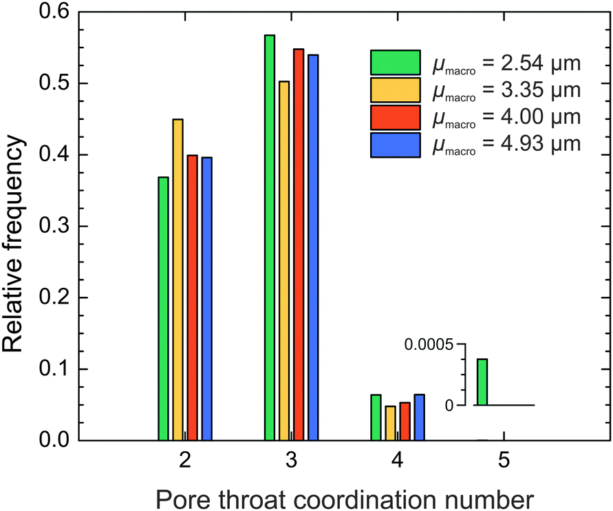Fig. 7 Distribution of pore throat coordination numbers as derived by MISA. The four silica monoliths have highly similar distributions. On average, a throat is shared by 2.7 pores. The inset shows that a five-pores coordinating throat appears with 0.04% frequency in the monolith with the finest structure.

3.4 Determination of the global geometric tortuosity by geodesic distance propagation

Solute molecules percolating through porous solids are forced to take a detour from the direct straight line when the latter is blocked by the material itself. The global geometric tortuosity defines how much longer, on average, the molecule's pathway is compared with the direct Euclidean distance.^85,87 Combined with porosity, the tortuosity defines the effective diffusivity of a solute within a porous medium and is therefore an important parameter for the mass transfer properties of a material.^86–89

To determine the global geometric tortuosity of the macropore space of a silica monolith, we extracted the geodesic distances between the center of a reconstructed volume and any void voxel in the 3D image through a voxel-by-voxel propagation. The geodesic distance gives the shortest path on which any particular void voxel can be reached from the center point without once crossing the solid–void interface. Fig. 8 illustrates the geodesic distance extraction for the monolith with the finest structure among the four samples (μ_macro = 2.54 μm).

Fig. 8 Schematic overview of geodesic distance extraction. (A) Corner-cut representation of the reconstructed macropore space of a silica monolith (white – silica skeleton). The starting point of the propagation is indicated. (B) The geodesic distances in the map for the entire reconstructed volume are color-coded from deep blue (short distances) to deep red (long distances). (C) Flat view of the faces of the cut-out corner. Geodesic distances are radially homogeneous around the center point, indicating a highly isotropic structure.

Fig. 9 summarizes the geodesic distances of the center slice plotted versus the Euclidean distance for the four silica monoliths. The strictly linear behavior of the plots confirms the validity of eqn (5) for determining global geometric tortuosity values in the reconstructed volumes of the silica monolith samples.⁸⁵ The derived value of τ_geo = 1.09 is constant within our sample set, as expected from the highly similar porosity, pore connectivity, pore coordination, and pore throat coordination data determined for the four silica monoliths.

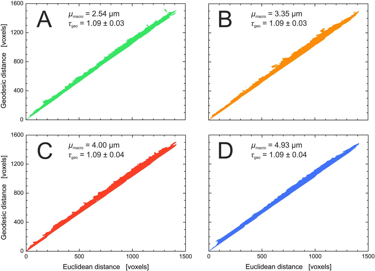Fig. 9 Geodesic distances plotted against the corresponding Euclidean distances as determined in the reconstructed macropore space. The global geometric tortuosity is represented by the slope of a corresponding linear fit (cf.eqn (5)). The four silica monoliths share a global geometric tortuosity value of 1.09. The consistently small standard deviation of the linear fits demonstrates the high isotropy of the monolithic structures.

Additionally, we determined geometric tortuosity values by MAA as the ratio of the length of a branch between two nodes to the Euclidean distance between these nodes (cf.eqn (4)). Thus, the geometric branch tortuosity measures the crookedness of a branch of the medial axis network. A point-like tracer would travel on this path when keeping an equal distance from the surrounding silica walls. An average branch tortuosity of 1.18 (with a standard deviation of ≤0.04) was found for all four silica monoliths, reflecting rather straight pathways (cf.Table 2). In an earlier study of eight silica monoliths, comprising five samples with μ_macro < 1 μm and three samples with μ_macro = 2.48–7.20 μm, average branch tortuosities between 1.23 and 1.19 were found for monoliths with supra-μm macropores and slightly higher values between 1.24 and 1.28 for the monoliths with sub-μm macropores.⁴³ Judging from the available experimental data, the branch tortuosity is a relatively stable parameter in silica monoliths and rather insensitive to the average macropore size.

Fig. 10 illustrates why the global geometric tortuosity determined from geodesic distance propagation is a bit smaller than the average geometric branch tortuosity obtained by MAA. The geodesic distance refers to the shortest possible route from point A to B in the void space, which may involve touches with the solid–void border, whereas a branch of the medial axis sticks to the middle of the road in going from point A to B.

Fig. 10 Schematic illustration of the different lengths generated by the methods used in this work: medial axis branch length d_i (aqua), geodesic distance d_geo (red), and Euclidean distance d_Euclid (green). Because the medial axis path d_i between points A and B is longer than the geodesic distance d_geo, the average branch tortuosity value determined by MAA is larger than the global geometric tortuosity.

Any geometric tortuosity value must be smaller than a tortuosity value related to actual mass transport. Solute molecules diffusing through the macropore space, for example, will experience more obstruction than expected from the geometric tortuosity values, not only because Brownian (erratic) motion leads solute molecules to deviate from the ideal route, but also because solute molecules are sensitive to constrictions in their diffusive path. Diffusive tortuosity values can be derived by numerical simulations in the reconstructed macropore space. With a random-walk particle-tracking approach and an idealized representation of solute molecules as point-like tracers, diffusive tortuosities of 1.37, 1.38, and 1.47 were found for first- and second-generation silica monoliths with external porosities of ε_ext = 0.73, 0.72, and 0.68, respectively.^47,50 The geometric tortuosity should thus be considered as the lower bound for any type of mass-transport related tortuosity.⁸⁷

4 Conclusions

Morphological analysis based on physical reconstruction has become a powerful way to obtain accurate information about the properties of random porous materials. We used physical reconstruction by confocal laser scanning microscopy to evaluate the macropore space topology of four silica monoliths. We applied and compared different approaches to quantify the pore connectivity, the pore and pore throat coordination, and the geometric tortuosity. Medial axis analysis of the macropore space yielded a branch-node network with a typical and average connectivity of three branches per node and an average geometric branch tortuosity of 1.18. The maximum inscribed spheres approach provided a compartmentalized representation of the macropore space in which individual pores are delimited by pore throats. More than 70% of pores have between five and fifteen neighbors, yielding an average pore coordination number between ten and eleven; a small fraction of pores (<10%) has fairly large coordination numbers (up to 35). The pore coordination data show each pore as a possible starting point from which most of the surrounding pores are accessible through hydrodynamic flow. The pores are reached via throats of much lower coordination. More than 50% of throats coordinate three pores, ∼40% of pores coordinate two pores, and less than 10% coordinate four pores. The average pore throat coordination number of 2.7 in the compartmentalized representation of the macropore space agrees well with the average pore (branch) connectivity of 3.1 determined by medial axis analysis. Calculating the geodesic distance between the center point and every void voxel within a reconstructed volume via a propagation algorithm yielded a global geometric tortuosity value of 1.09 for all silica monoliths. The low geometric tortuosity values reflect a very open macropore space that provides little obstruction to percolation. The geometric tortuosity values reflect the ideal route rather than the actual route that a solute molecule could take and should thus be considered as a lower bound for the diffusive (or any other mass-transport related) tortuosity. Our collected data set reveals that the four samples, whose average geometrical properties (macropore size and skeleton thickness) according to chord length distribution analysis increase by a factor of two over the set, have nonetheless highly similar topological properties (within statistical error). This observation may imply that the geometrical properties of silica monoliths can be varied over a relatively large range without impacting their topological properties.

Overall, we accomplished a comprehensive topological analysis of a non-granular, disordered porous medium, solely based on its physical reconstruction. The different analysis methods described in this work are universally applicable to porous materials, irrespective of their structure, the synthetic route by which they were prepared, and the imaging method used for their reconstruction, provided that the investigated structural features are adequately resolved. In particular, the maximum inscribed spheres approach-based compartmentalization of the open macropore space into individual pores and pore throats provides a tool to analyze the pore space of non-granular materials in the same manner as the pore space of granular materials. The received data could be used to construct new or update existing pore network models for the interpretation of physisorption and intrusion data and for simulations of application-relevant transport phenomena in silica monoliths.

Acknowledgements

This work was supported by the Deutsche Forschungsgemeinschaft DFG (Bonn, Germany) under grant TA 268/9-1.

References

1. G. Guiochon, J. Chromatogr. A, 2007, 1168, 101–168.
2. K. K. Unger, R. Skudas and M. M. Schulte, J. Chromatogr. A, 2008, 1184, 393–415.
3. Z. Walsh, B. Paull and M. Macka, Anal. Chim. Acta, 2012, 750, 28–47.
4. A. Sachse, A. Galarneau, B. Coq and F. Fajula, New J. Chem., 2011, 35, 259–264.
5. A. Sachse, V. Hulea, A. Finiels, B. Coq, F. Fajula and A. Galarneau, J. Catal., 2012, 287, 62–67.
6. A. Sachse, N. Linares, P. Barbaro, F. Fajula and A. Galarneau, Dalton Trans., 2013, 42, 1378–1384.
7. K. Nakanishi and N. Tanaka, Acc. Chem. Res., 2007, 40, 863–873.
8. S. Hartmann, D. Brandhuber and N. Hüsing, Acc. Chem. Res., 2007, 40, 885–894.
9. A. Inayat, B. Reinhardt, H. Uhlig, W.-D. Einicke and D. Enke, Chem. Soc. Rev., 2013, 42, 3753–3764.
10. C. Triantafillidis, M. S. Elsaesser and N. Hüsing, Chem. Soc. Rev., 2013, 42, 3833–3846.
11. J. Babin, J. Iapichella, B. Lefèvre, C. Biolley, J.-P. Bellat, F. Fajula and A. Galarneau, New J. Chem., 2007, 31, 1907–1917.
12. F. Gritti and G. Guiochon, J. Chromatogr. A, 2012, 1221, 2–40.
13. F. Gritti and G. Guiochon, Anal. Chem., 2013, 85, 3017–3035.
14. F. Gritti and G. Guiochon, J. Chromatogr. A, 2009, 1216, 4752–4767.
15. K. Hormann, T. Müllner, S. Bruns, A. Höltzel and U. Tallarek, J. Chromatogr. A, 2012, 1222, 46–58.
16. M. Motokawa, H. Kobayashi, N. Ishizuka, H. Minakuchi, K. Nakanishi, H. Jinnai, K. Hosoya, T. Ikegami and N. Tanaka, J. Chromatogr. A, 2002, 961, 53–63.
17. T. Hara, H. Kobayashi, T. Ikegami, K. Nakanishi and N. Tanaka, Anal. Chem., 2006, 78, 7632–7642.
18. S. Altmaier and K. Cabrera, J. Sep. Sci., 2008, 31, 2551–2559.
19. R. Skudas, B. A. Grimes, M. Thommes and K. K. Unger, J. Chromatogr. A, 2009, 1216, 2625–2636.
20. T. Hara, S. Makino, Y. Watanabe, T. Ikegami, K. Cabrera, B. Smarsly and N. Tanaka, J. Chromatogr. A, 2010, 1217, 89–98.
21. K. Cabrera, LCGC North Am., 2012, 30, 30–35.
22. K. Hormann and U. Tallarek, J. Chromatogr. A, 2013, 1312, 26–36.
23. F. Gritti and G. Guiochon, J. Chromatogr. A, 2012, 1225, 79–90.
24. M. Thommes, R. Skudas, K. K. Unger and D. Lubda, J. Chromatogr. A, 2008, 1191, 57–66.
25. A. H. Dessources, S. Hartmann, M. Baba, N. Huesing and J. M. Nedelec, J. Mater. Chem., 2012, 22, 2713–2720.
26. J. Rouquerol, G. Baron, R. Denoyel, H. Giesche, J. Groen, P. Klobes, P. Levitz, A. V. Neimark, S. Rigby, R. Skudas, K. Sing, M. Thommes and K. Unger, Pure Appl. Chem., 2012, 84, 107–136.
27. M. Thommes and K. A. Cychosz, Adsorption, 2014, 20, 233–250.
28. G. Möbus and B. J. Inkson, Mater. Today, 2007, 10, 18–25.
29. P. Levitz, Cem. Concr. Res., 2007, 37, 351–359.
30. L. Karwacki, D. A. M. de Winter, L. R. Aramburo, M. N. Lebbink, J. A. Post, M. R. Drury and B. M. Weckhuysen, Angew. Chem., Int. Ed., 2011, 50, 1294–1298.
31. H. Schulenburg, B. Schwanitz, N. Linse, G. G. Scherer, A. Wokaun, J. Krbanjevic, R. Grothausmann and I. Manke, J. Phys. Chem. C, 2011, 115, 14236–14243.
32. H. Koku, R. S. Maier, M. R. Schure and A. M. Lenhoff, J. Chromatogr. A, 2012, 1237, 55–63.
33. E. A. Wargo, T. Kotaka, Y. Tabuchi and E. C. Kumbur, J. Power Sources, 2013, 241, 608–618.
34. A. P. Cocco, G. J. Nelson, W. M. Harris, A. Nakajo, T. D. Myles, A. M. Kiss, J. J. Lombardo and W. K. S. Chiu, Phys. Chem. Chem. Phys., 2013, 15, 16377–16407.
35. S. J. Harris and P. Lu, J. Phys. Chem. C, 2013, 117, 6481–6492.
36. T. Müllner, A. Zankel, F. Svec and U. Tallarek, Mater. Today, 2014, 17, 404–411.
37. D. Stoeckel, C. Kübel, K. Hormann, A. Höltzel, B. M. Smarsly and U. Tallarek, Langmuir, 2014, 30, 9022–9027.
38. P. Aggarwal, V. Asthana, J. S. Lawson, H. D. Tolley, D. R. Wheeler, B. A. Mazzeo and M. L. Lee, J. Chromatogr. A, 2014, 1334, 20–29.
39. T. Müllner, A. Zankel, Y. Lv, F. Svec, A. Höltzel and U. Tallarek, Adv. Mater., 2015, 27, 9009–9013.
40. K. Kanamori, H. Yonezawa, K. Nakanishi, K. Hirao and H. Jinnai, J. Sep. Sci., 2004, 27, 874–886.
41. H. Saito, K. Nakanishi, K. Hirao and H. Jinnai, J. Chromatogr. A, 2006, 1119, 95–104.
42. H. Saito, K. Kanamori, K. Nakanishi and K. Hirao, J. Sep. Sci., 2007, 30, 2881–2887.
43. D. Stoeckel, C. Kübel, M. O. Loeh, B. M. Smarsly and U. Tallarek, Langmuir, 2015, 31, 7391–7400.
44. S. Bruns, T. Müllner, M. Kollmann, J. Schachtner, A. Höltzel and U. Tallarek, Anal. Chem., 2010, 82, 6569–6575.
45. S. Bruns and U. Tallarek, J. Chromatogr. A, 2011, 1218, 1849–1860.
46. S. Bruns, J. P. Grinias, L. E. Blue, J. W. Jorgenson and U. Tallarek, Anal. Chem., 2012, 84, 4496–4503.
47. D. Hlushkou, S. Bruns, A. Höltzel and U. Tallarek, Anal. Chem., 2010, 82, 7150–7159.
48. D. Hlushkou, S. Bruns, A. Seidel-Morgenstern and U. Tallarek, J. Sep. Sci., 2011, 34, 2026–2037.
49. A. Daneyko, A. Höltzel, S. Khirevich and U. Tallarek, Anal. Chem., 2011, 83, 3903–3910.
50. D. Hlushkou, K. Hormann, A. Höltzel, S. Khirevich, A. Seidel-Morgenstern and U. Tallarek, J. Chromatogr. A, 2013, 1303, 28–38.
51. S. Bruns, T. Hara, B. M. Smarsly and U. Tallarek, J. Chromatogr. A, 2011, 1218, 5187–5194.
52. S. Bruns, E. G. Franklin, J. P. Grinias, J. M. Godinho, J. W. Jorgenson and U. Tallarek, J. Chromatogr. A, 2013, 1318, 189–197.
53. Z. Liang, M. A. Ioannidis and I. Chatzis, J. Colloid Interface Sci., 2000, 221, 13–24.
54. H. Jinnai, H. Watashiba, T. Kajihara and M. Takahashi, J. Chem. Phys., 2003, 119, 7554–7559.
55. Y. Yao, K. J. Czymmek, R. Pazhianur and A. M. Lenhoff, Langmuir, 2006, 22, 11148–11157.
56. P. Levitz, V. Tariel, M. Stampanoni and E. Gallucci, Eur. Phys. J.: Appl. Phys., 2012, 60, 24202.
57. D. Silin and T. Patzek, Physica A, 2006, 371, 336–360.
58. A. S. Al-Kharusi and M. J. Blunt, J. Pet. Sci. Eng., 2007, 56, 219–231.
59. H. Dong and M. J. Blunt, Phys. Rev. E: Stat., Nonlinear, Soft Matter Phys., 2009, 80, 036307.
60. A. P. Jivkov, C. Hollis, F. Etiese, S. A. McDonald and P. J. Withers, J. Hydrol., 2013, 486, 246–258.
61. A. N. Ebrahimi, S. Jamshidi, S. Iglauer and R. B. Boozarjomehry, Chem. Eng. Sci., 2013, 92, 157–166.
62. M. Prat, Chem. Eng. Technol., 2011, 34, 1029–1038.
63. M. Siena, M. Riva, J. D. Hyman, C. L. Winter and A. Guadagnini, Phys. Rev. E: Stat., Nonlinear, Soft Matter Phys., 2014, 89, 013018.
64. C. F. Berg, Transp. Porous Media, 2014, 103, 381–400.
65. W. S. Rasband, ImageJ, U. S. National Institutes of Health, Bethesda, Maryland, USA, 1997–2015, http://imagej.nih.gov/ij/, accessed September 2015.
66. P. Levitz and D. Tchoubar, J. Phys. I, 1992, 2, 771–790.
67. S. Torquato and B. Lu, Phys. Rev. E: Stat. Phys., Plasmas, Fluids, Relat. Interdiscip. Top., 1993, 47, 2950–2953.
68. S. Torquato, Random Heterogeneous Materials: Microstructure and Macroscopic Properties, Springer, New York, 2002.
69. J. Courtois, M. Szumski, F. Georgsson and K. Irgum, Anal. Chem., 2007, 79, 335–344.
70. R. Meinusch, K. Hormann, R. Hakim, U. Tallarek and B. M. Smarsly, RSC Adv., 2015, 5, 20283–20294.
71. S. Bochkanov and V. Bystritsky, ALGLIB, http://www.alglib.net.
72. T. Aste and T. Di Matteo, Phys. Rev. E: Stat., Nonlinear, Soft Matter Phys., 2008, 77, 021309.
73. S. Bruns, D. Stoeckel, B. M. Smarsly and U. Tallarek, J. Chromatogr. A, 2012, 1268, 53–63.
74. I. Arganda-Carreras, Image Analysis, http://https://sites.google.com/site/iargandacarreras/software, accessed September 2015.
75. T.-C. Lee, R. L. Kashyap and C.-N. Chu, CVGIP: Graphical Models Image Process, 1994, 56, 462–478.
76. V. Baranau, Porous Media Analysis, http://https://github.com/VasiliBaranov/PorousMedia Analysis, accessed September 2015.
77. E. L. van den Broek and T. E. Schouten, Recent Patents Comput. Sci., 2011, 4, 1–15.
78. R. Fabbri, L. D. F. Costa, J. C. Torelli and O. M. Bruno, ACM Comput. Surv., 2008, 40(1), 2:1–2:44.
79. Y. Lucet, Image Vis. Comput., 2009, 27, 37–44.
80. C. R. Maurer, R. S. Qi and V. Raghavan, IEEE Trans. Pattern Anal. Mach. Intell., 2003, 25, 265–270.
81. A. Meijster, J. B. T. M. Roerdink and W. H. Hesselink, in Mathematical Morphology and its Applications to Image and Signal Processing, ed. J. Goutsias, L. Vincent and D. S. Bloomberg, Computational Imaging and Vision Series, Springer, US, 2000, vol. 18, pp. 331–340.
82. A. Bieniek and A. Moga, Pattern Recognit., 2000, 33, 907–916.
83. F. Meyer, Signal Process., 1994, 38, 113–125.
84. T. H. Cormen, C. E. Leiserson, R. L. Rivest and C. Stein, Introduction to Algorithms, The MIT Press, London, 2009.
85. C. J. Gommes, A.-J. Bons, S. Blacher, J. H. Dunsmuir and A. H. Tsou, AIChE J., 2009, 55, 2000–2012.
86. S. Khirevich, A. Höltzel, A. Daneyko, A. Seidel-Morgenstern and U. Tallarek, J. Chromatogr. A, 2011, 1218, 6489–6497.
87. B. Ghanbarian, A. G. Hunt, R. P. Ewing and M. Sahimi, Soil Sci. Soc. Am. J., 2013, 77, 1461–1477.
88. L. Shen and Z. Chen, Chem. Eng. Sci., 2007, 62, 3748–3755.
89. M. Letellier, V. Fierro, A. Pizzi and A. Celzard, Carbon, 2014, 80, 193–202.

---