
Optofluidic tunable lenses using laser-induced thermal gradient†
Qingming
Chen
ab,
Aoqun
Jian
c,
Zhaohui
Li
*d and
Xuming
Zhang
*ab
aShenzhen Research Institute, Shenzhen, PR China
bDepartment of Applied Physics, The Hong Kong Polytechnic University, Hong Kong, People's Republic of China. E-mail: apzhang@polyu.edu.hk; li_zhaohui@hotmail.com; Fax: 852 23337629; Tel: 852 34003258
cMicroNano System Research Center, College of Information Engineering, Taiyuan University of Technology, Taiyuan 030024, People's Republic of China
dInstitute of Photonics Technology, Jinan University, Guangzhou 510632, People's Republic of China
First published on 9th November 2015
Abstract
This paper reports a new design of optofluidic tunable lens using a laser-induced thermal gradient. It makes use of two straight chromium strips at the bottom of the microfluidic chamber to absorb the continuous pump laser to heat up the moving benzyl alcohol solution, creating a 2D refractive index gradient in the entrance part between the two hot strips. This design can be regarded as a cascade of a series of refractive lenses, and is distinctively different from the reported liquid lenses that mimic the refractive lens design and the 1D gradient index lens design. CFD simulation shows that a stable thermal lens can be built up within 200 ms. Experiments were conducted to demonstrate the continuous tuning of focal length from initially infinite to the minimum 1.3 mm, as well as the off-axis focusing by offsetting the pump laser spot. Data analyses show the empirical dependences of the focal length on the pump laser intensity and the flow velocity. Compared with previous studies, this tunable lens design enjoys many merits, such as fast tuning speed, aberration-free focusing, remote control, and enabling the use of homogeneous fluids for easy integration with other optofluidic systems.
1. Introduction
The synergy of light and fluid has a long history. Early examples may be traced back to Fizeau's experiment1 for determining the speed of light in running water in 1851 and the light fountains2 invented not later than 1880. Recently, the development of microfluidic technology gave birth to a new research field called “optofluidics”,3–10 which integrates light and fluids into a microscale platform for advanced optical and photonic functionalities. In a short span of time, optofluidics has made tremendous progress and it is still driving a paradigm shift in many areas that involve fluids and light, such as biochemical analyses,6,8,11–14 energy production,5,15–18 light sources19–23 and many other optical systems.7,24–32 In these optofluidic systems, it is essential to focus the light to a desired location in a controllable manner for optical coupling,32 switching,33–36 collection11–13,37 and trapping.38–40 In fact, many optofluidic systems are arranged in the same plane (i.e., very thin in the vertical direction) and the function of in-plane focusing is already good enough for many application scenarios.38–40Various optofluidic designs have been developed for in-plane focusing,28 but they can be broadly classified into two categories: refractive lens design and one-dimensional gradient index (1D-GRIN) lens design, as shown in Fig. 1. The refractive lens design mimics the concept of conventional solid focal lenses with curved interfaces, as illustrated in Fig. 1(a). It typically creates curved interfaces using immiscible fluids of different refractive indices (RI) and has a step change of RI across each interface. Prominent examples are the liquid-core liquid-cladding tunable lenses, which run a high-RI core flow sandwiched by two low-RI cladding flows in a narrow microchannel.41–47 In an expanded region of the microchannel, the core and cladding flows rearrange themselves to form curved interfaces, dependent on the hydrodynamic pressures and thus the pumping flow rates. In contrast, the 1D-GRIN lens design mimics the concept of conventional solid GRIN lenses (see Fig. 1(b)), and commonly generates a continuous change of the RI by mixing miscible fluids of different RIs48 or by introducing a temperature gradient in a homogeneous fluid.49 In the ideal case, the equi-RI lines are all straight and parallel to the optical axis (see Fig. 1(b)). In reality, the equi-lines may be slightly curved but are still approximately parallel. Mao et al. pioneered this concept using CaCl2 solution (n = 1.41) and water (n = 1.33) as the core and the cladding, respectively.48 The intermixing of the two types of flows generates a hyperbolic secant profile of RI and thus a GRIN lens. Different levels of focusing have been demonstrated. In addition to the focusing effect, the GRIN-lens design has also been used for large-angle bending and splitting of light.34,50 These two categories of designs have been well developed for the in-plane focusing function, but the demonstrated studies still have some constraints. One is that the tuning of the focusing state is mostly by adjusting the flow rates. Due to the viscous nature of fluids and the long fluidic connection from the external flow pumps, the tuning response is usually slow (∼1 s).28 The other is that the adjustment through the external flow pumps modifies the whole optofluidic waveguide and provides no freedom to relocate the lens to another point of interest.
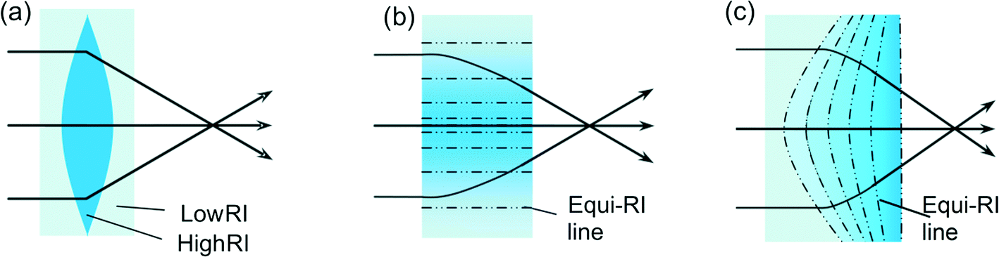 | ||
| Fig. 1 Working principles of two typical designs and our new design of an optofluidic lens. (a) Refractive lens design, which mimics the concept of conventional solid curved-interface lenses and utilizes immiscible flows with different refractive indices to create curved interfaces. The focusing effect is obtained by the sharp bending of the rays at the curved interfaces of two homogeneous media. (b) 1D-GRIN lens design, which mimics the concept of conventional solid GRIN lenses, which have a parabolic distribution refractive index in the transverse direction and the equi-RI lines parallel to the central line. The continuous change of the RI is obtained by mixing miscible fluids of different RIs or by introducing a temperature gradient in a homogeneous fluid. The rays are bent inwards gradually. (c) New 2D-GRIN lens design, which has the gradient index changes in both the longitudinal and transverse directions. The equi-RI lines are curved, making it like the cascade of many refractive lenses along the optical axis. This design can be regarded as a combination of the refractive lens design and the GRIN-lens design. | ||
In this paper, we will present another design of optofluidic tunable lens, which can be regarded as a combination of the previous two designs (see Fig. 1(c)) and is realized by using the laser-induced thermal gradient. It is able to overcome the existing constraints and brings additional benefits. Detailed discussions on the working principle, the device design and the experimental results will be presented below, followed by some discussions.
2. Concept and theory
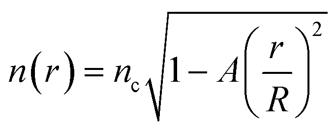
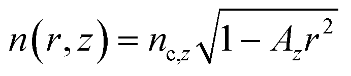
The conceptual design of the new type of optofluidic lens is shown in Fig. 1(c). It has refractive index (RI) gradient changes in both the longitudinal and the transverse directions (called a 2D-GRIN lens), thus the equi-RI lines are in a curved shape. These features are distinctively different from the typical 1D-GRIN lens design, which has the RI gradient only in the transverse direction and has the equi-RI lines in a straight shape. Compared with the typical refractive lens design, the 2D-GRIN lens design looks like the cascade of a series of refractive lenses along the optical axis. Simply speaking, the focusing effect of the 2D-GRIN lens design is obtained by gradually bending the rays to one point and can be tuned by varying the RI gradient profile.In theory, one of the RI gradient profiles that can realize aberration-free focusing should follow the square-law parabolic function as given by,
 | (1a) |
 | (1b) |
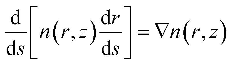
In the 2D space, the ray trajectories inside an optical medium are determined by
 | (2) |
The tuning of RI can be obtained by varying the temperature. According to the thermo-optics effect, the RI of a liquid is a function of the temperature as approximated by51
 | (3) |
In this work, CFD (computational fluidic dynamics) and optical ray tracing simulations are conducted to find an optimized design of tunable liquid lens. First, a CFD programme is conducted to calculate the heat transfer by considering the microchip geometry and the flow parameters. Then, the temperature field is converted into a temperature-induced RI gradient field. Finally, we simulate the ray tracing in the RI gradient field. Experimentally, the temperature field is measured by filling the microchip with the rhodamine B fluorescence solution, whose fluorescence emission is strongly dependent on the temperature.52 More details of the simulation and the temperature measurement can be found in the ESI.†
3. Device design
The schematic design of the optofluidic tunable lens device is illustrated in Fig. 2. It consists of three separate parts: a microchip, a pump laser and an optical fiber. The microchip is the core part for fluidic control and light focusing; the pump laser is mounted above the microfluidic chip for light irradiation; and the optical fiber is used to couple the probe light into the microchip for determination of the focusing effect. The microchip has three layers in the vertical direction: the top and the bottom are silica glass slides (nsilica = 1.46), and in between is the microfluidic structural layer for a rectangular microchamber. Two inlets and two outlets are arranged symmetrically to balance the input and output of liquid. The microchamber is 5 mm long, 1.5 mm wide and 45 μm high. The height is intentionally chosen to be very small so that the flow convection in the heating process is negligible. This helps sustain the state of laminar flow even when part of the liquid is heated. The microchamber is photolithographically patterned by NOA68 optical adhesive (nNOA68 = 1.540). Two chromium straight strips (width = 125 μm, length = 1 mm, thickness = 1 μm, center-to-center separation = 375 μm) are coated on the bottom glass by magnetron sputtering as the microheaters. For the pump laser, a continuous laser from a semiconductor diode is guided through a multimode fiber (λ = 980 nm, NA = 0.22, Dcore = 200 μm) to irradiate the metal strips, whose absorption heats up the liquid to establish a sustainable temperature gradient. The pump laser fiber is mounted over the microchip and controlled by an optical stage to precisely adjust the laser spot position on the microchip. Green light (λ = 532 nm) is coupled into the microchip through a pigtailed lensed fiber collimator. Benzyl alcohol is chosen as the liquid to fill the microchamber. This is because benzyl alcohol has very low absorptions at 520 nm and 980 nm, a high thermo-optic coefficient (dn/dT = −5.1 × 10⁻⁴ K−1), a high boiling point of 203 °C, a low heat transfer coefficient and a suitable viscosity (see Supplementary section S2† for the determination of the thermo-optic coefficient of benzyl alcohol). In addition, benzyl alcohol has a RI of n = 1.5389 at 25 °C, which closely matches the RI of NOA68 adhesive (nNOA68 = 1.540) for easy optical propagation in the horizontal plane, and is higher than that of the top and bottom glass slides (nsilica = 1.46) for optical confinement in the vertical direction. For direct visualization, a CCD imaging system (not shown in Fig. 2) is introduced to capture pictures and videos from the top side for post-processing.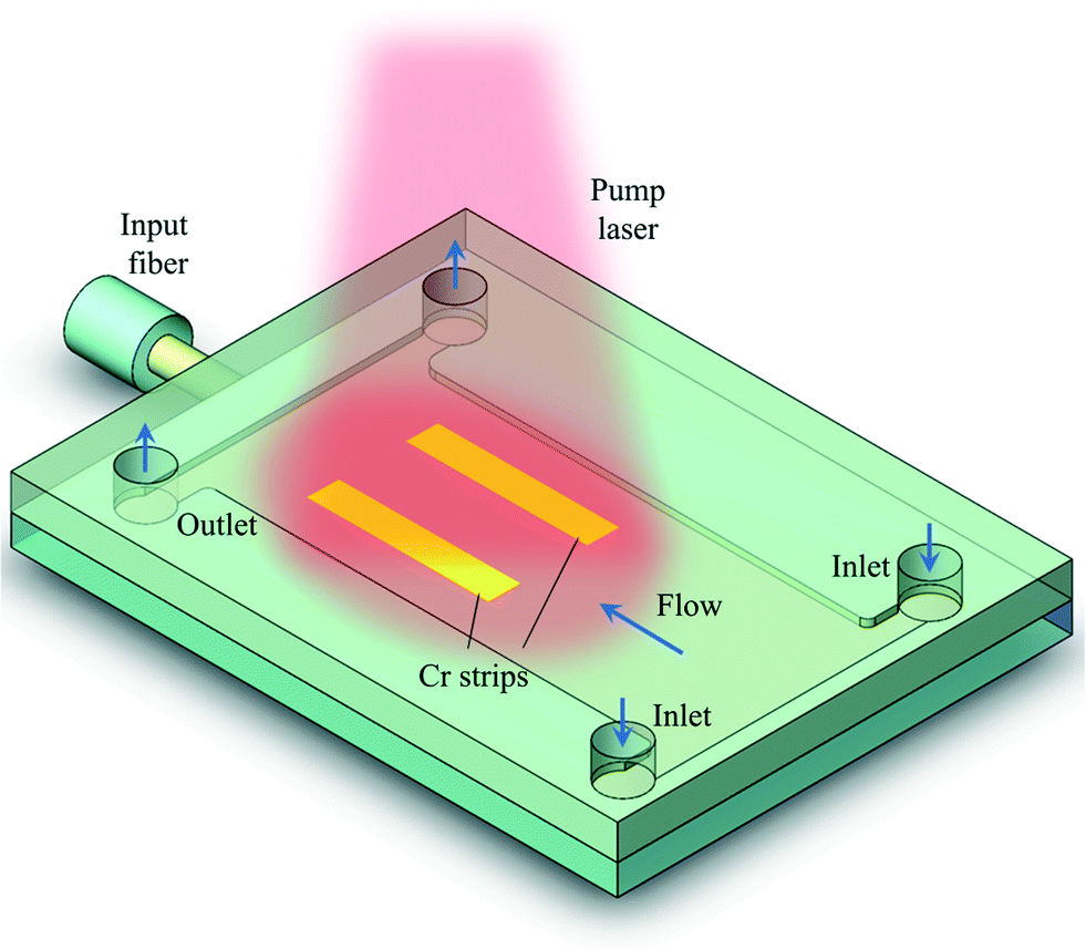 | ||
| Fig. 2 Schematic diagram of the new optofluidic tunable lens device. It has two inlets at one end and two outlets at the other end. Two silica glasses are used as the top and bottom. An NOA68 layer sandwiched by the two glasses is the spacer and the structural layer, which defines a rectangle chamber inside the chip. Two chromium strips are coated on the bottom glass to absorb the pump laser for heat generation. The heat transfer from the strips to the liquid and the motion of liquid work together to create a temperature field and thus a refractive index gradient. Under proper conditions, the refractive index gradient can focus the probe light from a fiber laser to a tunable point. | ||
4. Results and discussion
4.1 Simulated and measured refractive index gradients
The RI gradient profiles should be examined before considering the focusing effect. First, a three-dimensional (3D) computational fluidic dynamics (CFD) simulation is conducted to investigate the evolution of the RI profile inside the microchamber (see Fig. 3 and the ESI2 video in ESI†). It can be seen that it takes about 200 ms to establish a stable RI profile. More results of simulation and measurement are exemplified in Fig. 4. From the 2D RI profile in Fig. 4(a), it is seen that when the cool liquid flows through the hot strips, an RI gradient field is generated, especially at the entrance part between the two strips. The RI profile exhibits clearly curved equi-RI lines, as expected from Fig. 1(c). The RI ranges from 1.50 to 1.54 (Δn = 0.04) when the temperature is changed from 25 °C to about 85 °C. In the 3D plot in Fig. 4(b), it is seen that the RI has little change along the vertical direction. This suggests that the ray tracing simulation can be conducted in 2D, rather than 3D. Fig. 4(c) shows the RI profile measured by using the rhodamine B fluorescence. It looks very similar to the simulated field in Fig. 4(a). The RI distributions along three observation lines P1, P2 and P3 are plotted in Fig. 4(d). They all follow closely the square-law parabolic function.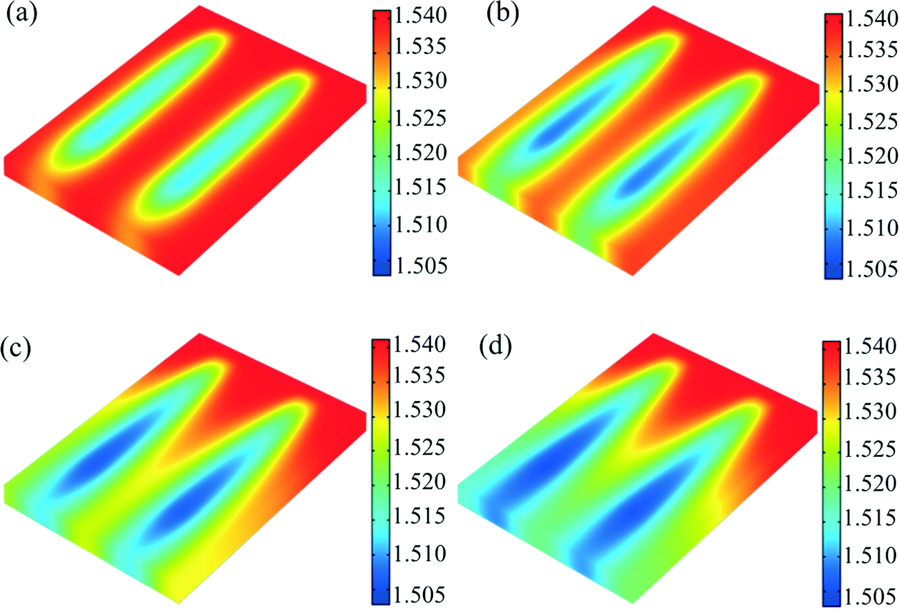 | ||
| Fig. 3 Dynamic simulation of the evolution of the refractive index gradient inside the microchamber after the pump laser is turned on. The flow velocity is v = 6.17 mm s−1 and the net pump laser intensity is Ps = 0.31 W mm−2. (a) At 25 ms, the flowing liquid close to the metal strips is heated up first. (b) After 50 ms, the refractive index along the vertical direction becomes uniform. (c) At 100 ms, a tongue-shaped refractive index profile is formed between the two strips. (d) At 200 ms, the refractive index profile becomes stable. | ||
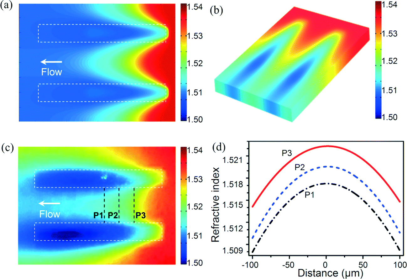 | ||
| Fig. 4 Simulation and measurement of the refractive index profile at the flow velocity v = 6.17 mm s−1. The simulated (a) two-dimensional and (b) three-dimensional refractive index profiles, the pump laser intensity in simulation Ps = 0.31 W mm−2. (c) Measured refractive index profile as determined by the temperature dependency of rhodamine B fluorescence, the pump laser intensity in experiment Pi = 0.60 W mm−2. (d) The refractive index distributions along three observation lines, which follow closely the square-law parabolic function. The white dashed rectangles in (a) and (c) represent the positions of the chromium strips. It is noted that the difference between Pi and Ps is due to the partial absorption of the laser energy by the metal strips, with an absorption efficiency of 51.7%. | ||
4.2 Tuning of focusing states
Fig. 5 demonstrates different focusing states as observed in the experiment. To visualize the light path, the benzyl alcohol solution is added with a bit of rhodamine B dye, which absorbs 532 nm light and emits yellow fluorescence for the CCD imaging. In the initial state (i.e., the pump light is turned off), the probe light is a parallel beam with width of about 250 μm (see Fig. 5(a1)). After the pump laser is turned on, the parallel input probe light starts to be focused, and the focal spot is moved from right to left with the increase of the pump intensity (see Fig. 5(a2)–(a4)). A minimum focal length of 1.3 mm is obtained under the conditions of the flow velocity v = 2.06 mm s−1 and the pump intensity Pi = 0.60 W mm−2. Further increase of the pump intensity would cause an unstable flow and thus deteriorate the focusing effect. The focusing spots in Fig. 5(a2)–(a4) are all on the optical axis as a result of symmetric irradiation of the two strips. However, when the pump spot is offset to create an asymmetric RI profile, the probe light beam can be deflected to form an off-axis focusing, as shown in Fig. 5(a5). To demonstrate the real-time tuning of the focusing state, a video can be found in the ESI.†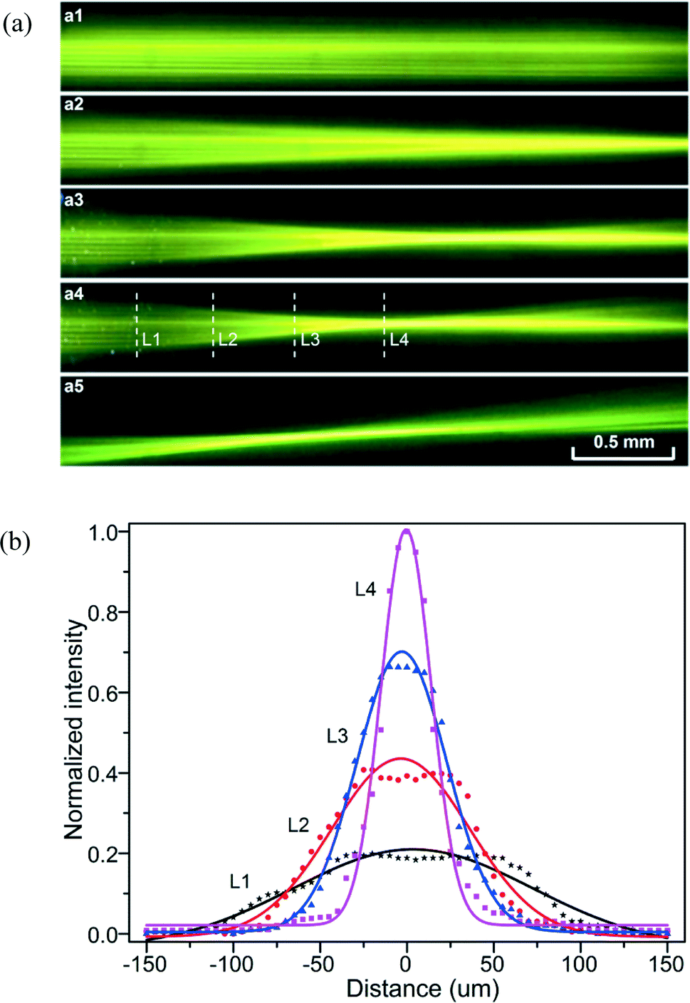 | ||
| Fig. 5 Experiments of the tunable optofluidic lens. (a) Different focal states: (a1) the initial state when the pump laser is off; (a2) focusing under laser power of 0.3 W mm−2; (a3) increased focusing under 0.5 W mm−2; (a4) further increased focusing under 0.6 W mm−2, obtaining the shortest focal length of 1.3 mm; (a5) deflection of the focused beam when the pump laser spot is moved away from the center to generate an asymmetric refractive index. (b) Normalized intensity distributions along the observation lines L1–L4. The solid curves are fitted to the Gaussian function. It is seen that the peak intensity goes higher and the curve shape approaches closer to the Gaussian function when the observation line is moved closer to the focal spot. | ||
The normalized intensity distributions along four observation lines L1 to L4 of Fig. 5(a4) are plotted in Fig. 5(b). They are fitted to the Gaussian function. It is seen that the peak intensity at the center is increased sharply and the curve shape is better fitted to the Gaussian function when the observation line moves closer to the focal spot. The theoretical value of the focal spot size should be 5.5 μm for the focal length of 1.30 mm, while the measured value is about 9.8 μm due to the enlargement from fluorescent dye (see Supplementary section S4† for more details).
4.3 Dependences of focal length on pump laser intensity and flow velocity
It is easy to understand that the focal length is dependent on two factors: the flow velocity and the pump laser intensity. To find out the empirical relationships, two sets of experiments are conducted. First, the flow velocity is maintained at v1 = 2.06 mm s−1 or v2 = 6.17 mm s−1, whereas the pump laser intensity is varied gradually from very low to the maximum 0.6 W mm−2. The results are plotted in Fig. 6(a) with error bars. Each data point represents five measurements. When the pump laser intensity is increased from about 0.4 W mm−2 to 0.6 W mm−2, the focal lengths are decreased from about 2.9 mm to 1.3 mm for v1 = 2.06 mm s−1, and 3.3 mm to 1.5 mm for v2 = 6.17 mm s−1. It was found that the two curves can be well fitted by the second-order polynomial function F(Pi) = a0 + a1Pi + a2P2i, where F is the focal length (in mm) and Pi is the pump laser intensity (in W mm−2). For the coefficients, these are a0 = 10.479, a1 = −27.368, and a2 = 20.242 for the case of v1 = 2.06 mm s−1, and a0 = 12.449, a1 = −32.905 and a2 = 24.390 for the case of v2 = 6.17 mm s−1. To verify the empirical relationship, we further simulated the relationship between the pump laser intensity and the focal length and then compared with the experimental results as detailed in Supplementary section S5.† It can be seen that the two curves match roughly with each other, as shown in Fig. S6,† after a conversion of the experimental pump laser intensity into the simulated pump laser intensity using the absorption efficiency.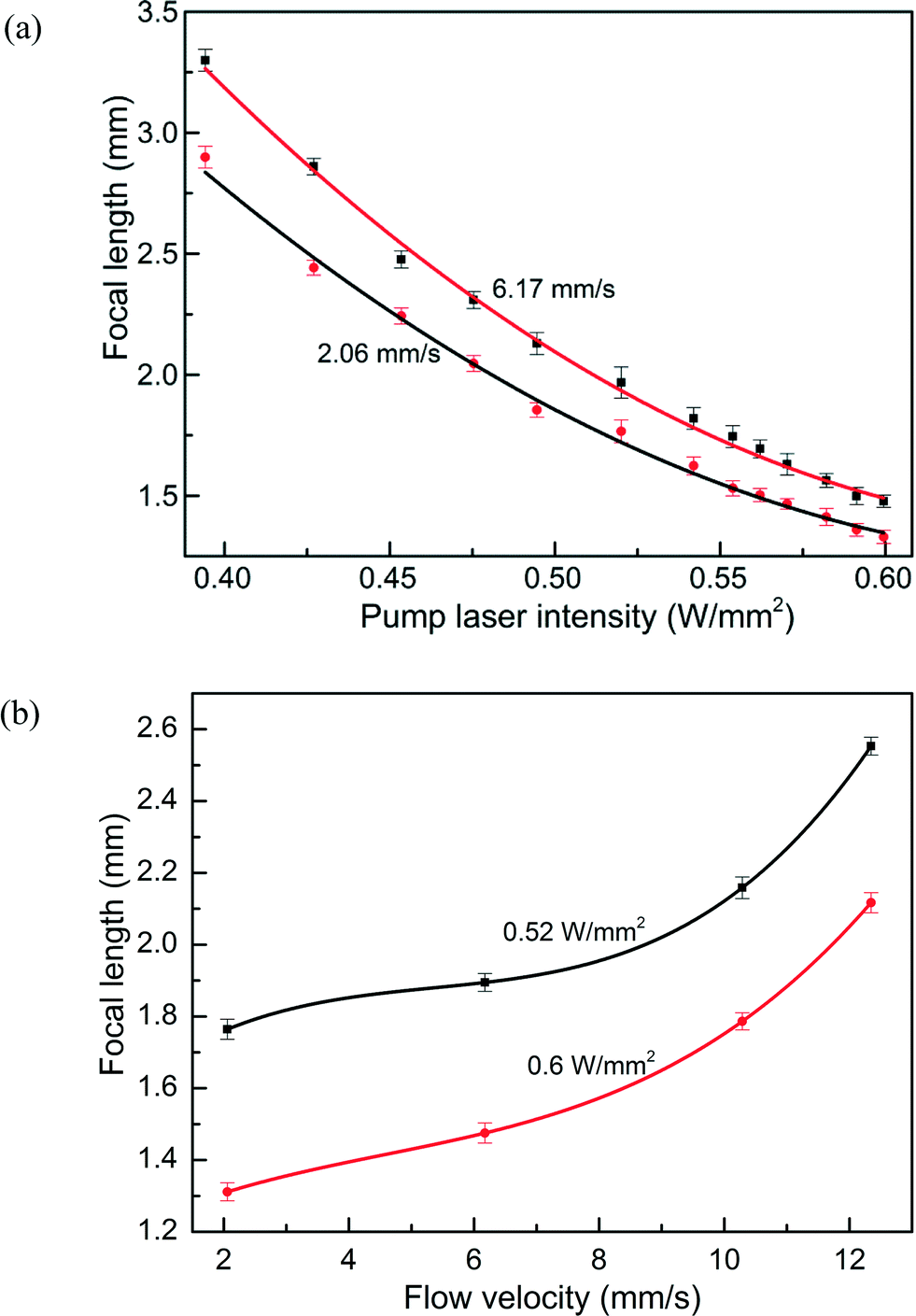 | ||
| Fig. 6 Measured tunabilities of the optofluidic lens. (a) Focal length as a function of the pump laser power under two different flow velocities. The solid curves are the fitted second-order polynomial functions. (b) Focal length as a function of the flow velocity with two constant pump powers. The solid curves are the fitted third-order polynomial functions. | ||
Similarly, the focal length as a function of the flow velocity is measured at the pump laser intensity of 0.52 W mm−2 or 0.6 W mm−2, as plotted in Fig. 6(b). The focal length goes longer when the flow is moving faster, and can be well fitted by the third-order polynomial function F(v) = b0 + b1v + b2v2 + b3v3 (F in mm and v in mm s−1). The coefficients are b0 = 1.535, b1 = 0.1577, b2 = −0.0262 and b3 = 1.630 × 10⁻³ for the case of Pi = 0.5 W mm−2, and b0 = 1.165, b1 = 0.09333, b2 = −0.01263 and b3 = 9.170 × 10⁻⁴ for the case of Pi = 0.6 W mm−2. Although the experimental data are not sufficient to derive the two-variable empirical function F(Pi,v), the empirical relationships make it feasible for the real-time tuning of the focal length.
4.4 Discussion
(1) Metal strip width: the metal strips of the working device are chosen to be 125 μm wide. As the sources of heat energy, the metal strips should have a width of 0 μm in the ideal case. However, narrow strips cause low absorption to the pump laser, whereas too wide strips would disturb the heat field. The width of 125 μm is found be to a suitable choice for our experiments.
(2) Separation of metal strips: it is 250 μm in the working device. A larger separation leads to a longer time to stabilize the temperature profile and also causes a longer focal length as the refractive index gradient is weakened (since the maximum temperature difference is determined by the boiling point of the solution). However, a smaller separation of the two strips leads to a smaller aperture size and thus a large focus spot since the focus spot size d is given by d = 2λf/D, where f is the focal length, λ is the wavelength and D is the aperture diameter. The separation of 250 μm makes a good trade-off between the response time and the spot size.
(1) Fast tuning speed: the thermal gradient can be generated as fast as 10 μs–10 ms if the pump laser is a high-power pulsed laser.53 In this work, it takes 200 ms due to the use of a low-power continuous pump laser. However, it is already one order of magnitude faster than the typical 1 s in the reported flow-reconfiguring methods.28
(2) Strong thermal/RI gradients: a tightly focused pump laser can generate a large temperature difference in a microscale space (e.g., 3 K μm−1 (ref. 54)). As a result, it can generate a large RI gradient (e.g., 1.8 RIU mm−1; RIU: refractive index unit).
(3) Aberration-free focusing: the ray tracing simulation shows that the rays can be focused to a singular point for laser-induced RI gradients (see the ray tracing simulations in Supplementary section S4 and Fig. S5†). It is also reasonably verified by the focal spot size test, which measures the focal spot of 9.8 μm, about twice the theoretical value of 5.5 (see Supplementary section S3†). Considering the enlargement of the spot size by the fluorescence dye, it is reasonable to say that the measured focal spot size of 9.8 μm is close to the theoretical value of 5.5 μm. In other words, the focusing effect of the thermal lens is almost aberration free. This is different from the usually strong aberration in the reported liquid lenses.30
(4) Use of homogeneous fluid: the focusing effect can be generated in a homogeneous liquid, as long as it has a large thermo-optic coefficient and low thermal conductivity.49 This is different from many reported liquid lenses that make use of two (or more) types of liquids.28,30 Therefore, the liquid can be reused or recirculated.
(5) “Remote” control: the pump laser device has no physical contact with microchip parts.
(6) Easy relocation: the thermal lens can be formed at and then relocated to any point of interest by changing the irradiation spot.
(7) Low pump laser power: the use of metal absorption significantly lowers the required pump power, especially when compared with thermal lenses that rely on the absorption of fluid itself.53,55–63
(8) Easy integration: the in-plane arrangement of the device and the capability of in-plane beam focusing make it easy to integrate into many optofluidic systems.
(1) Complexity: the analysis and simulation are complicated as they have to consider the coupling effects of fluidic, thermal and optical properties. Although empirical functions can be determined under specific conditions (as stated in subsection 4.3), it is still difficult to get a closed-form analytical expression of the focal length on the pump laser intensity, the flow velocity and the microchip geometry.
(2) Limited f-number: here the f-number is the ratio between the focal length and the aperture diameter. Since the edge-to-edge separation between the two chromium strips is 250 μm, the minimum focal length 1.3 mm corresponds to the minimum f-number of 5.2. Further reduction of the f-number requires an even stronger RI gradient and may need to find other liquid materials to replace benzyl alcohol. Although these limitations affect the device performance, this optofluidic tunable lens design is already suitable for many applications, such as optofluidic light sources, trapping and single particle detection.
Conclusions
We have proposed a new design of optofluidic tunable lens that has a two-dimensional gradient distribution of refractive index. This is accomplished by using a continuous pump laser to irradiate two metal strips to generate a thermal gradient in a very thin liquid layer. For the theoretical verification, a CFD simulation is conducted to analyze the evolution process of the refractive index profile upon heating. For experimental investigation, tuning of the in-plane focusing states has been demonstrated by varying the pump laser intensity and the flow velocity. Compared with previously reported tunable liquid lenses, the design of this work is distinctive and advantageous in many aspects, such as tuning speed, aberration-free focusing, remote control and easy integration. In addition, this design utilizes only one type of liquid, which may be especially useful for some applications that can only use one liquid or need to reuse the precious liquid.Acknowledgements
This work is partially supported by The Research Grants Council (RGC) of Hong Kong through the General Research Fund (PolyU 5334/12E and N_PolyU505/13), The Hong Kong Polytechnic University (4-BCAL, G-YN07, G-YBBE, 1-ZE14 and 1-ZVAW) and National Science Foundation of China (no. 61377068).References
- M. H. Fizeau, The hypotheses relating to the luminous aether, and an experiment which appears to demonstrate that the motion of bodies alters the velocity with which light propagates itself in their interior, Philos. Mag., 1851, 2, 568–573 Search PubMed.
- F. KOWSKY, Gaz. DES B.Arts, 1979, vol. 94, pp. 231–237 Search PubMed.
- D. Psaltis, S. R. Quake and C. Yang, Nature, 2006, 442, 381–386 CrossRef CAS PubMed.
- C. Monat, P. Domachuk and B. J. Eggleton, Nat. Photonics, 2007, 1, 106–114 CrossRef CAS.
- D. Erickson, D. Sinton and D. Psaltis, Nat. Photonics, 2011, 5, 583–590 CrossRef CAS.
- X. Fan and I. M. White, Nat. Photonics, 2011, 5, 591–597 CrossRef CAS PubMed.
- H. Schmidt and A. R. Hawkins, Nat. Photonics, 2011, 5, 598–604 CrossRef CAS.
- Y.-F. Chen, L. Jiang, M. Mancuso, A. Jain, V. Oncescu and D. Erickson, Nanoscale, 2012, 4, 4839–4857 RSC.
- Y. Fainman, L. Lee, D. Psaltis and C. Yang, Optofluidics: fundamentals, devices, and applications, McGraw-Hill, Inc., 2009 Search PubMed.
- Handbook of Optofluidics, ed. H. Schmidt and A. R. Hawkins, CRC press, 2010 Search PubMed.
- D. Yin, D. W. Deamer, H. Schmidt, J. P. Barber and A. R. Hawkins, Opt. Lett., 2006, 31, 2136–2138 CrossRef CAS PubMed.
- D. Yin, E. J. Lunt, M. I. Rudenko, D. W. Deamer, A. R. Hawkins and H. Schmidt, Lab Chip, 2007, 7, 1171–1175 RSC.
- M. Rosenauer and M. J. Vellekoop, Biomicrofluidics, 2010, 4, 3–7 CrossRef PubMed.
- L. Pang, H. M. Chen, L. M. Freeman and Y. Fainman, Lab Chip, 2012, 12, 3543–3551 RSC.
- S. S. Ahsan, A. Gumus and D. Erickson, Lab Chip, 2013, 13, 409–414 RSC.
- N. Wang, X. Zhang, B. Chen, W. Song, N. Y. Chan and H. L. W. Chan, Lab Chip, 2012, 12, 3983–3990 RSC.
- L. Li, R. Chen, X. Zhu, H. Wang, Y. Wang, Q. Liao and D. Wang, ACS Appl. Mater. Interfaces, 2013, 5, 12548–12553 CAS.
- H. Zhang, J.-J. Wang, J. Fan and Q. Fang, Talanta, 2013, 116, 946–950 CrossRef CAS PubMed.
- D. V. Vezenov, B. T. Mayers, D. B. Wolfe and G. M. Whitesides, Appl. Phys. Lett., 2005, 86, 181105 CrossRef.
- D. V. Vezenov, B. T. Mayers, R. S. Conroy, G. M. Whitesides, P. T. Snee, Y. Chan, D. G. Nocera and M. G. Bawendi, J. Am. Chem. Soc., 2005, 127, 8952–8953 CrossRef CAS PubMed.
- B. T. Mayers, D. V. Vezenov, V. I. Vullev and G. M. Whitesides, Anal. Chem., 2005, 77, 1310–1316 CrossRef CAS PubMed.
- S. K. Y. Tang, Z. Li, A. R. Abate, J. J. Agresti, D. A. Weitz, D. Psaltis and G. M. Whitesides, Lab Chip, 2009, 9, 2767–2771 RSC.
- Q. Chen, M. Ritt, S. Sivaramakrishnan, Y. Sun and X. Fan, Lab Chip, 2014, 14, 4590–4595 RSC.
- W. Song and D. Psaltis, Appl. Phys. Lett., 2010, 96, 081101 Search PubMed.
- Y. Yang, A. Q. Liu, L. Lei, L. K. Chin, C. D. Ohl, Q. J. Wang and H. S. Yoon, Lab Chip, 2011, 11, 3182–3187 RSC.
- X. Fan and S.-H. Yun, Nat. Methods, 2014, 11, 141–147 CrossRef CAS PubMed.
- P. Fei, Z. He, C. Zheng, T. Chen, Y. Men and Y. Huang, Lab Chip, 2011, 11, 2835–2841 RSC.
- N.-T. Nguyen, Biomicrofluidics, 2010, 4, 031501 CrossRef PubMed.
- S. Xiong, A. Q. Liu, L. K. Chin and Y. Yang, Lab Chip, 2011, 11, 1864–1869 RSC.
- Y. Yang, A. Q. Liu, L. K. Chin, X. M. Zhang, D. P. Tsai, C. L. Lin, C. Lu, G. P. Wang and N. I. Zheludev, Nat. Commun., 2012, 3, 651 CrossRef CAS PubMed.
- X. Fan and I. M. White, Nat. Photonics, 2011, 5, 591–597 CrossRef CAS PubMed.
- Y. Zhao, Z. S. Stratton, F. Guo, M. I. Lapsley, C. Y. Chan, S.-C. S. Lin and T. J. Huang, Lab Chip, 2013, 13, 17–24 RSC.
- K. Campbell, A. Groisman, U. Levy, L. Pang, S. Mookherjea, D. Psaltis and Y. Fainman, Appl. Phys. Lett., 2004, 85, 6119–6121 CrossRef CAS.
- D. B. Wolfe, D. V. Vezenov, B. T. Mayers, G. M. Whitesides, R. S. Conroy and M. G. Prentiss, Appl. Phys. Lett., 2005, 87, 18–181105 CrossRef.
- P. Domachuk, M. Cronin-Golomb, B. J. Eggleton, S. Mutzenich, G. Rosengarten and A. Mitchell, Opt. Express, 2005, 13, 7265–7275 CrossRef CAS PubMed.
- J.-M. Lim, J. P. Urbanski, T. Thorsen and S.-M. Yang, Appl. Phys. Lett., 2011, 98, 044101 Search PubMed.
- P. Fei, Z. Chen, Y. Men, A. Li, Y. Shen and Y. Huang, Lab Chip, 2012, 12, 3700–3706 RSC.
- S. Cran-McGreehin, T. F. Krauss and K. Dholakia, Lab Chip, 2006, 6, 1122–1124 RSC.
- T. Yamamoto, K. Ono, T. Shiraishi, S. Kaneda and T. Fujii, in Digest of the LEOS Summer Topical Meetings, IEEE, 2006, pp. 5–6 Search PubMed.
- S. Kühn, P. Measor, E. J. Lunt, B. S. Phillips, D. W. Deamer, A. R. Hawkins and H. Schmidt, Lab Chip, 2009, 9, 2212–2216 RSC.
- S. K. Tang, C. A. Stan and G. M. Whitesides, Lab Chip, 2008, 8, 395–401 RSC.
- Y. C. Seow, A. Q. Liu, L. K. Chin, X. C. Li, H. J. Huang, T. H. Cheng and X. Q. Zhou, Appl. Phys. Lett., 2008, 93, 084101 CrossRef.
- C. Song, N.-T. Nguyen, A. K. Asundi and C. L.-N. Low, Opt. Lett., 2009, 34, 3622–3624 CrossRef PubMed.
- C. Song, N.-T. Nguyen, Y. F. Yap, T.-D. Luong and A. K. Asundi, Microfluid. Nanofluid., 2011, 10, 671–678 CrossRef.
- X. Mao, Z. I. Stratton, A. A. Nawaz, S.-C. S. Lin and T. J. Huang, Biomicrofluidics, 2010, 4, 43007 CrossRef PubMed.
- X. Mao, J. R. Waldeisen, B. K. Juluri and T. J. Huang, Lab Chip, 2007, 7, 1303–1308 RSC.
- M. Rosenauer and M. J. Vellekoop, Lab Chip, 2009, 9, 1040–1042 RSC.
- X. Mao, S.-C. S. Lin, M. I. Lapsley, J. Shi, B. K. Juluri and T. J. Huang, Lab Chip, 2009, 9, 2050–2058 RSC.
- S. K. Y. Tang, B. T. Mayers, D. V. Vezenov and G. M. Whitesides, Appl. Phys. Lett., 2006, 88, 061112 CrossRef.
- Y. Yang, L. K. Chin, J. M. Tsai, D. P. Tsai, N. I. Zheludev and A. Q. Liu, Lab Chip, 2012, 12, 3785–3790 RSC.
- S. J. Sheldon, L. V. Knight and J. M. Thorne, Appl. Opt., 1982, 21, 1663–1669 CrossRef CAS PubMed.
- D. Ross, M. Gaitan and L. E. Locascio, Anal. Chem., 2001, 4117–4123 CrossRef CAS.
- M. R. de Saint Vincent and J.-P. Delville, in Advances in Microfluidics, InTech, 2012, ch. 1 Search PubMed.
- H.-R. Jiang and M. Sano, Appl. Phys. Lett., 2007, 91, 154104 CrossRef.
- R. Piazza, Soft Matter, 2008, 4, 1740–1744 RSC.
- P. F. Geelhoed, R. Lindken and J. Westerweel, Chem. Eng. Res. Des., 2006, 84, 370–373 CrossRef CAS.
- D. Vigolo, R. Rusconi, H. A. Stone and R. Piazza, Soft Matter, 2010, 6, 3489–3493 RSC.
- M. Jerabek-Willemsen, C. J. Wienken, D. Braun, P. Baaske and S. Duhr, Assay Drug Dev. Technol., 2011, 9, 342–353 CrossRef CAS PubMed.
- S. Duhr and D. Braun, Proc. Natl. Acad. Sci. U. S. A., 2006, 103, 19678–19682 CrossRef CAS PubMed.
- F. M. Weinert and D. Braun, J. Appl. Phys., 2008, 104, 104701 CrossRef.
- A. A. Darhuber and S. M. Troian, Annu. Rev. Fluid Mech., 2005, 37, 425–455 CrossRef.
- D. Baigl, Lab Chip, 2012, 12, 3637–3653 RSC.
- N.-T. Nguyen, W. W. Pang and X. Huang, J. Phys.: Conf. Ser., 2006, 34, 967–972 CrossRef.
Footnote |
| † Electronic supplementary information (ESI) available. See DOI: 10.1039/c5lc01163a |
| This journal is © The Royal Society of Chemistry 2016 |