
 Open Access Article
 This Open Access Article is licensed under a
 Creative Commons Attribution 3.0 Unported Licence
Influence of metal coordination and co-ligands on the magnetic properties of 1D Co(NCS)2 coordination polymers†
Michał
Rams
a,
Zbigniew
Tomkowicz
a,
Michael
Böhme
b,
Winfried
Plass
b,
Stefan
Suckert
c,
Julia
Werner
c,
Inke
Jess
c and
Christian
Näther
 *c
*c
aInstitute of Physics, Jagiellonian University, Łojasiewicza 11, 30-348 Kraków, Poland
bInstitut für Anorganische und Analytische Chemie, Universität Jena, Humboldtstr. 8, 07743 Jena, Germany
cInstitut für Anorganische Chemie, Christian-Albrechts-Universität zu Kiel, Max-Eyth-Straße 2, 24118 Kiel, Germany. E-mail: cnaether@ac.uni-kiel.de
First published on 20th December 2016
Abstract
Two new transition metal thiocyanate coordination polymers with the composition [Co(NCS)2(4-vinylpyridine)2]n (1) and [Co(NCS)2(4-benzoylpyridine)2]n (2) were synthesized and their crystal structures were determined. In both compounds the Co cations are octahedrally coordinated by two trans-coordinating 4-vinyl- or 4-benzoylpyridine co-ligands and four μ-1,3-bridging thiocyanato anions and linked into chains by the anionic ligands. While in 1 the N and the S atoms of the thiocyanate anions are also in trans-configuration, in 2 they are in cis-configuration. A detailed magnetic study showed that the intra-chain ferromagnetic coupling is slightly stronger for 2 than for 1, and that the chains in both compounds are weekly antiferromagnetically coupled. Both compounds show a long range magnetic ordering transition at Tc = 3.9 K for 1 and Tc = 3.7 K for 2, which is confirmed by specific heat measurements. They also show a metamagnetic transition at a critical field of 450 Oe (1) and 350 Oe (2), respectively. Below Tc1 and 2 exhibit magnetic relaxations resembling relaxations of single chains. The exchange constants obtained from magnetic and specific heat data are in good accordance with those obtained from constrained DFT calculations carried out on isolated model systems. The ab initio calculations allowed us to find the principal directions of anisotropy.
Introduction
During the last few decades, the development of strategies for the rational synthesis of new molecular magnetic materials with desired physical properties has attracted increasing interest.1–14 In this context 1D magnetic compounds that show a slow relaxation of magnetization like, e.g., single-chain magnets (SCMs) are of special interest, because they are able to store a magnetic moment for a long time, and therefore, they have some potential for future applications.14–21 This might be one of the reasons why an increasing number of such compounds were recently reported and some selected examples are given in the reference list.22–40 For the synthesis of such compounds cations of large magnetic anisotropy must be connected by ligands into 1D magnetic chains with a high ratio between intra- and inter-chain interactions. Therefore, for optimization of the properties of such materials systematic investigations of the influence of chemical and structural modification on their magnetic properties might be helpful.We have recently reported on a family of coordination compounds of composition [Co(NCX)2(L)2]n (X = S, Se and L = N-donor co-ligand), in which Co(II) cations are octahedrally surrounded by two trans-coordinating N and two S atoms of thio- or two Se of selenocyanate anions and two trans-coordinating neutral N-donor co-ligands and linked by pairs of anionic ligands into linear chains (Fig. 1).41–52 This is a common arrangement for such compounds, even if in some cases also other topologies like, e.g., layers or dimers are observed.53–57 Independent of the fact that although similar co-ligands are used, the compounds with the chain structures can be divided into two different groups: in one group, the compounds exhibit an antiferromagnetic (AF) ground state and show a metamagnetic transition. The magnetic relaxations observed for these compounds can be traced back to that of single chains.41–44 In contrast, the compounds of the second group exhibit a ferromagnetic (FO) ground state and the relaxations observed in the AC measurements might not be traced back to the relaxation of single chains.46,47 It is noted that for all of these compounds two different arrangements of the chains are found. In one group the N–N vectors to the N-donor co-ligand are parallel, whereas in the second group half of them are canted (Fig. S1 in ESI†). However, these two different arrangements are not obviously correlated to the magnetic ground state of these compounds, because for each group (AF or FO) examples are observed, with N–N vectors of neighboring chains parallel or canted.42–47
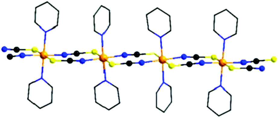 | ||
| Fig. 1 View of one chain in the crystal structures of compounds of the general composition [Co(NCX)2(L)2]n (X = S, Se; L = neutral N-donor co-ligand). For clarity, only the 6-membered rings of the different co-ligands are shown and the hydrogen atoms are omitted. | ||
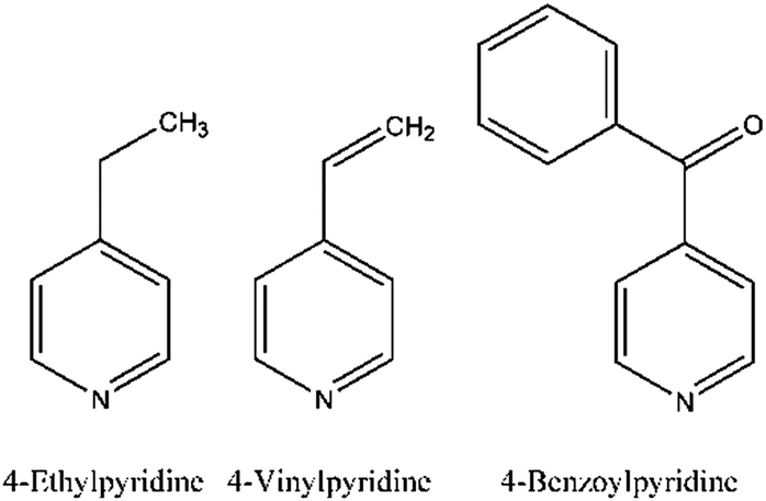
For the present study we chose 4-vinylpyridine (Scheme 1) which is topologically very similar to 4-ethylpyridine reported earlier and which differs only by two H atoms. In this case it would be of interest to find out which structure the vinylpyridine compound will adopt and what will be its magnetic ground state in comparison to 4-ethylpyridine. We also chose the larger 4-benzoylpyridine (Scheme 1) as co-ligand, for which longer inter-chain distances are expected but surprisingly a compound was obtained, in which the N and S atoms of the anionic ligands are cis-oriented, whereas the co-ligands are still trans to each other. This coordination is different from that observed in all other compounds of this family and allows us to study the influence of a slightly different metal coordination on the magnetic properties.
 | ||
| Scheme 1 | ||
It is noted that for these two co-ligands the crystal structures of compounds of composition Co(NCS)2(4-vinylpyridine)4 as well as Co(NCS)2(4-benzoylpyridine)4 were already reported, where the 4-vinylpyridine compound existed in two polymorphic modifications.58–60 These compounds consist of discrete complexes, in which the Co(II) cations are octahedrally coordinated by two terminal N-bonded thiocyanato anions and four N-coordinating co-ligands. Moreover, the crystal structure of a compound of composition Co(NCS)2(4-vinylpyridine)2 was also reported, that exactly corresponded to the composition expected for the desired chain compound. However, this compound consisted of discrete complexes in which the Co(II) cations were tetrahedrally coordinated by two terminal thiocyanato anions and two 4-vinylpyridine co-ligands.59
In this article the crystal structures of two new chain compounds are presented together with their magnetic characterization. The aim of this paper is detailed comparative studies of DC and AC magnetic properties and specific heat measurements as well as ab initio and DFT calculations of relevant magnetic parameters. Among others, we would also like to see if there is any influence of the cis vs. trans coordination of the Co cations on the magnetic properties.
Experimental section
Syntheses
4-Benzoylpyridine, 4-vinylpyridine and Co(NCS)2 were obtained from Alfa Aesar. All solvents were used without further purification.A crystalline powder on a larger scale was obtained by reacting Co(NCS)2 (175.1 mg, 1.00 mmol) and 4-vinylpyridine (215.7 μL, 2.00 mmol) in 2.0 mL of acetonitrile for 3 d. Elemental analysis: calcd (%) for C16H14CoN4S2: C 49.87, H 3.66, N 14.54, S 16.64; found C 48.42, H 3.68, N 14.55, S 16.64. IR (ATR, cm−1): νmax = 3069 (w), 2987 (w), 2893 (w), 2354 (w), 2320 (w), 2100 (s), 1610 (s), 1545 (m), 1503 (m), 1413 (m), 1223 (m), 1066 (w), 1014 (m), 987 (s), 934 (s), 934 (s), 798 (m), 642 (w), 566 (m).
X-Ray powder diffraction (XRPD)
The XRPD measurements were performed by using (1) a PANanalytical X'Pert Pro MPD Reflection Powder Diffraction System with CuKα radiation (λ = 154.0598 pm) equipped with a PIXcel semiconductor detector from PANanalytical and (2) a Stoe Transmission Powder Diffraction System (STADI P) with CuKα radiation that was equipped with a linear position-sensitive MYTHEN detector from STOE & CIE.IR spectroscopy
FT IR spectra were recorded on a Genesis series FTIR spectrometer, by ATI Mattson, in KBr pellets, as well as by using an Alpha IR spectrometer from Bruker equipped with a Platinum ATR QuickSnap™ sampling module between 375 and 4000 cm−1.Elemental analysis
CHNS analysis was performed using an EURO EA elemental analyzer, fabricated by EURO VECTOR Instruments and Software.Single-crystal structure analyses
Data collection was performed using an imaging plate diffraction system IPDS-2 (1 and 2) with Mo-Kα-radiation from STOE & CIE. The structure solutions were performed by direct methods using SHELXS-97 and structure refinements were performed against F2 using SHELXL-97. All non-hydrogen atoms were refined with anisotropic displacement parameters. The hydrogen atoms were positioned with idealized geometry and were refined isotropically with Uiso(H) = −1.2· Ueq(C) using a riding model. In 1 a part of the co-ligand is disordered and was refined using a split model. For 2 the absolute structure was determined and is in agreement with the selected setting (Flack x = 0.014(16) by classical fit to all intensities and 0.012(6) from 1487 selected quotients (Pearson's method)). Selected crystal data are shown in Table S1 (ESI†). CCDC 1507089 (1), and CCDC 1507085 (2) contain the supplementary crystallographic data for this paper.Magnetic measurements
Magnetic measurements were performed for polycrystalline samples using a Quantum Design MPMS XL magnetometer. In order to avoid reorientation of grains in a magnetic field the powders were mixed with Nujol and frozen below 250 K with zero field. Diamagnetic corrections of sample holders and the core diamagnetism were subtracted.Specific heat measurements
Specific heat was measured by the relaxation technique using the Quantum Design PPMS. Powders were pressed without any binder into a thin pellet. Apiezon N grease was used to ensure thermal contact of the samples with the microcalorimeter. The heat capacity of the calorimeter with the grease was measured before each run and subtracted subsequently.Computational details
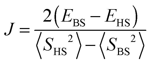
In the DFT calculations the positions of the non-hydrogen atoms have been taken from the crystal structures of 1 and 2, which we use as initial molecular structures for the different computational models (see Computational studies). The positions of all hydrogen atoms were optimized using the Turbomole 6.6 package of programs61 at the RI-DFT62–65/BP8666,67/def2-SVP68 level of theory. For these optimizations Co(II) ions have been replaced by diamagnetic Zn(II) ions to achieve a faster SCF convergence and to save computational time. In the case of 1 and 2 the magnetic coupling constants have been calculated within constrained DFT (CDFT)69,70 and broken-symmetry DFT (BS-DFT) approaches. In both cases the B3LYP hybrid functional66,71,72 in combination with def2-TZVPP (Co), def2-TZVP (S, N), and def2-SVP (remaining atoms) basis sets68 was used. CDFT calculations have been performed with NWChem 6.673 whereas Turbomole 6.6 was used for BS-DFT calculations. Within the CDFT calculations two spin constraints that contained the specific Co(II) ion and its six donor atoms were applied to perform the high-spin state (HS) and broken-symmetry (BS) state calculations. Subsequently, the magnetic coupling constant J was calculated by eqn (1) with SA = SB = 3/2 for a Heisenberg Hamiltonian .
.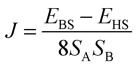 | (1) |
 | (2) |
Results and discussion
Synthetic aspects and crystal structures of compounds 1 and 2
The reaction of equimolar amounts of cobalt(thiocyanate) with 4-vinylpyridine, respectively 4-benzoylpyridine, leads to the formation of the two new compounds 1 and 2. If more co-ligand is used the known complexes Co(NCS)2(4-vinylpyridine)4 and Co(NCS)2(4-benzoylpyridine)4 are formed.58,60 IR spectroscopic investigations revealed the CN stretching vibration at values of 2100 cm−1 (1) and 2111 cm−1, respectively 2132 cm−1 (2), clearly indicating that in these compounds the Co(II) cations are linked by the anionic ligands (Fig. S2 and S3, ESI†). This is somehow surprising, because, as mentioned above, a compound of composition Co(NCS)2(4-vinylpyridine)2 was already reported to form discrete tetrahedral complexes, for which a value for the CN stretch of about 2050 cm−1 is expected.59 Therefore, it is highly likely that a different modification was obtained, using the synthesis from solution.[Co(NCS)2(4-vinylpyridine)2]n (1) crystallizes in the triclinic space group P![[1 with combining macron]](https://www.rsc.org/images/entities/char_0031_0304.gif) with 2 formula units in the unit cell. The asymmetric unit consists of two crystallographically independent Co(II) cations, which are located on centers of inversion, and two thiocyanato anions as well as two 4-vinylpyridine ligands in general positions (Fig. S4, ESI†). In the crystal structure, the Co cations are always trans-coordinated by the two N- and two S-bonding thiocyanato anions as well as two co-ligands and this is the usual coordination observed in this family of compounds. The Co–N bond lengths of 2.050(2) and 2.164(2) Å and the Co–S bond lengths of 2.5862(7) and 2.6051(7) Å are comparable to those in similar compounds (Table S1, ESI†). The Co(II) cations are linked into chains by pairs of thiocyanato anions via a μ-1,3-bridging coordination (Fig. 2, top).
with 2 formula units in the unit cell. The asymmetric unit consists of two crystallographically independent Co(II) cations, which are located on centers of inversion, and two thiocyanato anions as well as two 4-vinylpyridine ligands in general positions (Fig. S4, ESI†). In the crystal structure, the Co cations are always trans-coordinated by the two N- and two S-bonding thiocyanato anions as well as two co-ligands and this is the usual coordination observed in this family of compounds. The Co–N bond lengths of 2.050(2) and 2.164(2) Å and the Co–S bond lengths of 2.5862(7) and 2.6051(7) Å are comparable to those in similar compounds (Table S1, ESI†). The Co(II) cations are linked into chains by pairs of thiocyanato anions via a μ-1,3-bridging coordination (Fig. 2, top).
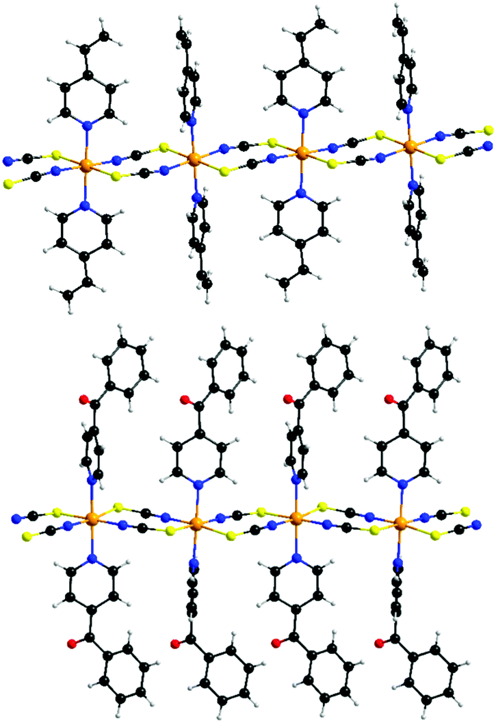 | ||
| Fig. 2 View of the cobalt thiocyanato chains in compound 1 (top) and 2 (bottom). An ORTEP plot of both compounds can be found in Fig. S4 and S5 in ESI.† | ||
The 4-benzoylpyridine compound 2 crystallizes in the orthorhombic space group P212121 with four formula units in the unit cell. The asymmetric unit consists of one Co cation, two thiocyanato anions and two 4-benzoylpyridine ligands (Fig. S5, ESI†). The Co cations are octahedrally coordinated by two N- and two S-bonding thiocyanato anions as well as two N-bonding co-ligands, with bond lengths and angles comparable to that in 1 (Table S3, ESI†). As in compound 1, the N-donor co-ligands are still trans-coordinated but for the anionic ligands a cis-coordination is found that was never observed before in this class of compounds. The Co(II) cations are linked by pairs of μ-1,3-bridging anionic ligands into linear chains (Fig. 2, bottom). The intra-chain distances between the Co centers amount to 5.653 Å in compound 1 and to 5.588 Å in compound 2 (Table 1). The longest inter-chain distance is observed for the 4-vinylpyridine compound, which is somehow surprising, because 4-benzoylpyridine is the larger ligand. However, this might be traced back to the different arrangement of the chains in the crystal (see below).
| Compound | Intra-chain/Å | Inter-chain/Å |
|---|---|---|
| 1 | 5.653 | 8.174 |
| 2 | 5.588 | 6.755 |
In 1 the N vectors of the co-ligands of neighboring chains are all parallel, which belongs to one of the two possible arrangements of chains in this family of compounds (Fig. S6, ESI†). It is noted that this arrangement is different from that in [Co(NCS)2(4-ethylpyridine)2]n, in which the N–N vectors are canted. This is somehow surprising, because as mentioned in the Introduction, both ligands are structurally very similar, and therefore, similar crystal structures are expected. However, the 4-benzoylpyridine compound adopts the arrangement in which the N–N vectors are canted (Fig. S6, ESI†).
Based on the structural data, the powder pattern for compounds 1 and 2 was calculated and compared with the experimental pattern, which shows that most compounds were obtained as pure crystalline phases (Fig. S7 and S8, ESI†).
Magnetic investigations – static properties
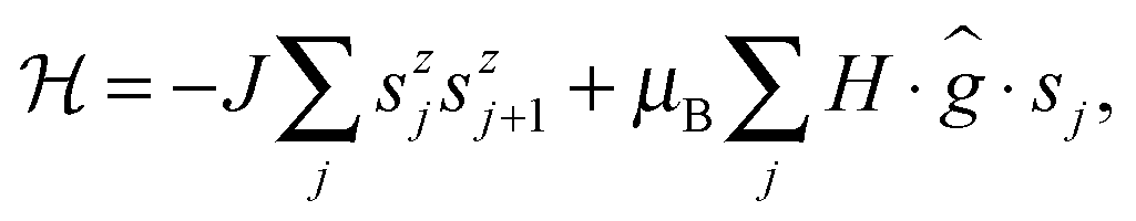
To get information about the magnetic ground state of 1 and 2, the magnetic susceptibility χ was measured as a function of temperature in a weak magnetic field of 100 Oe (Fig. 3, inset). The temperature dependence of the χT product is shown in the main part of Fig. 3 to illustrate the simultaneous action of the spin–orbit interaction of the Co(II) ion and of the dominant intra-chain magnetic interaction. They nearly compensate each other above 100 K, but below 50 K the χT product strongly increases, pointing that the dominant interaction is ferromagnetic.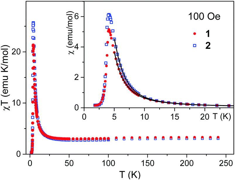 | ||
| Fig. 3 Temperature dependence of the χT product (main figure) and of the magnetic susceptibility χ (inset) measured in magnetic field of 100 Oe for 1 and 2. Solid lines are from fits (see text). | ||
To understand the low temperature magnetic behavior it should be taken into account that the Co(II) ion in an octahedral axially distorted coordination is well described with the effective spin s = 1/2 and a strongly anisotropic g factor. To estimate relevant magnetic parameters of the chain of Ising spins we used the Hamiltonian
 | (3) |
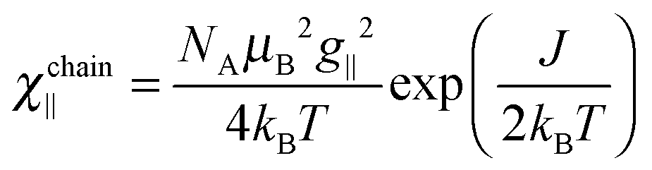 | (4) |
 | (5) |
 | (6) |
| χ = (χ∥ + 2χ⊥)/3. | (7) |
| Compound | 1 | 2 |
|---|---|---|
| T c (K) | 3.90(5) | 3.70(5) |
| J/kB (K) | 27(3) | 32(2) |
| g ∥ | 7.3(2) | 7.0(2) |
| g ⊥ | 0.0(1) | 0.0(1) |
| zJ′/kB (K) | −0.27(2) | −0.24(2) |
| a (emu mol−1) | 0.0098(7) | 0.0076(6) |
In this context it is noted that J values obtained directly from the slope of the ln(χT) vs. reciprocal temperature curve (Fig. S9, ESI†) are considerably lower than those obtained from the fit. The difference might originate from the antiferromagnetic inter-chain interaction or from deviation of 1 and 2 from assumptions of the Hamiltonian given in eqn (3).
Magnetization versus temperature was measured also in the zero-field cooled and field cooled (FC/ZFC) regime (Fig. 4). In low magnetic fields an antiferromagnetic maximum is observed but in higher fields a metamagnetic transition occurs. No bifurcations between ZFC and FC curves are observed for compound 1. For 2 small bifurcations are observed in the field range up to 500 Oe. These bifurcations are hardly seen in the scale of Fig. 4 but they are better visible in the χ vs. T presentation (Fig. S10, ESI†).
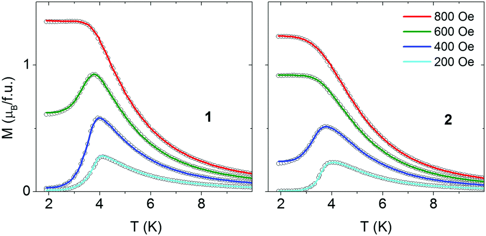 | ||
| Fig. 4 Temperature dependence of magnetization recorded for 1 (left) and 2 (right) in various magnetic fields following zero-field cooling (open points) and field cooling (lines). | ||
Field dependent magnetization curves, measured at 1.8 K in the high field range, are shown in Fig. 5. No saturation is observed even at high fields, which is in accordance with the high magnetic anisotropy of Co(II) ions. The magnetization at high fields is slightly higher for 1 than for 2, which may originate from the different coordination of Co(II) in both compounds.
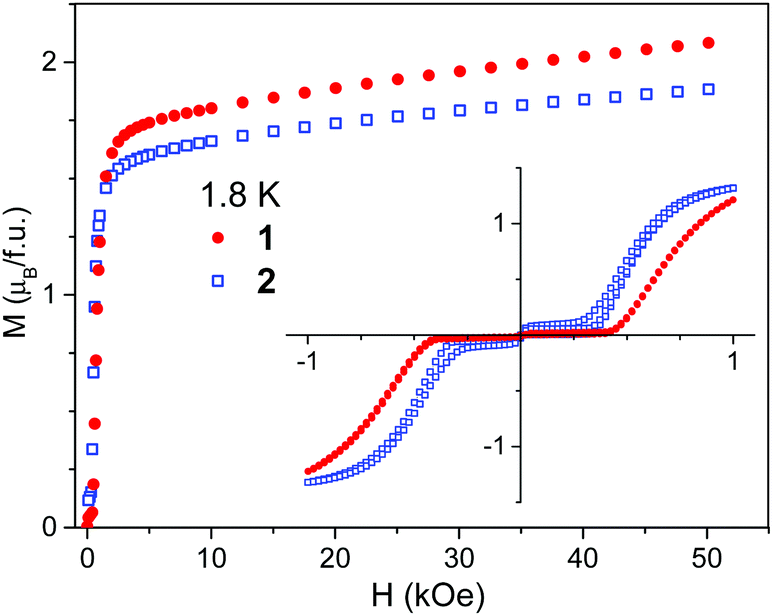 | ||
| Fig. 5 Field dependent magnetization measured at 1.8 K for compounds 1 and 2. Inset shows magnetic hysteresis loops registered in the low field range. | ||
The field dependent magnetization was also separately measured in weak fields. The experimental data collected at 1.8 K are presented in the inset of Fig. 5. They were recorded in the field cycling between −1 and +1 kOe. Data collected at higher temperatures can be found in Fig. S11–S13 in ESI.† It is seen that below Tc a magnetization jump occurs. This jump observed in the field Hc of ∼450 Oe for 1 and ∼350 Oe for 2 at 1.8 K is a sign of metamagnetic transition. No hysteresis loop is observed for 1 down to 1.8 K. For 2 a narrow hysteresis loop is observed in the field range 250–500 Oe and a second small jump near 0 Oe, the origin of which is not clear to us (Fig. S14, ESI†).
M(H) plots made in the field range 0–1000 Oe for 1 and 2 at various temperatures (Fig. S12 and S13, ESI†) were used to construct the phase diagrams (Fig. 6). However, points below 150 Oe in these diagrams were determined as the maximum of d(χT)/dT to reach an agreement with the specific heat study (Fig. S15, ESI†; see below). The relation between d(χT)/dT and magnetic specific heat was derived by Fisher for simple antiferromagnets85 but also tested for a variety of antiferromagnets.86
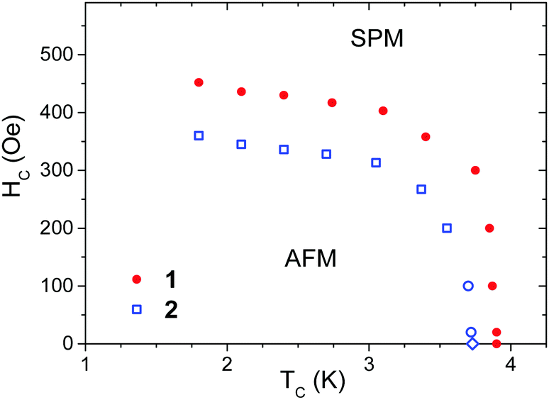 | ||
| Fig. 6 Magnetic phase diagram of 1 (solid dots) and 2 (open squares) with antiferromagnetic (AFM) and saturated paramagnetic (SPM) phases. | ||
Specific heat measurements
To confirm the long range magnetic ordering in compounds 1 and 2, specific heat (C) measurements were performed (Fig. 7). The temperature dependence of C measured at different applied fields is shown in Fig. S16 and S17 (ESI†). A distinct peak of C(T) is present at 3.80 K for 1, and at 3.68 K for 2, which marks the onset of the second order magnetic ordering transition, in good agreement with the results of magnetic measurements.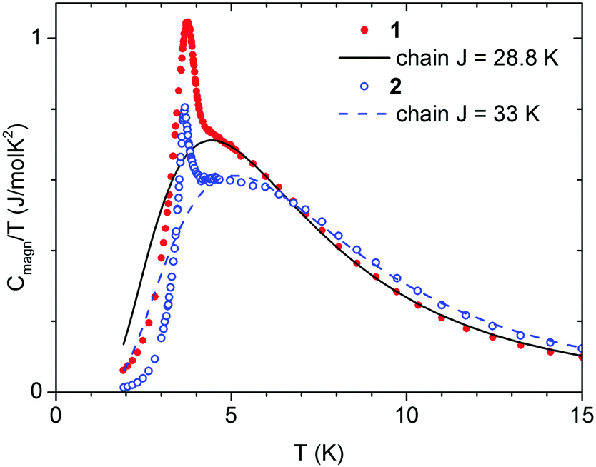 | ||
| Fig. 7 Magnetic contribution Cmagn of the specific heat, obtained for compounds 1 and 2, shown as C/T. The lines denote the fitted contribution related to the exchange interaction J within chains of Ising spins. | ||
The field of 0.4 kOe shifts the peak for 1 to a bit lower temperature, 3.75 K, which is typical for an antiferromagnetic structure. For 2 the field of 0.4 kOe is already above the critical field (see Fig. 6) and the C(T) peak is completely reduced. The observed peaks of specific heat are on the background that originates from the crystal lattice vibrations, but also from magnetic exchange interaction within chains of Co(II) ion spins. To calculate the lattice contribution we used the linear combination of the Debye and Einstein models of the phonon density of states to account for both acoustic and optical phonon bands.
Below 40 K it was enough to assume a single acoustic branch described by θD and a single optical branch described by θE, producing together
| Clattice = ADCDebye(T,θD) + AECEinstein(T,θE) | (8) |
Cchain = NAkB(J/4kBT)2![[thin space (1/6-em)]](https://www.rsc.org/images/entities/char_2009.gif) sech2(J/4kBT) sech2(J/4kBT) | (9) |
This model, however, does not contain inter-chain interaction, and cannot explain long range ordering. For this reason, the sum Clattice + Cchain was fitted to C/T data in the range from 4.5 to 40 K, i.e. only above the critical temperature. For 1 we obtained θD = 77.2(5) K, θE = 148.5(1.8) K, AD = 1.88(3), AE = 4.36(7) J (mol K)−1, and J/kB = 28.8(4) K. For 2 we obtained θD = 79.8(0.6) K, θE = 149(2) K, AD = 2.46(4), AE = 4.96(7) J (mol K)−1, and J/kB = 33.2(4) K. The Clattice and Cchain curves, calculated using these parameters, are drawn in Fig. S18 and S19 (ESI†). The magnetic contribution to specific heat, obtained by subtracting Cmagn = C − Clattice, is shown in Fig. 7. The entropy change, calculated by integrating Cmagn/T in the range from 2 to 40 K, is 5.53 for 1 and 5.37 J (mol K)−1 for 2, which is close to the expected NAkBln2 = 5.76 J (mol K)−1. Only a fraction of this entropy change is below Tc (0.69 and 0.34 J (mol K)−1, respectively). Such behavior is characteristic for quasi-one dimensional systems.87 Most importantly, the J values obtained from the analysis of calorimetric measurements agree very well with the J values obtained from the analysis of magnetic measurements.
Dynamic magnetic properties
Fig. 8 presents the temperature dependence of the AC magnetic susceptibility of 1 and 2 measured at various frequencies and zero DC field. In Fig. S20 (ESI†) also the data collected in field close to Hc are shown. As seen, in zero DC field the frequency dispersion occurs in the temperature range much below Tc but in field close to Hc this temperature range is considerably extended and the maximum value of χ considerably increases, especially for 2. In addition, for 2 the maximum of χ′′ at first increases with increasing temperature and then decreases.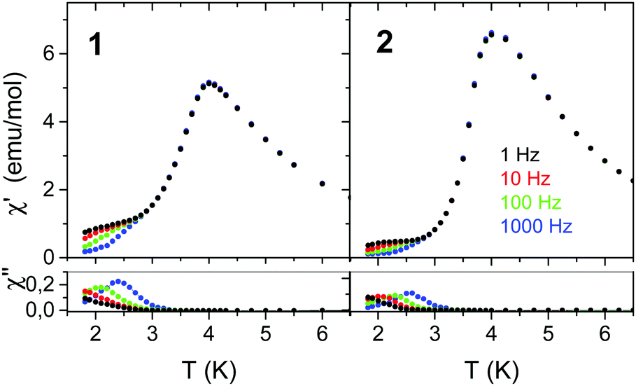 | ||
| Fig. 8 Temperature dependence of χAC registered at various frequencies for 1 and 2 in zero DC field. | ||
The Mydosh parameter ϕ = ΔTm/[TmΔ(logf)] in zero DC field determined from the temperature shift of χ′′ is ϕ ≈ 0.15 for 1 and ϕ ≈ 0.10 for 2, which is in the range expected for superparamagnets and single chain magnets.88
The frequency behavior of χAC observed for compounds 1 and 2 at various temperatures in zero field is presented in Fig. 9. For analysis the generalized Debye formula was used, which written for a single distribution of relaxation times has the following form:
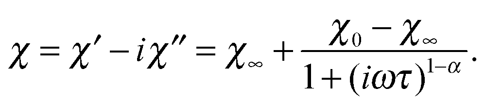 | (10) |
 | ||
| Fig. 9 Frequency dependent AC susceptibility for 2 (left) and 1 (right) in HDC = 0 Oe. Solid lines are fits of the generalized Debye relaxation model. | ||
The data of zero field for 1 and 2 could be well fitted with a single distribution. A small contribution of a second distribution observed for 1 at the lowest temperatures and lowest frequencies (see also the Cole–Cole plot; Fig. S21 and S22, ESI†) was omitted in the analysis. For both compounds the α parameter is relatively small (∼0.2) at the upper temperature limit but increases with decreasing temperature, becoming ∼0.55 at the lower temperature limit of 1.8 K (Tables S4 and S5, ESI†). The corresponding data in field could be successfully fitted only for 1 assuming one distribution (the data for 2 were more complex and could not be fitted). The values of α determined for 1 in field were 0.45–0.54 in the corresponding temperature range 1.8–3.0 K. It is worth to note the higher value of α at the upper temperature limit in relation to zero field.
The values of relaxation times for 1 and 2 obtained from fits are plotted as lnτ vs. 1/T dependence in Fig. 10 and fitted using the Arrhenius equation
| τ = τ0exp(ΔE/kBT), | (11) |
 | ||
| Fig. 10 Temperature dependence of the relaxation time τ determined at Hdc = 0 Oe for 1 and 2 and at Hdc = 600 Oe for 1. Straight lines were fitted using the Arrhenius equation. | ||
As seen in Fig. 10, the straight line dependence in the whole temperature range used (red lines) was obtained for 1 in both zero DC field and 600 Oe DC field. The following values of parameters for zero DC field were obtained from the plot: ΔE/kB = 36.5 ± 2 K, τ0 = (1.77 ± 0.50) × 10−11 s. The corresponding values for 600 Oe field were as follows: ΔE/kB = 42.8 ± 2 K, τ0 = (1.76 ± 0.45) × 10−10 s. It is noted that the value of τ0 increased in field by one order of magnitude, which is in agreement with ref. 89.
For 2 two straight line intervals were obtained for Hdc = 0 Oe with the crossover temperature T* ∼ 2.2 K. Such intervals are usually interpreted as the finite chain regime (at lower temperatures; denoted below with subscript k = 1) and the infinite chain regime (at higher temperatures; k = 2). Thus, for 2, τ01 = 2.4 × 10⁻¹⁰ s, ΔE1/kB = 35.5(1.0) K and τ02 = 1.4 × 10⁻¹³ s, ΔE2/kB = 51.9(2.6) K. It is noted that the value ΔE1 is close to the value 36.5 K of 1. The corresponding parameters for 400 Oe field, as already mentioned above, could not be reliably determined.
The crossover from k = 1 to k = 2 observed for 2 at T* can be used to estimate the chain length n through the relation 2n exp(−2Js2/kBT*) = 1, assuming the same length of all chains.16 For J = 32 K and T* = 2.2 K the chains are fairly long with n ∼ 700 links.
Discussion of the magnetic properties
According to Coulon et al.16 ΔE for anisotropic Heisenberg systems ΔEk may be written as composed of the following two terms:| ΔEk = kΔξ + ΔA, | (12) |
Initially, after the discovery of SCM, it was believed that slow relaxations may be observed only in systems with weakly interacting chains, so weakly that no magnetic ordering occurs or it occurs at very low temperature. Soon, it was demonstrated by Coulon et al.89 that slow relaxations can also exist in the antiferromagnetic (AF) phase and that the relaxation time is enhanced in DC magnetic field being maximum close to the antiferromagnetic–paramagnetic phase transition. Later on, slow relaxations in the AF phase were also reported by Miyasaka et al., who observed them below the blocking temperature TB ∼ 5 K, significantly lower than the Néel temperature TN = 9.4 K. The hysteresis loops in the AF phase, which were presented in both referenced articles, appeared due to slow relaxations of SCM. Obviously, slow relaxations in the AF phase should disappear with the increase of the interchain interactions or more precisely with the increase of the zJ′/J ratio and this increase should be associated with the decrease of the TB/TN ratio. This remark refers also to other AF compounds Co(NCS)2L2 previously studied.41–45 All are close to the disappearance of SCMs due to significant interchain interactions.
On the other hand, all these compounds show strong relaxations in magnetic fields close to Hc. We have shown that relaxations observed for 1 in 600 Oe can be described with the generalized Debye model and a single but rather broad distribution of the relaxation times (α ∼ 0.5). The more complex relaxational behavior of 2 in field (see Fig. S20, ESI†) may be related to the chosen applied field value because, as known from the previous studies, in fields above Hc the material is in the mixed phase between antiferromagnetic and paramagnetic phases. Then the 3D ferromagnetically ordered domains or fractal spin glass clusters form.91 Also the observed crossover as well as the more complex crystal structure having two directions of Npyr–Co–Npyr vectors (Npyr is the nitrogen atom of pyridine) may influence the relaxational behavior of 2.
It is noted that in 1 and 2 as well as in other compounds of the Co(NCS)2L2 family the only possible interchain interactions are dipolar interactions. Sometimes they lead to AF, and sometimes to FM interactions. For a better understanding of the magnetic properties of this family the knowledge of the easy direction of anisotropy is necessary.
We do not see a clear difference in magnetic properties between trans and cis coordination of Co-ions in 1 and 2. The eventual difference is so small that it is obscured by the difference in crystal structures and large distortion of the coordination octahedron.
Computational studies
Our results with the CDFT calculations show that employing constraints to restrict the spin densities on the Co(II) centers and their first coordination sphere allows the use of dinuclear model systems to qualitatively reproduce the magnetic coupling in 1 and 2. To gain further insight, we performed calculations for which the sodium ions were replaced by simple point charges located at the positions of the metal ions. In contradiction to the experiment this leads to an antiferromagnetic ground state in the case of 1 (J = −41.3 K) and a weak ferromagnetic coupling in the case of 2 (J = 12.7 K). Thus, we conclude that a reasonable chemical representation of the metal centers at the terminal positions of the model fragment is required to reproduce the experimental results, which cannot be achieved by simple point charges. To further probe the possible reduction of the computational model we also tested to substitute the apical pyridine-based co-ligands by an unsubstituted pyridine. For both cases this results in the prediction of a rather strong antiferromagnetic coupling (1: J = −108.1 K, 2: J = −86.9 K). This clearly indicates that also the electronic properties of the apical co-ligands might play a crucial role.
As a result, CDFT calculations on the sodium terminated dinuclear model system are suitable to describe the intra-chain interactions in compounds 1 and 2. These calculations are in agreement with the observed small differences in magnetic coupling as the two configurations at the cobalt centers are concerned (1: trans- and 2cis-position).
In general, high-spin Co(II) ions in an octahedral geometry possess a 4T1g ground state which is primarily responsible for their magnetic properties due to considerable energy gaps to higher quartet (4T2g, 4A2g) and doublet states (2G, 2P, etc.). Nevertheless, the higher energetic states have a slight influence on the electronic ground state, and thus have to be taken into account. Table S7 (ESI†) lists the corresponding CASSCF and CASPT2 energies for all quartet and the 12 lowest doublet states of 1-Co1, 1-Co2, and 2. As it can be seen the high-spin 4F multiplet with its 4T1g, 4T2g, and 4A2g subterms is the ground state in all cases independent of whether dynamic correlation is excluded (CASSCF) or included (CASPT2). Nevertheless, dynamic correlation is essential to reasonably describe the doublet states as it can be seen by the significant changes in their relative energies upon inclusion. For CASPT2 the lowest doublet states are well separated from the lowest quartet state with energy gaps of 9173, 9030, and 9791 cm−1 for 1-Co1, 1-Co2, and 2, respectively. However, the description of these individual states is not sufficient to get an accurate insight into the magnetic properties due to the lack of state-mixing and spin–orbit coupling.
RASSI-SO/SINGLE_ANISO calculations on the basis of the CASPT2 wave functions have been performed to adequately describe the energetic states. This leads to 6 doubly degenerated spin–orbit coupled states (J = 1/2, 3/2, and 5/2), denoted as Kramers doublets (KDs), with predominant contribution from the 4T1g subterm of the 4F multiplet. However, even at room temperature only the lowest two KDs are expected to be thermally populated, due to the relative energies of the higher KD states (see Table S8, ESI†). The alternating orientation of the 4-vinylpyridine co-ligands in the case of 1 has a slight influence on the calculated energy gap between the ground and the first excited KD. The parallel arrangement of 4-vinylpyridine with respect to the chain orientation (1-Co2) leads to a slightly higher energy gap of 192 cm−1 as compared to the perpendicular case (1-Co1) with 183 cm−1. On the other hand, for compound 2 both parallel and perpendicular orientations of the 4-benzoylpyridine co-ligand are observed at a single Co(II) ion which in this case is associated with a significantly higher first excited KD at 270 cm−1. However, this effect cannot be attributed to a single structural parameter, due to the additional differences in the (NCS)4 coordination environment at the Co(II) centers (1: cis, 2: trans) as well as differences in the structural and electronic properties imposed by the substituents at the co-ligands.
Calculated zero-field splitting (ZFS) parameters and g values for an effective spin of Seff = 3/2 are summarized in Table 3 and show for both compounds the presence of an easy-axis anisotropy. In accordance with the above-mentioned results a larger absolute axial ZFS parameter D is obtained for 2 (−124.99 cm−1) as compared to 1-Co1 (−85.87 cm−1) and 1-Co2 (−83.24 cm−1). Additionally, in all cases a significant rhombic distortion in terms of large absolute E values can be observed (1-Co1: −18.54 cm−1; 1-Co2: −27.67 cm−1; 2: −29.69 cm−1) leading to remarkable E/D ratios.
| 1-Co1 | 1-Co2 | 2 | |
|---|---|---|---|
| D/cm−1 | −85.87 | −83.24 | −124.99 |
| E/cm−1 | −18.54 | −27.67 | −29.69 |
| E/D | 0.22 | 0.33 | 0.24 |
| g x | 1.971 | 1.885 | 1.683 |
| g y | 2.233 | 2.365 | 1.823 |
| g z | 2.980 | 2.974 | 3.291 |
The corresponding anisotropy axes are depicted in Fig. 11. In all cases a nearly parallel alignment of the main anisotropy axis with the N–N vector of the two apical pyridine-based co-ligands can be found. The angle between the N–N vector and the main anisotropy axis is found to be 2.5, 2.8, and 0.3° for 1-Co1, 1-Co2, and 2, respectively. In both compounds the corresponding hard plane of magnetization is formed within the S2N2 coordination plane of the four NCS ligands (angles between the hard plane and the S2N2 coordination plane: 1-Co1: 2.4°, 1-Co2: 3.1°, 2: 1.6°). The basic orientation of the two hard-axes approximately along the Co–N and Co–S bonds can explain the noticeable rhombic ZFS parameter E due to a different electronic structure of these N and S donor atoms.
 | ||
| Fig. 11 Ab initio calculated (Seff = 3/2) anisotropy axes (blue dashed lines: easy-axes; red dashed lines: hard-axes) of 1-Co1, 1-Co2, and 2 projected onto dinuclear Co(II) fragments of 1 (top) and 2 (bottom). The angle between the two easy-axes of 1-Co1 and 1-Co2 is 9.0°. In the respective top view on the right hand side the hydrogen atoms as well as pyridine-based co-ligands are omitted for clarity. | ||
The calculated g values (Seff = 3/2) given in Table 4 show in accordance with the ZFS an easy-axis anisotropy (gz > gx, gy) with gz values of 2.980, 2.974, and 3.291 for 1-Co1, 1-Co2, and 2, respectively. The large gz values as compared to (pseudo)-tetrahedrally coordinated Co(II) complexes95 are the result of a strong spin–orbit contribution which is most pronounced in the case of 2. It is interesting to note that this goes along with the smallest deviation from an ideal octahedral coordination sphere in the case of 2 as obtained by continuous shape measures (S(Oh) for 1-Co1: 1.057, 1-Co2: 1.130, and 2: 0.865).96,97
| KD | 1-Co1 | 1-Co2 | 2 | |
|---|---|---|---|---|
| 1 | E KD/cm−1 | 0 | 0 | 0 |
| g x | 1.198 | 1.532 | 1.397 | |
| g y | 1.484 | 2.300 | 1.486 | |
| g z | 8.445 | 7.997 | 8.747 | |
| 2 | E KD/cm−1 | 183 | 192 | 270 |
| g x | 2.905 | 2.432 | 0.424 | |
| g y | 2.975 | 2.507 | 1.807 | |
| g z | 4.840 | 4.938 | 4.194 |
The calculated g tensor components for the two lowest KDs within an effective spin formalism of Seff = 1/2 are listed in Table 4. For both compounds 1 and 2 the ground state KD possesses an easy-axis anisotropy which is in agreement with the previous results (for Seff = 3/2). Fig. S27 (ESI†) shows the corresponding ground state magnetic axes for 1 and 2. The calculated ground state gz values (1-Co1: 8.445, 1-Co2: 7.997, 2: 8.747) are slightly overestimated as compared to the experimental data (1: 7.3(2), 2: 7.0(2)).
Noteworthily, the perpendicular arrangement of 4-vinylpyridine with respect to the chain orientation (1-Co1) leads to a slightly higher gz value as compared to the parallel case (1-Co2). The first excited KD in 1 and 2 also shows easy-axis anisotropy, but with smaller gz values and larger transversal components gx and gy. The corresponding principal axes for the first excited KD are depicted in Fig. S28 (ESI†). For compound 2 the orientation of the principal axes is similar to what was observed for the ground state, whereas this is surprisingly not the case for the Co(II) centers of 1-Co1 and 1-Co2. For the latter cases the easy-axes of the first excited state are within the S2N2 coordination plane and oriented perpendicular to the corresponding plane of the aromatic ring system of the 4-vinylpyridine co-ligands.
There is an obvious discrepancy between experimentally estimated effective barriers and the calculated single-ion barriers in terms of their first excited KD energies. Thus, the presence of dominant relaxation processes other than the thermal Orbach process can be assumed. Concerning quantum tunneling within a single Co(II) ion fragment Fig. S29 and S30 (ESI†) show the average dipole transition matrix elements for the first two KDs of 1 and 2. Obviously, for all model systems a considerable quantum tunneling of magnetization would be expected due to the large dipole transition matrix elements within the ground state KD (1-Co1: 0.447; 1-Co2: 0.639; 2: 0.480). In contrast to 2, the first excited KD of 1-Co1 and 1-Co2 shows no large ![[small mu, Greek, macron]](https://www.rsc.org/images/entities/i_char_e0cd.gif) z value due to the change of the easy-axis orientation. Recently, a similar discrepancy (Ucalc = 264 cm−1 and Ueff = 25 cm−1) has been reported for a mononuclear octahedral Co(II) compound ([Co(H2O)2(CH3COO)2(py)2]) with two apical pyridine ligands for which a two-phonon Raman process was proposed.98 Moreover, it should be noted that 1 and 2 are not single-ion complexes but represent more complex magnetically coupled systems. Nevertheless, the performed single-ion ab initio calculations help to evaluate the axial anisotropy which revealed a slightly higher axial anisotropy in the case of 2 which goes together with a stronger intra-chain magnetic coupling. Due to the identical NCS-bridged equatorial coordination chains the axial anisotropy can be directly tuned by the apical co-ligands with their electronic influences.
z value due to the change of the easy-axis orientation. Recently, a similar discrepancy (Ucalc = 264 cm−1 and Ueff = 25 cm−1) has been reported for a mononuclear octahedral Co(II) compound ([Co(H2O)2(CH3COO)2(py)2]) with two apical pyridine ligands for which a two-phonon Raman process was proposed.98 Moreover, it should be noted that 1 and 2 are not single-ion complexes but represent more complex magnetically coupled systems. Nevertheless, the performed single-ion ab initio calculations help to evaluate the axial anisotropy which revealed a slightly higher axial anisotropy in the case of 2 which goes together with a stronger intra-chain magnetic coupling. Due to the identical NCS-bridged equatorial coordination chains the axial anisotropy can be directly tuned by the apical co-ligands with their electronic influences.
Conclusions
The major goal of this work consists of investigations of the influence of metal coordination and the crystal structure on the magnetic properties of 1D Co-thiocyanato coordination polymers. Therefore, two new compounds of the general formula [Co(NCS)2L2]n were synthesized (L is 4-vinylpyridine (1) or 4-benzoyl pyridine (2)). They are built up of ferromagnetic chains, which are weakly antiferromagnetically coupled, so they show magnetic ordering and a metamagnetic transition. While 1 shows a trans configuration of the anionic ligands along the exchange path, the configuration is different (cis) for 2. This different configuration results in slightly greater magnetic exchange for 2. Both compounds show single-chain magnet relaxations in the antiferromagnetic state. The intra-chain magnetic coupling obtained by CDFT calculations utilizing the corresponding dinuclear Co(II) fragments of 1 and 2 as models is in agreement with the experimental results. Ab initio calculations revealed the ground state easy-axis anisotropy in all cases with the easy-axis of magnetization aligned along the N–N vector of the pyridine-based apical ligands. Moreover, the calculations reveal the presence of significant rhombic ZFS as evidenced by large E values. The single-ion calculations clearly show that structural and electronic properties of the apical co-ligands influence the magnetic properties, e.g. in terms of the gz values. However, in 1 the alternating arrangement of the 4-vinylpyridine co-ligands (parallel and perpendicular) with respect to the chain orientation leads to a compensation of the higher magnetic anisotropy in the perpendicular arrangement (1-Co1). Therefore, further studies are planned to determine experimentally the easy direction of magnetic anisotropy and clarify the role of dipolar interactions leading to magnetic ordering, which is necessary to fully understand the variety of magnetic properties for this family of compounds.Acknowledgements
This project was supported by the Deutsche Forschungsgemeinschaft (Project No. NA 720/5-1) and the State of Schleswig-Holstein. We thank Professor Dr Wolfgang Bensch for access to his experimental facility. ZT thanks National Science Centre Poland for financial support granted under decision DEC-2013/11/B/ST3/03799. The research was in part carried out with the equipment purchased with the support of European Regional Development Fund within the Polish Innovation Economy Operational Program (POIG.02.01.00-12-023/08).References
- K. Liu, W. Shi and P. Cheng, Coord. Chem. Rev., 2015, 289–290, 74–122 CrossRef CAS.
- A. Caneschi, D. Gatteschi and F. Totti, Coord. Chem. Rev., 2015, 289–290, 357–378 CrossRef CAS.
- M. Atanasov, D. Aravena, E. Suturina, E. Bill, D. Maganas and F. Neese, Coord. Chem. Rev., 2015, 289–290, 177–214 CrossRef CAS.
- Y. Z. Zheng, G. J. Zhou, Z. Zheng and R. E. P. Winpenny, Chem. Soc. Rev., 2014, 43, 1462–1475 RSC.
- J. M. Clemente-Juan, E. Coronado and A. Gaita-Arino, Chem. Soc. Rev., 2012, 41, 7464–7478 RSC.
- D.-F. Weng, Z.-M. Wang and S. Gao, Chem. Soc. Rev., 2011, 40, 3157–3181 RSC.
- X. Y. Wang, C. Avendano and K. R. Dunbar, Chem. Soc. Rev., 2011, 40, 3213–3238 RSC.
- C. Train, M. Gruselle and M. Verdaguer, Chem. Soc. Rev., 2011, 40, 3297–3312 RSC.
- D. R. Talham and M. W. Meisel, Chem. Soc. Rev., 2011, 40, 3356–3365 RSC.
- S. Sanvito, Chem. Soc. Rev., 2011, 40, 3336–3355 RSC.
- J. S. Miller and D. Gatteschi, Chem. Soc. Rev., 2011, 40, 3065–3066 RSC.
- J. S. Miller, Chem. Soc. Rev., 2011, 40, 3266–3296 RSC.
- J. Mroziński, Coord. Chem. Rev., 2005, 249, 2534–2548 CrossRef.
- C. Coulon, V. Pianet, M. Urdampilleta and R. Clérac, in Molecular Nanomagnets and Related Phenomena, ed. S. Gao, Springer, Berlin Heidelberg, 2015, ch. 154, vol. 164, pp. 143–184 Search PubMed.
- S. Dhers, H. L. C. Feltham and S. Brooker, Coord. Chem. Rev., 2015, 296, 24–44 CrossRef CAS.
- C. Coulon, H. Miyasaka and R. Clérac, Struct. Bonding, 2006, 122, 163–206 CrossRef CAS.
- H. Miyasaka and R. Clérac, Bull. Chem. Soc. Jpn., 2005, 78, 1725–1748 CrossRef CAS.
- L. Bogani, A. Vindigni, R. Sessoli and D. Gatteschi, J. Mater. Chem., 2008, 18, 4733–4880 RSC.
- W.-X. Zhang, R. Ishikawa, B. Breedlovea and M. Yamashita, RSC Adv., 2013, 3, 3772–3798 RSC.
- H.-L. Sun, Z.-M. Wang and S. Gao, Coord. Chem. Rev., 2010, 254, 1081–1100 CrossRef CAS.
- R. Lescouëzec, L. M. Toma, J. Vaissermann, M. Verdaguer, F. S. Delgado, C. Ruiz-Pérez, F. Lloret and M. Julve, Coord. Chem. Rev., 2005, 249, 2691–2729 CrossRef.
- G. Bhargavi, M. V. Rajasekharan, J. P. Costes and J. P. Tuchagues, Dalton Trans., 2013, 42, 8113–8123 RSC.
- D.-P. Dong, Y.-J. Zhang, H. Zheng, P.-F. Zhuang, L. Zhao, Y. Xu, J. Hu, T. Liu and C.-Y. Duan, Dalton Trans., 2013, 42, 7693–7698 RSC.
- P. Hu, C. Zhang, Y. Gao, Y. Li, Y. Ma, L. Li and D. Liao, Inorg. Chim. Acta, 2013, 398, 136–140 CrossRef CAS.
- X.-B. Li, G.-M. Zhuang, X. Wang, K. Wang and E.-Q. Gao, Chem. Commun., 2013, 49, 1814–1816 RSC.
- K. S. Lim and C. S. Hong, Dalton Trans., 2013, 42, 14941–14950 RSC.
- T. Liu, H. Zheng, S. Kang, Y. Shiota, S. Hayami, M. Mito, O. Sato, K. Yoshizawa, S. Kanegawa and C. Duan, Nat. Commun., 2013, 4, 1–7 Search PubMed.
- V. Tangoulis, M. Lalia-Kantouri, M. Gdaniec, C. Papadopoulos, V. Miletic and A. Czapik, Inorg. Chem., 2013, 52, 6559–6569 CrossRef CAS PubMed.
- D.-F. Weng, B.-W. Wang, Z.-M. Wang and S. Gao, Coord. Chem. Rev., 2013, 257, 2484–2490 CrossRef CAS.
- M.-X. Yao, Q. Zheng, K. Qian, Y. Song, S. Gao and J.-L. Zuo, Chem. – Eur. J., 2013, 19, 294–303 CrossRef CAS PubMed.
- X. Chen, S.-Q. Wu, A.-L. Cui and H.-Z. Kou, Chem. Commun., 2014, 50, 2120–2122 RSC.
- V. Mougel, L. Chatelain, J. Hermle, R. Caciuffo, E. Colineau, F. Tuna, N. Magnani, A. de Geyer, J. Pécaut and M. Mazzanti, Angew. Chem., 2014, 126, 838–842 CrossRef.
- E. V. Peresypkina, A. M. Majcher, M. Rams and K. E. Vostrikova, Chem. Commun., 2014, 50, 7150–7153 RSC.
- J. Ru, F. Gao, T. Wu, M.-X. Yao, Y.-Z. Li and J.-L. Zuo, Dalton Trans., 2014, 43, 933–936 RSC.
- H. Miyasaka, T. Madanbashi, A. Saitoh, N. Motokawa, R. Ishikawa, M. Yamashita, S. Bahr, W. Wernsdorfer and R. Clérac, Chem. – Eur. J., 2012, 18, 3942–3954 CrossRef CAS PubMed.
- I. Bhowmick, E. A. Hillard, P. Dechambenoit, C. Coulon, T. D. Harris and R. Clerac, Chem. Commun., 2012, 48, 9717–9719 RSC.
- Z. Tomkowicz, M. Rams, M. Bałanda, S. Foro, H. Nojiri, Y. Krupskaya, V. Kataev, B. Büchner, S. K. Nayak, J. V. Yakhmi and W. Haase, Inorg. Chem., 2012, 51, 9983–9994 CrossRef CAS PubMed.
- R. Lescouëzec, J. Vaissermann, C. Ruiz-Pérez, F. Lloret, R. Carrasco, M. Julve, M. Verdaguer, Y. Dromzee, D. Gatteschi and W. Wernsdorfer, Angew. Chem., 2003, 115, 1521–1524 CrossRef.
- H. Miyasaka, M. Julve, M. Yamashita and R. Clérac, Inorg. Chem., 2009, 48, 3420–3437 CrossRef CAS PubMed.
- Y.-Z. Zhang, H.-H. Zhao, E. Funck and K. R. Dunbar, Angew. Chem., Int. Ed., 2015, 54, 5583–5587 CrossRef CAS PubMed.
- S. Wöhlert, J. Boeckmann, M. Wriedt and C. Näther, Angew. Chem., Int. Ed., 2011, 50, 6920–6923 CrossRef PubMed.
- J. Werner, Z. Tomkowicz, M. Rams, S. G. Ebbinghaus, T. Neumann and C. Näther, Dalton Trans., 2015, 44, 14149–14158 RSC.
- S. Wöhlert, Z. Tomkowicz, M. Rams, S. G. Ebbinghaus, L. Fink, M. U. Schmidt and C. Näther, Inorg. Chem., 2014, 53, 8298–8310 CrossRef PubMed.
- S. Wöhlert, T. Fic, Z. Tomkowicz, S. G. Ebbinghaus, M. Rams, W. Haase and C. Näther, Inorg. Chem., 2013, 52, 12947–12957 CrossRef PubMed.
- S. Wöhlert, U. Ruschewitz and C. Näther, Cryst. Growth Des., 2012, 12, 2715–2718 Search PubMed.
- J. Werner, M. Rams, Z. Tomkowicz, T. Runčevski, R. E. Dinnebier, S. Suckert and C. Näther, Inorg. Chem., 2015, 54, 2893–2901 CrossRef CAS PubMed.
- J. Werner, M. Rams, Z. Tomkowicz and C. Näther, Dalton Trans., 2014, 43, 17333–17342 RSC.
- S. Wöhlert, M. Wriedt, T. Fic, Z. Tomkowicz, W. Haase and C. Näther, Inorg. Chem., 2013, 52, 1061–1068 CrossRef PubMed.
- J. Boeckmann, M. Wriedt and C. Näther, Chem. – Eur. J., 2012, 18, 5284–5289 CrossRef CAS PubMed.
- S. Wöhlert, T. Runčevski, R. E. Dinnebier, S. G. Ebbinghaus and C. Näther, Cryst. Growth Des., 2014, 14, 1902–1913 Search PubMed.
- J. Werner, T. Runčevski, R. Dinnebier, S. G. Ebbinghaus, S. Suckert and C. Näther, Eur. J. Inorg. Chem., 2015, 3236–3245 CrossRef CAS.
- C. Näther, S. Wöhlert, J. Boeckmann, M. Wriedt and I. Jeß, Z. Anorg. Allg. Chem., 2013, 639, 2696–2714 CrossRef.
- J. Palion-Gazda, B. Machura, F. Lloret and M. Julve, Cryst. Growth Des., 2015, 15, 2380–2388 CAS.
- E. Shurdha, S. H. Lapidus, P. W. Stephens, C. E. Moore, A. L. Rheingold and J. S. Miller, Inorg. Chem., 2012, 51, 9655–9665 CrossRef CAS PubMed.
- E. Shurdha, C. E. Moore, A. L. Rheingold, S. H. Lapidus, P. W. Stephens, A. M. Arif and J. S. Miller, Inorg. Chem., 2013, 52, 10583–10594 CrossRef CAS PubMed.
- F. A. Mautner, M. Scherzer, C. Berger, R. C. Fischer, R. Vicente and S. S. Massoud, Polyhedron, 2015, 85, 20–26 CrossRef CAS.
- J. Werner, Z. Tomkowicz, T. Reinert and C. Näther, Eur. J. Inorg. Chem., 2015, 3066–3075 CrossRef CAS.
- M. G. B. Drew, N. I. Gray, M. F. Cabral and J. d. O. Cabral, Acta Crystallogr., Sect. C: Cryst. Struct. Commun., 1985, 41, 1434–1437 CrossRef.
- B. M. Foxman and H. Mazurek, Inorg. Chim. Acta, 1982, 59, 231–235 CrossRef CAS.
- G. D. Andreetti and P. Sgarabotto, Cryst. Struct. Commun., 1972, 1, 55–57 Search PubMed.
- TURBOMOLE V6.6 2014, a development of University of Karlsruhe and Forschungszentrum Karlsruhe GmbH, 1989-2007, TURBOMOLE GmbH, since 2007, available from http://www.turbomole.com.
- E. J. Baerends, D. E. Ellis and P. Ros, Chem. Phys., 1973, 2, 41–51 CrossRef CAS.
- B. I. Dunlap, J. W. D. Connolly and J. R. Sabin, J. Chem. Phys., 1979, 71, 3396–3402 CrossRef CAS.
- C. Van Alsenoy, J. Comput. Chem., 1988, 9, 620–626 CrossRef CAS.
- J. L. Whitten, J. Chem. Phys., 1973, 58, 4496–4501 CrossRef CAS.
- A. D. Becke, Phys. Rev. A: At., Mol., Opt. Phys., 1988, 38, 3098–3100 CrossRef CAS.
- J. P. Perdew, Phys. Rev. B: Condens. Matter Mater. Phys., 1986, 33, 8822–8824 CrossRef.
- F. Weigend and R. Ahlrichs, Phys. Chem. Chem. Phys., 2005, 7, 3297–3305 RSC.
- P. H. Dederichs, S. Blügel, R. Zeller and H. Akai, Phys. Rev. Lett., 1984, 53, 2512–2515 CrossRef CAS.
- Q. Wu and T. V. Voorhis, Phys. Rev. A: At., Mol., Opt. Phys., 2005, 72, 024502 CrossRef.
- A. D. Becke, J. Chem. Phys., 1993, 98, 5648–5652 CrossRef CAS.
- C. Lee, W. Yang and R. G. Parr, Phys. Rev. B: Condens. Matter Mater. Phys., 1988, 37, 785 CrossRef CAS.
- M. Valiev, E. J. Bylaska, N. Govind, K. Kowalski, T. P. Straatsma, H. J. J. V. Dam, D. Wang, J. Nieplocha, E. Apra, T. L. Windus and W. A. de Jong, Comput. Phys. Commun., 2010, 181, 1477–1489 CrossRef CAS.
- T. Soda, Y. Kitagawa, T. Onishi, Y. Takano, Y. Shigeta, H. Nagao, Y. Yoshioka and K. Yamaguchi, Chem. Phys. Lett., 2000, 319, 223–230 CrossRef CAS.
- K. Yamaguchi, T. Tsunekawa, Y. Toyoda and T. Fueno, Chem. Phys. Lett., 1988, 143, 371–376 CrossRef CAS.
- F. Aquilante, et al. , J. Comput. Chem., 2016, 37, 506–541 CrossRef CAS PubMed.
- F. Aquilante, L. D. Vico, N. Ferré, G. Ghigo, P.-Å. Malmqvist, P. Neogrády, T. B. Pedersen, M. Pitoňák, M. Reiher, B. O. Roos, L. Serrano-Andrés, M. Urban, V. Veryazov and R. Lindh, J. Comput. Chem., 2010, 31, 224–247 CrossRef CAS PubMed.
- G. Karlström, R. Lindh, P.-A. Malmqvist, B. O. Roos, U. Ryde, V. Veryazov, P.-O. Widmark, M. Cossi, B. Schimmelpfennig, P. Neogrady and L. Seijo, Comput. Mater. Sci., 2003, 28, 222–239 CrossRef.
- V. Veryazov, P.-O. Widmark, L. Serrano-Andres, R. Lindh and B. O. Roos, Int. J. Quantum Chem., 2004, 100, 626–635 CrossRef CAS.
- B. O. Roos, R. Lindh, P.-Å. Malmqvist, V. Veryazov and P.-O. Widmark, J. Phys. Chem. A, 2004, 108, 2851–2858 CrossRef CAS.
- B. O. Roos, R. Lindh, P.-Å. Malmqvist, V. Veryazov and P.-O. Widmark, J. Phys. Chem. A, 2005, 109, 6575–6579 CrossRef CAS PubMed.
- P.-O. Widmark, P.-A. Malmqvist and B. O. Roos, Theor. Chim. Acta, 1990, 77, 291–306 CrossRef CAS.
- M. E. Fisher, J. Math. Phys., 1963, 4, 124–135 CrossRef.
- R. L. Carlin and A. J. van Duyneveldt, Magnetic properties of transition metal compounds, Springer Verlag, Berlin, 1977 Search PubMed.
- M. E. Fisher, Philos. Mag., 1962, 7, 1731–1743 CrossRef CAS.
- L. J. De Jongh and A. R. Miedema, Adv. Phys., 2001, 50, 947–1170 CrossRef.
- R. L. Carlin, Magnetochemistry, Springer Verlag, New York, 1986 Search PubMed.
- J. A. Mydosh, Spin Glasses: An Experimental Introduction, Taylor and Francis, London, 1993 Search PubMed.
- C. Coulon, R. Clérac, W. Wernsdorfer, T. Colin, A. Saitoh, N. Motokawa and H. Miyasaka, Phys. Rev. B: Condens. Matter Mater. Phys., 2007, 76, 214422 CrossRef.
- D. Gatteschi and A. Vindigni, in Molecular Magnetes, ed. J. Bartolome, F. Luis and J. F. Fernandez, Springer Berlin Heidelberg, 2014, ch. 8, pp. 191–220 Search PubMed.
- S. J. Etzkorn, W. Hibbs, J. S. Miller and A. J. Epstein, Phys. Rev. B: Condens. Matter Mater. Phys., 2004, 70, 134419 CrossRef.
- B. Kaduk, T. Kowalczyk and T. V. Voorhis, Chem. Rev., 2012, 112, 321–370 CrossRef CAS PubMed.
- I. Rudra, Q. Wu and T. V. Voorhis, J. Chem. Phys., 2006, 124, 024103 CrossRef PubMed.
- I. Rudra, Q. Wu and T. V. Voorhis, Inorg. Chem., 2007, 46, 10539–10548 CrossRef CAS PubMed.
- S. Ziegenbalg, D. Hornig, H. Görls and W. Plass, Inorg. Chem., 2016, 55, 4047–4058 CrossRef CAS PubMed.
- M. Pinsky and D. Avnir, Inorg. Chem., 1998, 37, 5575–5582 CrossRef CAS PubMed.
- H. Zabrodsky, S. Peleg and D. Avnir, IEEE T. Pattern Anal., 1995, 17, 1154–1166 CrossRef.
- J. Walsh, G. Bowling, A.-M. Ariciu, N. Jailani, N. Chilton, P. Waddell, D. Collison, F. Tuna and L. Higham, Magnetochemistry, 2016, 2, 23 CrossRef.
Footnote |
| † Electronic supplementary information (ESI) available: Crystal data and ORTEP plots, IR, XRPD, magnetic and specific heat data with analysis, DFT models and spin densities, numerical results of calculations. CCDC 1507089 (1), and 1507085 (2). For ESI and crystallographic data in CIF or other electronic format. See DOI: 10.1039/c6cp08193b |
| This journal is © the Owner Societies 2017 |