Non-injection synthesis of monodisperse Cu–Fe–S nanocrystals and their size dependent properties

Abstract

It is demonstrated that ternary Cu–Fe–S nanocrystals differing in composition (from Cu-rich to Fe-rich), structure (chalcopyrite or high bornite) and size can be obtained from a mixture of CuCl, FeCl₃, thiourea and oleic acid (OA) in oleylamine (OLA) using the heating up procedure. This new preparation method yields the smallest Cu–Fe–S nanocrystals ever reported to date (1.5 nm for the high bornite structure and 2.7 nm for the chalcopyrite structure). A comparative study of nanocrystals of the same composition (Cu_1.6Fe_1.0S_2.0) but different in size (2.7 nm and 9.3 nm) revealed a pronounced quantum confinement effect, confirmed by three different techniques: UV-vis spectroscopy, cyclic voltammetry and Mössbauer spectroscopy. The optical band gap increased from 0.60 eV in the bulk material to 0.69 eV in the nanocrystals of 9.3 nm size and to 1.39 eV in nanocrystals of 2.7 nm size. The same trend was observed in the electrochemical band gaps, derived from cyclic voltammetry studies (band gaps of 0.74 eV and 1.54 eV). The quantum effect was also manifested in Mössbauer spectroscopy by an abrupt change in the spectrum from a quadrupole doublet to a Zeeman sextet below 10 K, which could be interpreted in terms of the well defined energy states in these nanoparticles, resulting from quantum confinement. The Mössbauer spectroscopic data confirmed, in addition to the results of XPS spectroscopy, the co-existence of Fe(III) and Fe(II) in the synthesized nanocrystals. The organic shell composition was investigated by NMR (after dissolution of the inorganic core) and IR spectroscopy. Both methods identified oleylamine (OLA) and 1-octadecene (ODE) as surfacial ligands, the latter being formed in situ via an elimination–hydrogenation reaction occurring between OLA and the nanocrystal surface.

---

1. Introduction

In view of the quantum confinement effect discovery in inorganic semiconductor nanocrystals,^1–3 significant research efforts in chemistry of nanomaterials have been carried out toward the preparation of monodisperse nanoparticles with controlled optical properties.⁴ Unfortunately, the initially fabricated nanocrystals, which clearly show detectable quantum confinement phenomena, contained toxic elements such as cadmium^5,6 or lead.⁷ In this respect, the more recently studied indium containing binary (InP), ternary (CuInS₂, CuInSe₂, AgInS₂) and quaternary (CuInS₂–ZnS, AgInS₂–ZnS) nanocrystals have constituted an excellent alternative.^8–10 However, between 1990 and 2014, the consumption of indium increased from ca. 100 tons per year to ca. 700 tons per year with the predicted growth to 900 tons in 2016. At the same time, the price of indium suitable for electronic applications (purity of 99.995%) reached 900 $ kg⁻¹ in 2013 with a strong tendency for further increase. This makes indium containing materials extremely expensive.^11,12

Over the past five years, research on tin-containing quaternary nanocrystals such as quaternary semiconductors Cu₂ZnSnS₄ has intensified as possible replacements for indium-containing materials and also due to their interesting physical properties. Nanocrystals of kesterite (band gap of bulk material = 1.5 eV) show high absorption coefficients in the solar spectrum range and for this reason have been tested with success in photovoltaic cells.^13,14 Their high Seebeck coefficient values should also be underlined, which lead to thermoelectric applications.¹⁵

The crystal structure of CuFeS₂ was first reported by Burdick and Ellis¹⁶ as an ZnS-type but later Pauling and Brockway¹⁷ demonstrated the existence of the chalcopyrite structure (space group I4̄2d). CuFeS₂ is an antiferromagnetic semiconductor with a very small band gap (0.6–0.7 eV) and for this reason exhibits interesting electrical, optical and magnetic properties.^18,19 A combination of magnetism and electronic transport properties makes Fe–Cu–S nanocrystals suitable materials for spintronics applications.^20,21 Nanocrystals of a ternary small band gap semiconductor CuFeS₂ also show enhanced thermoelectric properties when compared to their bulk form.²² Recently, ternary Cu–Fe–S nanocrystals with different compositions have been discussed as new generation plasmonic materials.²³

Surprisingly, only few methods enabling the preparation of reduced size CuFeS₂ nanocrystals have been reported. To date, the smallest nanoparticles (6.4 ± 0.5 nm) were obtained by injection of sodium diethyldithiocarbamate to a mixture of CuCl₂, FeCl₃ and oleic acid (OA) in 1-dodecanethiol (DDT). The optical band gap determined for these nanocrystals was 1.2 eV, significantly smaller than the band gap of the bulk semiconductor (ca. 0.6 eV), which could be considered as a manifestation of the quantum confinement effect.²² Larger size nanocrystals with spherical (12 ± 4 nm) or pyramidal (30 ± 5 nm) shapes were obtained by hot-injection of a sulfur solution in trioctylphosphine (TOP) to a mixture of copper(I) diethyldithiocarbamate and iron(III) diethyldithiocarbamte in a mixture of OA and dichlorobenzene (DCB).²⁴ Two more recent studies described the preparation of much larger nanoparticles, which could be considered as being on the borderline of nano and bulk materials.^25,26

In this study, we present a new, simple heating up method leading to the smallest Cu–Fe–S nanocrystals ever reported (from 2 to 3 nm). We demonstrate that by changing the reaction mixture composition, we are able to controllably change the composition of the resulting nanocrystals from Cu-rich to Fe-rich. Moreover, by applying the recently developed method of initial ligands recovery, we unequivocally identify them by NMR spectroscopy.²⁷ Finally, for nanocrystals of the same composition and different sizes, we demonstrate a clear quantum confinement effect through a set of spectroscopic and electrochemical measurements.

2. Experimental section

2.1 Materials

CuCl (99%), FeCl₃ (97%), thiourea (99%), oleic acid (OA, 90%) and oleylamine (OLA, 70%) were purchased from Aldrich.

2.2 Synthesis of the Cu–Fe–S nanocrystals

In a typical synthesis of Cu–Fe–S nanocrystals (B1), 60 mg (0.61 mmol) of CuCl, 100 mg (0.61 mmol) of FeCl₃, 93 mg (1.22 mmol) of thiourea, 670 mg (2.38 mmol) of oleic acid and 15 mL of oleylamine were added to a 25 mL three-neck flask. The mixture was heated to 120 °C under an argon flow until a homogenous solution was formed. The temperature was increased to 180 °C and the mixture was kept at this temperature for 60 min. Upon heating, the color changed rapidly from yellow to brown and finally to black. The mixture was then cooled to room temperature and subsequently, toluene (10 mL) was added. In the next step, the reaction mixture was centrifuged and the isolated black precipitate was separated. The supernatant was treated with 30 mL of acetone leading to the precipitation of the desired fraction of nanocrystals. The nanocrystals were separated by centrifugation (7000 rpm, 5 min) and re-dispersed in toluene (or alternatively in chloroform or methylene chloride). For the other batches (from B2 to B5), the preparation procedure was essentially the same. The amounts of the reagents used in all preparations are listed in Table 1 and in Table S1 (ESI†).

Table 1 Compositions of the reaction mixtures and characteristics of the as-synthesized Cu–Fe–S nanocrystals

Sample	Cu/Fe/S/OA^a	Composition	Structure	Size (nm)
a Molar ratio of the precursors.
B1	1.0/1.0/2.0/3.9	Cu1.92Fe1.00S2.05	Chalcopyrite	2.9 ± 0.4
B2	1.0/1.0/2.0/2.1	Cu1.62Fe1.00S2.01	Chalcopyrite	2.7 ± 0.3
B3	1.0/1.0/2.0/1.2	Cu1.64Fe1.00S2.04	Chalcopyrite	9.3 ± 1.7
B4	4.0/1.0/3.5/14.3	Cu4.20Fe1.00S3.20	High bornite	1.5 ± 0.4
B5	1.0/4.0/6.5/26.0	Cu1.00Fe1.79S2.27	Chalcopyrite	2.3 ± 0.4

---

2.3 Ligands recovery

A colloidal solution of nanocrystals (in 10 mL of chloroform) and 10 mL of concentrated HCl were placed in a screw-capped ampule. The mixture was shaken for about 60 min. Water (20 mL) was then added to the mixture. The resulting mixture was centrifuged to achieve phase separation and the remaining solids were discarded. The organic phase was collected and the aqueous phase was extracted with 15 mL of chloroform. The combined organic extracts were washed two times with water, evaporated, and dried under reduced pressure.

2.4 Characterization

X-ray diffraction patterns were recorded on a Seifert HZG-4 automated diffractometer using Cu K_1,2 radiation (1.5418 Å). The data were collected in the Bragg–Brentano (θ/2θ) horizontal geometry (flat reflection mode) between 10 and 70 (2θ) in 0.04° steps, at 10 s step⁻¹. The optics of the HZG-4 diffractometer was a system of primary Soller slits between the X-ray tube and the fixed aperture slit of 2.0 mm. One scattered-radiation slit of 2 mm was placed after the sample, followed by the detector slit of 0.2 mm. The X-ray tube was operated at 40 kV and 40 mA. TEM analysis was performed on a Zeiss Libra 120 electron microscope operating at 120 kV. The elemental compositions of the prepared nanocrystals were determined by energy-dispersive spectroscopy (EDS). For XPS analysis, the nanocrystals were first dispersed in chloroform, then deposited on a Si(100) substrate and dried at room temperature. X-ray photoelectron spectroscopy (XPS) experiments were performed using a PHI 5000 VersaProbe-Scanning ESCA Microprobe (ULVAC-PHI, Japan/USA) instrument at a base pressure below 5 × 10⁻⁹ mbar. The XPS spectra were obtained using monochromatic Al-Kα radiation (hν = 1486.6 eV) from an X-ray source operating at 100 μm spot size, 25 W and 15 kV. Both the survey and high-resolution (HR) XPS spectra were obtained with an analyzer pass energy of 117.4 eV and 23.5 eV and an energy step size of 0.4 and 0.1 eV, respectively. Casa XPS software (v. 2.3.16) was used to evaluate the XPS data. Shirley background subtraction and peak fitting with Gaussian–Lorentzian-shaped profiles were performed. The binding energy scale was referenced to the C1s peak with BE = 284.6 eV. For quantification, the PHI Multipak sensitivity factors and determined transmission functions of the spectrometer were used. The ⁵⁷Fe Mössbauer measurements were carried out using a constant acceleration spectrometer (RENON MsAa-4) in a standard transmission geometry. A commercial ⁵⁷Co(Rh) source kept at ambient conditions was used. The velocity scale of spectrometer was calibrated by the Michelson–Morley interferometers equipped with metrology quality He–Ne lasers. The spectra were obtained in the temperature range of 6–230 K. The hydrodynamic diameters of the obtained nanocrystals were measured by dynamic light scattering (DLS) using a Zetasizer Nano ZS apparatus (ZEN3600, Malvern Instruments) with laser illumination at 633 nm. UV-vis-NIR spectra were acquired using a Cary 5000 (Varian) spectrometer. Voltammetric investigations of the nanocrystals dispersions were carried out in 0.1 M Bu₄NBF₄ solution in methylene chloride with a platinum working electrode with a surface area of 3 mm², a platinum wire counter electrode and an Ag/AgNO₃/CH₃CN reference electrode. ¹H NMR spectra were obtained on a Varian Mercury (500 MHz) spectrometer and referenced with respect to TMS and solvents. FT-IR spectra were obtained on a Nicolet 6700 FTIR-ATR spectrometer (Thermo Scientific).

3. Results and discussion

3.1 Synthesis

In our first attempts to synthesize Cu–Fe–S nanocrystals, we followed the methods that proved efficient in the preparation of chalcopyrite-type CuInS₂ and CuInSe₂ nanocrystals. However, neither the use of CuCl and FeCl₃ in combination with DDT under the reaction conditions typical of the synthesis of CuInS₂ nanocrystals,²⁸ nor the application of thiourea in oleylamine (OLA), as recommended in the preparation of CuInSe₂ nanocrystals,²⁹ yielded Cu–Fe–S nanoparticles. Similarly, attempts to apply the hot-injection method, in which sulfur dissolved in OLA was injected into a mixture of CuCl, FeCl₃, DDT and OA in 1-octadecene (ODE) as the solvent, were also unsuccessful.

In the successful preparation of Cu–Fe–S nanocrystals, the selection of ligands (OA) and a highly coordinating solvent (OLA) in combination with appropriate reaction conditions turned out to be crucial. In particular, by application of the heating-up method, chalcopyrite-type Cu–Fe–S nanocrystals could be obtained at 180 °C from a mixture of CuCl, FeCl₃, thiourea and OA in OLA.

3.2 Structural and microscopic studies

Fig. 1 shows the X-ray diffractograms registered for nanocrystals of the B1–B3 batches. In all three cases, fixed stoichiometric ratios of the precursors were used (Cu : Fe : S = 1 : 1 : 2) and the precursor to OA ratio was varied (see Table 1). In all the diffractograms, four reflections can be distinguished at 29.8°, 47.6°, 49.0° and 57.8°, originating from the (112), (220), (204) and (312) planes of the chalcopyrite structure of (JCPDS 37-0471). In Fig. S1 of the ESI,† the EDS spectra of the studied batches are collected, which served for the calculation of the nanocrystals composition. In all three cases, Cu-rich nanocrystals were obtained; however, the content of copper was dependent of the concentration of OA used in the reaction mixture, decreasing for smaller OA to precursor ratios. Note also that the nanocrystals from batches B2 and B3 showed essentially the same composition (Cu_1.62Fe_1.00S_2.01 and Cu_1.64Fe_1.00S_2.04, respectively).

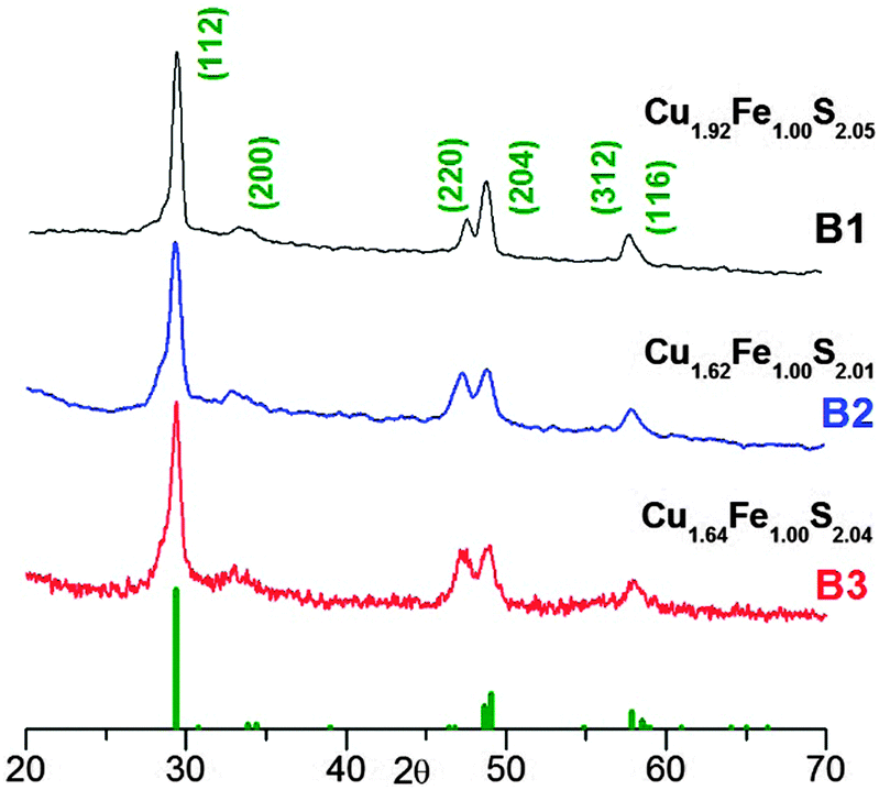Fig. 1 The X-ray diffractograms of the Cu–Fe–S nanocrystals obtained for a fixed precursor ratio (Cu : Fe : S = 1 : 1 : 2) and varying ligand (OA) to precursor ratios: OA : Cu = 3.9 (B1); OA : Cu = 2.1 (B2); OA : Cu = 1 : 1.2 (B3). The green bars indicate the diffraction pattern of chalcopyrite CuFeS₂ (JCPDS 37-0471).

B1 nanocrystals (Cu_1.92Fe_1.00S_2.01) were spherical in shape and very small (diameter of 2.9 ± 0.4 nm). B2 and B3 nanocrystals of very similar composition showed however a different morphology. The former, spherical- or cubic-type in shape were of slightly smaller size than the B1 nanocrystals (diameter of 2.7 ± 0.3 nm), the latter were much larger and tetrahedral in shape (edge size of 9.3 ± 1.7 nm) (Table 1, Fig. 2). Both shapes were isotropic yielding the aspect ratio of 1.

Fig. 2 TEM and enlarged TEM images of the Cu–Fe–S nanocrystals obtained for a fixed precursor ratio (Cu : Fe : S = 1 : 1 : 2) and varying ligand (OA) to precursor ratios: OA : Cu = 3.9 (B1); OA : Cu = 2.1 (B2); OA : Cu = 1 : 1.2 (B3).

Thus, the concentration of ligand molecules in the reaction mixture has a profound effect on the nanocrystals size. For higher concentrations, this effect was very small, below a certain OA to precursor ratio, an abrupt increase in the nanocrystals size was observed.

By varying the metal to precursor ratio in the reaction mixture, it was possible to obtain either Cu-rich or Fe-rich nanocrystals (see Fig. S1, ESI† for the corresponding Cu, Fe and S EDS spectra and Table 1 for nanocrystals compositions derived from these spectra). For the nanocrystals prepared with a Cu : Fe ratio = 4.0 : 1.0, the increase in the copper content was very pronounced (B4, composition: Cu_4.20Fe_1.00S_3.20). A weaker effect was observed for the inversed precursor ratio (Cu : Fe = 1.0 : 4.0), i.e. in the resulting nanocrystals, a smaller increase in the iron content was observed (B5, composition: Cu_1.00Fe_1.79S_2.27). This finding indicates the higher reactivity of CuCl when compared to FeCl₃ under the applied conditions of nanocrystal nucleation and growth.

Similarly as all the Cu–Fe–S nanoparticles prepared with high OA to precursor ratios, the B4 and B5 nanocrystals were spherical in shape and small (diameters of 1.5 ± 0.4 nm and 2.3 ± 0.4 nm for B4 and B5 nanocrystals, respectively), as evidenced from their TEM images presented in Fig. 3 and 4. In the same figures, their X-ray diffractograms are shown. B4 nanocrystals revealed a different crystal structure than the other four batches studied with a set of reflections at 27.0°, 28.6°, 32.8°, 34.2°, 47.1° and 55.9° corresponding to the planes indexed as (311), (222), (400), (331), (440) and (622) in the high bornite structure of Cu₅FeS₄ (JCPDS 34-0135). B5 nanocrystals, similarly as those of B1–B3 batches showed the structure of chalcopyrite (JCPDS 37-0471).

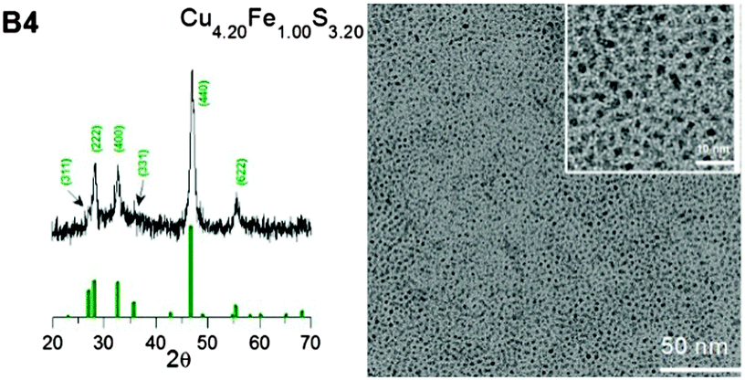Fig. 3 X-ray diffractogram (high bornite structure, JCPDS 34-0135) and TEM image (and enlarged TEM image) of the B4 nanocrystals.

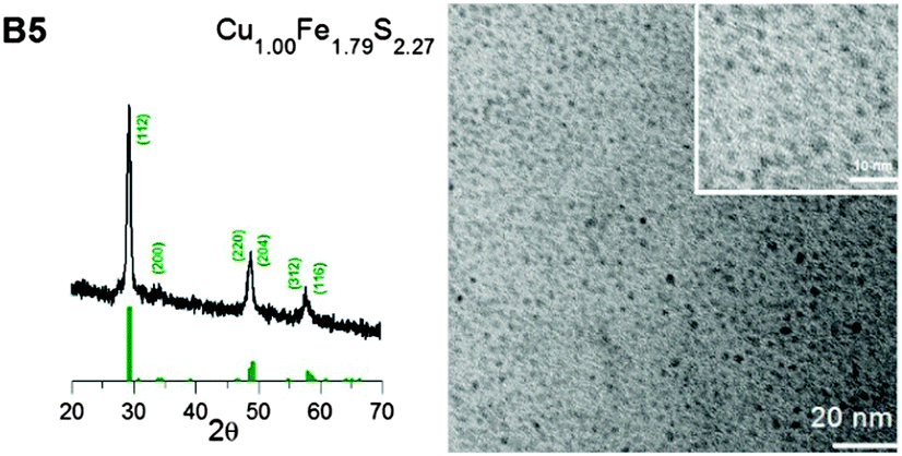Fig. 4 X-ray diffractogram (chalcopyrite structure, JCPDS 37-0471) and TEM image (and enlarged TEM image) of the B5 nanocrystals.

3.3 XPS spectroscopy

Detailed comparative studies were carried out for B2 and B3, i.e. nanocrystals showing essentially the same composition (Cu_1.62Fe_1.00S_2.01 and Cu_1.64Fe_1.00S_2.04), the same crystal structure but significantly differing in size. In Fig. 5, the high resolution Cu2p, Fe2p and S2p XPS spectra, registered for the B2 and B3 nanocrystals are compared. The high-resolution Cu2p spectra of both types of nanocrystals are similar. The doublets at ca. 932.3–932.6 eV (Cu2p_3/2) and 952.2 eV (Cu2p_1/2) can be unequivocally attributed to the presence of Cu(I).³⁰ There is no spectroscopic evidence for the presence of Cu(II), as no peak in the vicinity of 942 eV (Cu2p_3/2), characteristic of this oxidation state of copper, was detected.³¹ The high-resolution Fe2p spectra give, however, clear evidence of co-existing Fe(II) and Fe(III). This is manifested by a shift in the Fe2p doublet components to ca. 710.6–711.2 eV (Fe2p_3/2) and 723.9–724.5 eV (Fe2p_1/2) when compared to the corresponding peaks in the spectrum of bulk chalcopyrite-Cu(I)Fe(III)S₂ (708.8 (Fe2p_3/2) and 722.1 (Fe2p_1/2)).³² Note that this shift is slightly more pronounced in the case of the B3 nanocrystals.

Fig. 5 High-resolution Cu2p, Fe2p and S2p XPS spectra of B2 (blue) and B3 (red) Cu–Fe–S nanocrystals.

The S2p spectra of the B2 and B3 nanocrystals differ in a more pronounced manner. In both cases, two peaks can be distinguished at 162.2 and 168.7 eV, attributable to the sulfide form (S²⁻)³¹ and oxidized forms of sulfur (SO_x²⁻, x = 3, 4),³³ respectively. For the B2 nanocrystals, which are smaller in size than the B3 ones, the relative intensity of the peak ascribed to the oxidized forms of sulfur is higher. Partial oxidation of surfacial sulfur atoms is a common phenomenon in metals sulfide nanocrystals^33–35 and in some cases can be desirable. For example, the presence of oxidized forms of sulfur on the surface of PbS nanocrystals used for the fabrication of photodetectors resulted in an improvement in device performance.³³

As already stated, the Fe2p XPS spectra seem to indicate the co-existence of Fe(III) and Fe(II) in the B2 and B3 nanocrystals. It is tempting to verify this conclusion by ⁵⁷Fe Mössbauer spectroscopy since this is the most sensitive technique used for the detection of non-equivalent forms of iron.

3.4 Magnetic properties and Mossbauer spectroscopy

Among the different forms of Cu–Fe–S nanocrystals, one can distinguish antiferromagnetic α-CuFeS₂ (tetragonal),^36–38 ferromagnetic β-CuFeS₂ (cubic)^36,39 and non-magnetic (down to 78 K) γ-CuFeS₂ (tetragonal)³⁶ phases of chalcopyrite, ferromagnetic CuFe₂S₃ (cubanite; orthorhombic)⁴⁰ and non-magnetic cubic form of cubanite, namely, isocubanite.⁴¹ The point is how to distinguish between chalcopyrite (and its different phases) and cubanite (and its different phases). The diffraction method fails since, for instance, ferromagnetic chalcopyrite and non-magnetic isocubanite yield essentially the same set of Bragg reflections and only Mössbauer spectroscopy can help in distinguishing between these phases.^42,43 The spectra obtained for both the B2 and B3 nanoparticles are shown in Fig. 6. In both cases, even at 16 K, only a non-magnetic component in the spectrum (quadrupole doublet) can be distinguished with no evidence of the Zeeman sextet, indicating magnetic ordering. However, below 10 K, the spectra change dramatically for both sizes of nanoparticles and show a very clear Zeeman splitting.

Fig. 6 ⁵⁷Fe Mössbauer spectra of the Cu–Fe–S nanocrystals (batches B2 and B3), registered at varying temperatures (6, 10, 16 and 78 K).

At sufficiently low temperature, i.e., at 6 K, the magnetic component of the broadened lines dominates the spectra and the quadrupole doublet practically disappears. Actually, there are two possible interpretations of the observed phenomenon:

(a) B2 and B3 nanoparticles are ferromagnetic/ferrimagnetic, however, they show very strong superparamagnetism, i.e. very low blocking temperature, which is not surprising for so small nanocrystals (2.7–9.3 nm),

(b) B2 and B3 nanoparticles are antiferromagnetic showing a macroscopic quantum effect for the slowly relaxing macrospins of the magnetic sublattices.⁴⁴

Basically, both the B2 and B3 nanoparticles could be magnetic (ferro-, ferri, antiferro- or antiferri-) of very low Curie/Neel temperature and therefore known as paramagnetic (i.e., never measured below liquid nitrogen temperature). Line broadening in this case could be a result of different Fe sublattices and substituting Cu, and thus forming different chemical surroundings contributing differently to the measured Mössbauer spectra. However, the spectra shown in Fig. 6 do not show any continuous transition from the Zeeman sextet to the quadrupole doublet via decreased splitting with increasing temperature. Therefore, such interpretation does not seem to be valid. Even then it is difficult to propose a final interpretation since the spectra measured for both ferromagnetic (β-CuFeS₂) and antiferromagnetic (α-CuFeS₂) nanoparticles are expected to be qualitatively similar. Note that ferro/ferri and antiferro/antiferri states cannot be distinguished from the Mössbauer spectra even for the bulk material if the spectra are measured with no external magnetic field applied.

More precisely, in the case of ferromagnetic nanoparticles, the collapse of a low temperature well-resolved hyperfine magnetic structure in the spectrum into a quadrupole doublet should be accompanied by a line broadening at intermediate temperatures. Moreover, superparamagnetic spectra obtained at the same temperature should be strongly dependent on the size of the ferromagnetic nanoparticles. This is not the case (see Fig. 6): almost the same spectra are measured at 10 K for both the 2.7 and 9.3 nm nanoparticles. The spectral lines remain “narrow” and only the relative contribution of the well-resolved magnetic structure and the quadrupole doublet/doublets changes rapidly with increasing temperature. This may suggest the presence of antiferromagnetic α-CuFeS₂ (chalcopyrite) in these extremely small size nanocrystals, which leads to a macroscopic quantum effect. The quantum nature of the effect is concluded from the well-defined energy states (resulting from the quantum confinement phenomena for electrons in nanoparticles) of populations, which are temperature dependent.⁴⁴ In the case of ferromagnetic particles, the ground state represents a quasi-continuous spectrum independent of the anisotropy constant, whereas it is strongly anisotropy dependent in the case of the antiferromagnetic nanoparticles (small anisotropy allows the coupling between sublattice magnetizations to be strong).

Considering the antiferromagnetic state is observed only at very low temperatures, one should also remember that the Neel temperature is usually drastically suppressed with decreasing size of the antiferromagnetic particles (the finite-size effect).⁴⁵

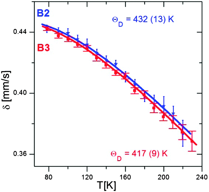
In Fig. 7, the Mössbauer spectra obtained at 78 K for B2 and B3 are compared. The doublet of the broadened spectral lines can be fitted using four components of equal contributions exhibiting slightly different splitting parameters (see Fig. 7). This type of fit helps to obtain the hyperfine parameters precisely. The measured isomer shift (δ) is the same for the nanocrystals of both batches (0.442 mm s⁻¹vs. α-Fe), whereas the quadrupole splitting (Q.S.) values slightly differ, being 0.78 mm s⁻¹ and 0.82 mm s⁻¹ for the B2 and B3 nanocrystals, respectively. This is not surprising since the δ reflects the chemical composition, which is independent of the particle diameter, whereas the Q.S. reflects symmetry of charge distribution, which could vary for the different size of nanoparticles.

Fig. 7 ⁵⁷Fe Mössbauer spectra of the Cu–Fe–S nanocrystals (batches B2 and B3), registered at 78 K.

The analysis of δ and Q.S. can be helpful in phase identification. Isomer shift values determined from the Mössbauer spectra of the B2 and B3 nanocrystals are very high for Fe(III) and very low for Fe(II),⁴¹ implying an intermediate iron oxidation state, which can be achieved though the fast electron exchange between these two form of iron.⁴⁰ Very similar Mössbauer parameters were recently reported for nanocrystals of isocubanite (known as non-magnetic but never magnetically tested at very low temperatures).⁴⁶ The chemical composition of Cu-rich B2 and B3 nanocrystals (Cu_1.62Fe_1.00S_2.01 and Cu_1.64Fe_1.00S_2.04, respectively) is however very different from that of a Fe-rich cubanite (CuFe₂S₃).

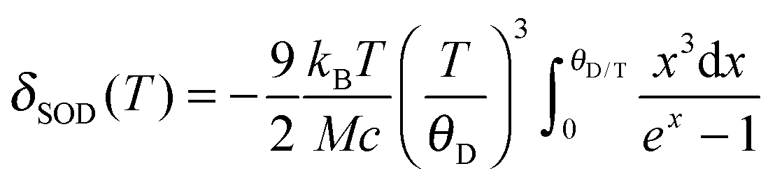
From the temperature dependence of the Mössbauer spectrum parameters, using eqn (1) and (2), it is possible to calculate the Debye temperature, θ_D, characterizing the lattice dynamics of the nanocrystalline materials studied.

δ(T) = δ₀ + δ_SOD(T) (1)

where δ(T) is the temperature dependence of the spectrum gravity center, δ₀ is the isomer shift, δ_SOD is the second order Doppler shift, M is the mass of the ⁵⁷Fe atom, c is the velocity of light and θ is the Debye temperature.

Fig. 8 shows the temperature dependence of δ, determined from the Mössbauer spectra of the B2 and B3 nanocrystals registered at different temperatures. The obtained Debye temperature values (432 K and 419 K for B2 and B3 nanocrystals, respectively) are higher by 70 to 150 K than those determined experimentally for bulk Cu–Fe–S crystals,⁴⁷ including the results obtained by Mössbauer spectroscopy.³⁸ Theoretical calculations also lead to values below 300 K.⁴⁸ Note that consistent with these findings, the value of θ obtained for the smaller B2 nanocrystals is higher than that found for the larger B3 nanocrystals. An increase in the Debye temperature with decreasing nanocrystals size was also observed for binary semiconducting CdS⁴⁹ and CdTe⁵⁰ nanocrystals. In contrast, for PbS nanocrystals, a different behavior was reported, namely, the bimodal dependence of the Debye temperature on the nanocrystals size.⁵¹ With decreasing nanocrystal size, the Debye temperature initially increased, as in the case of CdS and CdTe, but below a given “critical” size, it suddenly started to decrease.

Fig. 8 Temperature dependences of δ measured for B2 and B3 nanocrystals together with the best fit to eqn (1) and (2).

3.5 Organic ligands identification and characterization

In addition to the detailed characterization of the inorganic core, identification of the surfacial ligands is of crucial interest since their chemical nature determines the nanocrystals interactions with the environment. This is not a trivial problem since IR spectroscopy provides rather limited information in this respect, similarly as NMR spectroscopy since coordination of the ligands molecules on the nanocrystals surface leads to a significant lines broadening in the spectra.⁵²

In the identification of the initial surfacial ligands in ternary Cu–Fe–S nanocrystals, we applied the method previously elaborated in our group.²⁷ It consists of the recovery of surfacial ligands through selective dissolution of the inorganic core with HCl. Fig. 9 shows the ¹H NMR spectra of the ligands recovered from the B2 and B3 nanocrystals together with the spectra of pure 1-octadecene (ODE), oleic acid (OA) and oleylamine hydrochloride (OLA-HCl), which are added for comparative reasons. In the spectrum of the organic part of the B2 batch, a clear signal ascribed to OLA-HCl can be distinguished at 5.4 ppm and 2.9 ppm, the former originating from the vinyl protons (–CH=CH–) and latter from protons of the methylene group adjacent to the protonated amino group (–CH̲_2̲NH₃⁺). No evidence of the presence of oleic acid as a ligands can be found in the spectrum since its diagnostic signal, originating from protons of methylene group adjacent to the carboxylic one (CH̲_2̲COOH), cannot be found at 2.3 ppm. In addition, in the spectral range of 4.5–6.0 ppm, very weak signals attributed to ODE can be identified. In the spectrum of the organic part of the B3 nanocrystals, the same set of signals is present; however, the contribution of the ODE signals is more significant.

Fig. 9 ¹H NMR spectra of the organic residue recovered after the selective dissolution of the inorganic cores of the Cu–Fe–S nanocrystals (B2 and B3), 1-octadecene (ODE), oleic acid (OA) and oleylamine hydrochloride (OLA-HCl).

The IR spectra of the recovered organic shell of the synthesized nanocrystals (Fig. S3 of ESI†) are perfectly consistent with the ¹H NMR results. In addition to the bands at 2921 and 2861 cm⁻¹ attributed to the C–H stretching vibrations in the methylene groups of the aliphatic chains bands, characteristic of OLA (at 1628 cm⁻¹ and 1575 cm⁻¹) and ODE (1462 cm⁻¹, 1401 cm⁻¹ and 905 cm⁻¹) can be distinguished.

From the abovementioned results, it can be concluded that between the two components of the reaction mixture, which contain coordinating groups (OA and OLA), only OLA is bound to the nanocrystal's surface as an initial ligand. The presence of ODE requires some comments since in the elaborated preparation procedure, this chemical is not added to the reaction mixture. Therefore, it has to be formed in situ from OLA via an elimination–hydrogenation reaction occurring between OLA and the nanocrystal surface. This reaction is strongly dependent on the concentration of oleic acid (OA). In the preparation of the B3 nanocrystals, whose spectrum shows a higher amount of ODE than that of B2, a significantly smaller concentration of OA was used (see Table 1 and Table S1, ESI†).

In situ generation of ODE has already been observed in the preparation of cobalt nanocrystals involving OLA as a solvent^53,54 and in the case of the synthesis of kesterite-type Cu₂ZnSnS₄ nanoparticles.⁵⁵

The hydrodynamic diameter is another parameter characterizing nanocrystals capped with organic ligands. It describes the effective diameter of a nanocrystal, which includes the inorganic core and ligands coordinated to it. By comparison with the nanoparticle diameter determined from the TEM images, it provides information concerning the thickness of the organic shell. Moreover, its evolution in time can be considered as a test of the colloidal stability of the investigated nanocrystals. Dynamic light scattering (DLS), widely used in the studies of hydrodynamic diameters of macromolecular compounds can also be applied in the case of nanocrystals stabilized with organic ligands.^56,57 In Fig. 10 the histograms of hydrodynamic diameters determined by DLS are shown for the B2 and B3 nanocrystals dispersions in chloroform. For comparison, their average diameters obtained by statistical treatment of the TEM images are indicated. In the case of the B2 nanocrystals, the obtained DLS results are very consistent with the TEM images; their hydrodynamic diameter (6–9 nm) is more than two times larger than the average inorganic core diameter (2.7 ± 0.3 nm). This is caused by the fact that in the dispersion in chloroform, not only ligands but also some solvent molecules, penetrating the organic shell of the nanocrystals, constitute additional components in the coordination sphere. The obtained hydrodynamic diameter values of the B2 nanocrystals are also consistent with the values determined by DLS for other families of nanocrystals of comparable core and ligand size.^56,57 The colloidal solutions were stable as demonstrated by repeated DLS measurements, carried out within few days of each other, which did not show an increase in their hydrodynamic diameter.

Fig. 10 Histograms of the hydrodynamic diameters (derived from DLS studies) of the B2 and B3 nanocrystals dispersed in chloroform. The arrow parallel to the y-axis shows the average diameter of the inorganic core as determined from the TEM images.

For the B3 nanocrystals, the measured hydrodynamic diameter is unusually large, 10 to 20 nm larger than the diameter of the inorganic core. Such a big difference cannot be justified by the thickness of the organic shell, even if the penetration of the solvent to it is considered. It is therefore highly probable that in chloroform solution, the B3 nanocrystals form small agglomerates composed of a few nanoparticles.

3.6 Optical properties

The UV-vis-NIR absorption spectra of the B2 and B3 nanocrystals dispersions in chloroform are presented in Fig. 11. In the spectrum of the larger nanocrystals (9.3 ± 1.7 nm, B3 batch), a distinct peak is observed at 498 nm, which could be tentatively ascribed to the presence of surface plasmons. Such plasmonic absorptions were observed for non-stoichiometric Cu_2−xS⁵⁸ or Cu_2−xSe⁵⁹ nanocrystals, however, in the near infrared part of the spectrum. They were also reported for heterogeneous quaternary Cu–Zn–Sn–S nanocrystals,⁶⁰ where a separate Cu_2−xS phase was detected and in ternary Cu–Fe–S nanocrystals.²⁵ The position of the absorption peak in the spectrum of B3 excludes the presence of the Cu_1.98S phase, which is consistent with the X-ray diffraction data. However, it should be noted that absorption peaks in the same visible spectral range were previously reported for Cu₅FeS₄⁶¹ and alloyed quaternary Cu–Zn–Fe–S⁶² nanocrystals. The authors gave no attribution of these peaks. Our attribution of the observed absorption in the UV-vis spectrum of B3 should be treated as one of the plausible explanations only. Further investigations are needed to fully elucidate this problem. For the smaller nanocrystals (2.7 ± 0.3 nm, B2 batch), this peak is non-existent.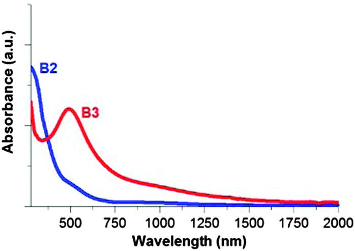

Fig. 11 NIR-vis spectra of the B2 and B3 nanocrystals dispersed in chloroform.

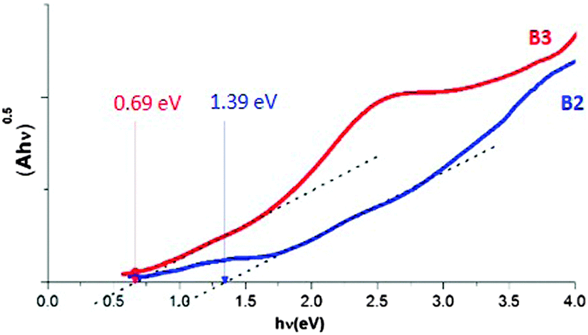
The absorption edge, as determined from the (Ahν)^0.5vs. hν dependence (see Fig. 12), yields an optical band gap of 0.69 eV for the B3 nanocrystals (9.3 ± 1.7 nm), close to the value measured for bulk CuFeS₂.³² For the smaller B2 nanocrystals (2.7 ± 0.3 nm) the optical band gap increases to 1.39 eV, indicating the quantum confinement effect.

Fig. 12 (Ahν)^0.5vs. hν relationship used for the optical band gap determination.

The band gaps, E_g, were calculated using the (Ahν)^0.5vs. hν relationship (where A = absorbance, h = Planck's constant and ν = frequency). In the majority of publications devoted to inorganic semiconductors, a direct optical band gap is estimated from the (Ahν)²vs. hν relationship. This method is less precise and ambiguous. Detailed justification for the preferable use of (Ahν)^0.5vs. hν relationship can be found in the work of Markus Meinert and Günter Reiss.⁶³

3.7 Electrochemical properties

To verify whether the quantum confinement effect is reflected in the redox properties of the prepared nanocrystals, we conducted cyclic voltammetry investigations of their colloidal dispersions in dichloromethane. Representative cyclic voltammograms of the B2 and B3 nanocrystals are shown in Fig. 13. In the case of the B2 nanocrystals, a clear oxidation peak with an irreversible nature and a very weak reduction peak at negative potentials can be distinguished (Fig. 13b). This is typical of the majority of semiconductor nanocrystals in which the oxidation processes are much more pronounced than the reduction ones.^64,65 From the potentials of the onset of oxidation and reduction peaks determined from the voltammograms of B2 and B3 (see Fig. S4 and S5, ESI†), the HOMO and LUMO energies can be determined using eqn (3) and (4).⁶⁶

E_HOMO = −(E^ox + 5.1) (eV) (3)

E_LUMO = −(E^red + 5.1) (eV) (4)

where E^ox and E^red are the potentials of the onsets of the oxidation and reduction peaks with respect to Fc/Fc⁺.

Fig. 13 (a) Cyclic voltammograms of the colloidal dispersions of the B2 (blue) and B3 (red) nanocrystals in dichloromethane, (b) the cyclic voltammogram of the colloidal dispersion of the B2 nanocrystals in dichloromethane registered in the negative potentials range. Scan rate = 50 mV s⁻¹, electrolyte 0.1 M Bu₄NBF₄ in dichloromethane, reference electrode Ag/0.1 M Ag⁺ in acetonitrile.

The electrochemical data are collected in Table 2, together with the determined HOMO and LUMO energies and the electrochemical and optical band gaps. The electrochemical band gaps (0.74 eV and 1.54 eV for B3 and B2, respectively) are slightly higher than the optical ones (0.69 eV and 1.39 eV). This is caused by the additional Coulombic repulsion energy of the exciton electron and hole, which has to be taken into account during the electrochemical measurements.⁶⁵

Table 2 The redox potentials (measured vs. the Ag/Ag⁺ electrode and Fc/Fc⁺ couple) and electrochemically determined HOMO, LUMO and E_g for B2 and B3

	E ox(onset) [V] (Ag/Ag^+)	E red(onset) [V] (Ag/Ag^+)	E ox(onset) [V] (Fc/Fc^+)	E red(onset) [V] (Fc/Fc^+)	HOMO [eV]	LUMO [eV]	E g [eV]	E g [eV]
a The electrochemical band gap. b The optical band gap.
B2	0.720	−0.817	0.570	−0.967	−5.67	−4.13	1.54	1.39
B3	0.570	−0.170	0.420	−0.320	−5.52	−4.78	0.74	0.69

---

In the case of chalcopyrite Cu–Fe–S nanocrystals, the HOMO can be considered as a combination of Cu3d–S2p, whereas the LUMO can be consider as the Fe3d–S2p orbitals.³² The electrochemical data show that the HOMO in the B2 nanocrystals is lowered by ΔE = 0.15 eV when compared to the case of the B3 nanocrystals due to the quantum confinement effect, whereas the LUMO is increased by ΔE = 0.65 eV. The more pronounced effect of quantum confinement on the LUMO energy has already been reported for chalcopyrite-type CuInS₂ nanocrystals.^67,68 This effect can be rationalized by the differences in the effective mass of electrons (m_e*) and holes (m_h*). Considering the 1S(e) (LUMO) and 1S(h) (HOMO) levels as functions of 1/m_e* and 1/m_h* (where m_e* < m_h*), the LUMO energy has to be affected in a more pronounced manner by the diminishing nanocrystal size when compared to the HOMO.

4. Conclusions

To summarize, we elaborated a new heating up method used for the preparation of ternary Cu–Fe–S nanocrystals yielding nanoparticles with different composition (from Cu-rich to Fe-rich), structure (chalcopyrite or high bornite) and size, including the smallest nanocrystals ever reported for this group (below 3 nm). For nanocrystals of the same structure and composition but differing size (2.7 nm and 9.3 nm), the quantum confinement effect was confirmed using three different techniques: UV-vis spectroscopy, cyclic voltammetry and the Mössbauer effect. NMR investigation of the organic shell revealed two coexisting ligands, namely, oleylamine (OLA) and 1-octadecene (ODE), the latter being formed in situ via an elimination–hydrogenation reaction occurring between OLA and the nanocrystal surface.

Acknowledgements

J. Ż. and M. P. are grateful to Prof. S. M. Dubiel for providing us with his spectrometer for the Mössbauer experiments at very low temperature. This research was conducted in the framework of the project entitled “New solution processable organic and hybrid (organic/inorganic) functional materials for electronics, optoelectronics and spintronics” (Contract No. TEAM/2011-8/6), which is operated within the Foundation for the Polish Science Team Programme co-financed by the EU European Regional Development Fund. One of the authors (P. B.) wants to acknowledge the partial financial support of the Warsaw University of Technology. P. Bujak and A. Pron additionally acknowledge the financial support of the National Science Centre (Poland) through the Grant No. UMO-2013/09/B/ST5/03521.

References

1. A. L. Efros, Sov. Phys. Semicond., 1982, 16, 772–775.
2. A. Henglein, Ber. Bunsenges Phys. Chem., 1982, 86, 301–305.
3. A. J. Bard, J. Phys. Chem., 1982, 86, 172–177.
4. D. V. Talapin, J.-S. Lee, M. V. Kovalenko and E. V. Shevchenko, Chem. Rev., 2010, 110, 389–458.
5. C. B. Murray, D. J. Norris and M. G. Bawendi, J. Am. Chem. Soc., 1993, 115, 8706–8715.
6. M. A. Hines and P. Guyot-Sionnest, J. Phys. Chem., 1996, 100, 468–471.
7. I. Moreels, Y. Justo, B. De Geyter, K. Haustraete, J. C. Martins and Z. Hens, ACS Nano, 2011, 5, 2004–2012.
8. X. Yang, D. Zhao, K. S. Leck, S. T. Tan, Y. X. Tang, J. Zhao, H. V. Demir and X. W. Sun, Adv. Mater., 2012, 24, 4180–4185.
9. H. Zhong, Z. Bai and B. Zou, J. Phys. Chem. Lett., 2012, 3, 3167–3175.
10. D. Aldakov, A. Lefrançois and P. Reiss, J. Mater. Chem. C, 2013, 1, 3756–3776.
11. Y. Zhao and C. Burda, Energy Environ. Sci., 2012, 5, 5564–5576.
12. T. Bell, Strategic Metal Report, Indium & the Investment Industry., 2013.
13. K. Ramasamy, M. A. Malik and P. O'Brien, Chem. Commun., 2012, 48, 5703–5714.
14. U. Ghorpade, M. Suryawanshi, S. W. Shin, K. Gurav, P. Patil, S. Pawar, C. W. Hong, J. H. Kim and S. Kolekar, Chem. Commun., 2014, 50, 11258–11273.
15. H. Yang, L. A. Jauregui, G. Zhang, Y. P. Chen and Y. Wu, Nano Lett., 2012, 12, 540–545.
16. C. L. Burdick and J. H. Ellis, J. Am. Chem. Soc., 1917, 39, 2518–2525.
17. L. Pauling and L. O. Brockway, Z. Kristallogr., 1932, 82, 188–194.
18. T. Teranishi, K. Sato and K. Kondo, J. Phys. Soc. Jpn., 1974, 36, 1618–1624.
19. C. H. L. Goodman and A. E. Pengelly, J. Electrochem. Soc., 1956, 103, 609–610.
20. D. D. Awschalom and R. K. Kawakami, Nature, 2000, 408, 923–924.
21. H. Ohno, D. Chiba, F. Matsukura, T. Omiya, E. Abe, T. Dietl, Y. Ohno and K. Ohtani, Nature, 2000, 408, 944–946.
22. D. Liang, R. Ma, S. Jiao, G. Pang and S. Feng, Nanoscale, 2012, 4, 6265–6268.
23. A. Comin and L. Mann, Chem. Soc. Rev., 2014, 43, 3957–3975.
24. Y.-H. A. Wang, N. Bao and A. Gupta, Solid State Sci., 2010, 12, 387–390.
25. P. Kumar, S. Uma and R. Nagarajan, Chem. Commun., 2013, 49, 7316–7318.
26. P. Kumar, M. Gusain, P. S. Kumar, S. Uma and R. Nagarajan, RSC Adv., 2014, 4, 52633–52636.
27. G. Gabka, P. Bujak, M. Gryszel, K. Kotwica and A. Pron, J. Phys. Chem. C, 2015, 119, 9656–9664.
28. L. Li, A. Pandey, D. J. Werder, B. P. Khanal, J. M. Pietryga and V. I. Klimov, J. Am. Chem. Soc., 2011, 133, 1176–1179.
29. B. Koo, R. N. Patel and B. A. Korgel, J. Am. Chem. Soc., 2009, 131, 3134–3135.
30. T. Kuzuya, K. Itoh, M. Ichidate, T. Wakamatsu, Y. Fukunaka and K. Sumiyama, Electrochim. Acta, 2007, 53, 213–217.
31. L. D. Partain, R. A. Schneider, L. F. Donaghey and P. S. McLeod, J. Appl. Phys., 1985, 57, 5056–5065.
32. J. A. Tossell, D. S. Urch, D. J. Vaughan and G. Wiech, J. Chem. Phys., 1982, 77, 77–82.
33. G. Konstantatos, L. Levina, A. Fischer and W. H. Sargent, Nano Lett., 2008, 8, 1446–1450.
34. N. Zhao, T. P. Osedach, L.-Y. Chang, S. M. Geyer, D. Wanger, M. T. Binda, A. C. Arango, M. G. Bawendi and V. Bulovic, ACS Nano, 2010, 4, 3743–3752.
35. G. Gabka, P. Bujak, K. Giedyk, K. Kotwica, A. Ostrowski, K. Malinowska, W. Lisowski, J. W. Sobczak and A. Pron, Phys. Chem. Chem. Phys., 2014, 16, 23082–23088.
36. I. S. Lyubutin, C.-R. Lin, S. S. Starchikov, Y.-J. Siao, M. O. Shaikh, K. O. Funtov and S.-C. Wang, Acta Mater., 2013, 61, 3956–3962.
37. G. Donnay, L. M. Corliss, J. D. H. Donnay, N. Elliott and J. M. Hastings, Phys. Rev., 1958, 12, 1917–1923.
38. H. N. Ok, K. S. Baek and E. J. Choi, Phys. Rev. B: Condens. Matter Mater. Phys., 1994, 50, 10327–10330.
39. N. A. Eissa, H. A. Sallam, M. M. El-Ockr, E. A. Mahmoud and S. A. Saleh, J. Phys., 1976, 37, C6-793–C6-796.
40. N. N. Greenwood and H. J. Whitfield, J. Chem. Soc. A, 1968, 1697–1699.
41. I. S. Lyubutin, C.-R. Lin, S. S. Starchikov, Y.-J. Siao and Y.-T. Tseng, J. Solid State Chem., 2015, 221, 184–190.
42. R. Caye, B. Cervelle, F. Cesbron, E. Oudin, P. Picot and F. Pillard, Mineral. Mag., 1988, 52, 509–514.
43. S. Pareek, A. Rais, A. Tripathi and U. Chandra, Hyperfine Interact., 2008, 186, 113–120.
44. M. A. Chuev, Hyperfine Interact., 2014, 226, 111–122.
45. X. G. Zheng, C. N. Xu, K. Nishikubo, K. Nishiyama, W. Higemoto, W. J. Moon, E. Tanaka and E. S. Otabe, Phys. Rev. B: Condens. Matter Mater. Phys., 2005, 72, 014464.
46. P. Gutlich, E. Bill and A. X. Trautwein, Mössbauer Spectroscopy and Transition Metal Chemistry, Springer-Verlag, Berlin, Heidelberg, 2011, pp. 84–85.
47. V. Kumar, A. K. Shrivastava, R. Banerji and D. Dhirhe, Solid State Commun., 2009, 149, 1008–1011.
48. J. Łażewski, H. Neumann and K. Parlinski, Phys. Rev. B: Condens. Matter Mater. Phys., 2004, 70, 195206.
49. J. Rockenberger, L. Tröger, A. Kornowski, T. Vossmeyer, A. Eychmüller, J. Feldhaus and H. Weller, J. Phys. Chem. B, 1997, 101, 2691–2701.
50. J. Rockenberger, L. Tröger, A. L. Rogach, M. Tischner, M. Grundmann, A. Eychmüller and H. Weller, J. Chem. Phys., 1998, 108, 7807–7815.
51. K. Bian, W. Bassett, Z. Wang and T. Hanrath, J. Phys. Chem. Lett., 2014, 5, 3688–3693.
52. Z. Hens and J. C. Martins, Chem. Mater., 2013, 25, 1211–1221.
53. K. M. Nam, J. H. Shim, S. Ki, S.-I. Choi, G. Lee, J. K. Jang, Y. Jo, M.-H. Jung, H. Song and J. T. Park, Angew. Chem., Int. Ed., 2008, 47, 9504–9508.
54. S. Mourdikoudis and L. M. Liz-Marzán, Chem. Mater., 2013, 25, 1465–1476.
55. G. Gabka, P. Bujak, M. Gryszel, A. Ostrowski, K. Malinowska, G. Z. Zukowska, F. Agnese, A. Pron and P. Reiss, Chem. Commun., 2015, 51, 12985–12988.
56. T. Pons, H. T. Uyeda, I. L. Medintz and H. Mattoussi, J. Phys. Chem. B, 2006, 110, 20308–20316.
57. G. Gabka, P. Bujak, K. Giedyk, A. Ostrowski, K. Malinowska, J. Herbich, B. Golec, I. Wielgus and A. Pron, Inorg. Chem., 2014, 53, 5002–5012.
58. S.-W. Hsu, K. On and A. R. Tao, J. Am. Chem. Soc., 2011, 133, 19072–19075.
59. D. Dorfs, T. Härtling, K. Miszta, N. C. Bigall, M. R. Kim, A. Genovese, A. Falqui, M. Povia and L. Manna, J. Am. Chem. Soc., 2011, 133, 11175–11180.
60. H.-C. Liao, M.-H. Jao, J.-J. Shyue, Y.-F. Chen and W.-F. Su, J. Mater. Chem. A, 2013, 1, 337–341.
61. A. M. Wiltrout, N. J. Freymeyer, T. Machani, D. P. Rossi and K. E. Plass, J. Mater. Chem., 2011, 21, 19286–19292.
62. A. Dalui, U. Thupakula, A. H. Khan, T. Ghosh, B. Satpati and S. Acharya, Small, 2015, 15, 1829–1839.
63. M. Meinert and G. Reiss, J. Phys.: Condens. Matter, 2014, 26, 115503.
64. C. Querner, P. Reiss, S. Sadki, M. Zagorska and A. Pron, Phys. Chem. Chem. Phys., 2005, 7, 3204–3209.
65. M. Amelia, C. Lincheneau, S. Silvi and A. Credi, Chem. Soc. Rev., 2012, 41, 5728–5743.
66. C. M. Cardona, W. Li, A. E. Kaifer, D. Stockdale and G. C. Bazan, Adv. Mater., 2011, 23, 2367–2371.
67. H. Nakamura, W. Kato, M. Uehara, K. Nose, T. Omata, S. Otsuka-Yao-Matsuo, M. Miyazaki and H. Maeda, Chem. Mater., 2006, 18, 3330–3335.
68. T.-L. Li and S. Teng, J. Mater. Chem., 2010, 20, 3656–3664.

---

Footnote

† Electronic supplementary information (ESI) available: Detailed information on nanocrystals preparation and characterization, EDS, XPS, IR spectra and cyclic voltammograms. See DOI: 10.1039/c6cp01887d

---