
 Open Access Article
 This Open Access Article is licensed under a Creative Commons Attribution-Non Commercial 3.0 Unported Licence
Freezing and melting line invariants of the Lennard-Jones system
Lorenzo
Costigliola
*,
Thomas B.
Schrøder
and
Jeppe C.
Dyre
“Glass and Time”, IMFUFA, Department of Sciences, Roskilde University, Postbox 260, DK-4000 Roskilde, Denmark. E-mail: lorenzo.costigliola@gmail.com
First published on 18th April 2016
Abstract
The invariance of several structural and dynamical properties of the Lennard-Jones (LJ) system along the freezing and melting lines is interpreted in terms of isomorph theory. First the freezing/melting lines of the LJ system are shown to be approximated by isomorphs. Then we show that the invariants observed along the freezing and melting isomorphs are also observed on other isomorphs in the liquid and crystalline phases. The structure is probed by the radial distribution function and the structure factor and dynamics are probed by the mean-square displacement, the intermediate scattering function, and the shear viscosity. Studying these properties with reference to isomorph theory explains why the known single-phase melting criteria hold, e.g., the Hansen–Verlet and the Lindemann criteria, and why the Andrade equation for the viscosity at freezing applies, e.g., for most liquid metals. Our conclusion is that these empirical rules and invariants can all be understood from isomorph theory and that the invariants are not peculiar to the freezing and melting lines, but hold along all isomorphs.
1 Introduction
The phase transition from liquid to crystal and vice versa is not yet completely understood.1–3 Reasons for searching for a better understanding of freezing/melting invariants are many. One is the possibility of using freezing/melting invariance to evaluate specific system properties under conditions not easily accessible by experiments. An example could be the estimation of liquid iron's viscosity under Earth-core pressure and temperature conditions, a quantity that is necessary for developing reliable geophysical models for the core.4–6In this work several freezing line and melting line invariants, both structural and dynamical, of the Lennard-Jones (LJ) system7 are derived from isomorph theory8 and validated in computer simulations. The existence of invariances along isomorphs is used to explain the Hansen–Verlet and Lindemann freezing/melting criteria as well as the Andrade equation for the freezing viscosity for the LJ system.
Many theories have been proposed to explain freezing and melting9,10 and why certain quantities are often invariant along the freezing and melting lines. Examples of such invariants are the excess entropy, the constant-volume entropy difference between liquids and solids on melting,11–13 the height of the first peak of the static structure factor on freezing (the Hansen–Verlet freezing criterion14,15), and the viscosity of liquid metals on freezing when made appropriately dimensionless.16–18 The Lindemann19,20 melting criterion states that a crystal melts when the mean vibrational displacement of atoms from their lattice position exceeds 0.1 of the mean inter-atomic distance, independent of the pressure. This is equivalent to the invariance of 〈u2〉/rm2 along the melting line,20 where 〈u2〉 is the atomic root-mean-squared vibrational amplitude and rm is the nearest neighbor distance. The most common approaches for explaining such invariants attempt to connect them to the kinetics of the freezing/melting process. For instance, going back to Born it has been suggested that a crystal becomes mechanically unstable when 〈u2〉/rm2 exceeds a certain number.9 From this perspective, it is not easy to understand why these invariants do not hold for all systems. It is also difficult to understand why related invariants hold for specific curves in the liquid state. Thus, in an extension of what happens along the melting line of, e.g., the Lennard-Jones system, the radial distribution function is invariant along the curves at which the excess entropy Sex is equal to the two-body entropy S2.21 Diffusivity is also constant, in appropriate units, along constant Sex curves,22 implying (from the Stokes–Einstein relation) an invariance of the viscosity in appropriate units along these curves. This relationship between viscosity and excess entropy was recently confirmed by high-pressure measurements.23
A possible explanation for the invariants along the freezing and melting lines, as well as along other well-defined curves in the thermodynamic phase diagram, is given by isomorph theory.8,24–26 According to it27 a large class of liquids exists for which structure and dynamics are invariant to a good approximation along the constant–excess–entropy curves. These curves are termed isomorphs, and the liquids which conform to isomorph theory are now called Roskilde-simple (R) liquids27–32 (the original name “strongly correlating” caused confusion due to the existence of strongly correlated quantum systems). Liquids belonging to this class are easily identified in computer simulations because they exhibit strong correlations between their thermal-equilibrium fluctuations of virial and potential energy in the NVT ensemble.24,33 Isomorph theory not only offers the possibility of explaining the freezing/melting invariants without reference to the actual mechanisms of the freezing/melting process itself, but by evaluating the virial potential-energy correlation coefficient also provides a way to predict whether these invariants hold for a given liquid.
The main features of isomorph theory are summarized in Section 2 where how to identify the isomorphs of the LJ system is also shown. This is followed by a short section describing technical details of the simulations performed. The isomorph equations are used in Section 4 to show that the freezing line can be approximated by an isomorph, termed the freezing isomorph, without the need for any fitting. Section 5 deals with freezing invariants, the Hansen–Verlet criterion,14,15 and Andrade's freezing viscosity equation;16–18 Section 6 focuses on melting line invariants of the FCC LJ crystal and their connection with the Lindemann criterion.19 The last section discusses the differences between isomorph theory and other approaches used to describe liquid invariances in the past years and summarizes the main results of this work.
2 Isomorphs
An R system is characterized by strong correlations between virial and potential energy equilibrium fluctuations in the NVT ensemble,24,33i.e., by a virial potential-energy equilibrium correlation coefficient R(ρ,T) greater than 0.9: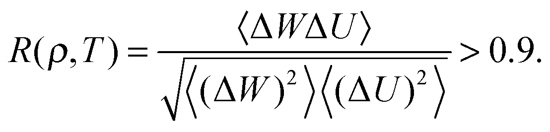 | (1) |
Reduced quantities (marked by a tilde) are defined as follows. Distances are measured in units of ρ−1/3, energies in units of kBT, and time in units of m1/2(kBT)−1/2ρ−1/3, where m is the average particle mass (for Brownian dynamics, a different time unit applies8). These reduced units should not be confused with the so-called Lennard-Jones (LJ) units. We use the latter units below for reporting quantities like temperature and density.
By definition an isomorph has the following property: for any two configurations, R1 ≡ (r(1)1,…,r(1)N) and R2 ≡ (r(2)1,…,r(2)N)
| ρ11/3R1 = ρ21/3R2 ⇒ P(R1) = P(R2) | (2) |
![[R with combining tilde]](https://www.rsc.org/images/entities/b_char_0052_0303.gif) ≡ ρ1/3R) have proportional Boltzmann factors.
≡ ρ1/3R) have proportional Boltzmann factors.
The isomorph theory is exact only for systems with an Euler-homogeneous potential energy function, for instance, inverse-power-law (IPL) pair-potential systems.24,33 However, the theory can be used as a good approximation for a wide class of systems. Examples of models that are R liquids27 in part of their thermodynamic phase diagram, in liquid and solid states,26 are the standard and generalized Lennard-Jones systems (single-component as well as multi-component),8,35,36 systems interacting via the exponential pair potential,37 and systems interacting via the Yukawa potential.28,38R systems also include some molecular systems like, e.g., the asymmetric dumbbell models,39 Lewis–Wahnström's three-site model of OTP,39 the seven-site united-atom model of toluene,24 the EMT model of liquid Cu24 and the rigid-bond Lennard-Jones chain model.40 Predictions of isomorph theory have been shown to hold for experiments on glass-forming van der Waals liquids by Gundermann et al.,41 Roed et al.,42 and Xiao et al.43 Power-law density scaling,44 which is often observed in experiments on viscous liquids, can be explained by isomorph theory.36
Isomorphic scaling, i.e., the invariance along isomorphs of many reduced quantities derived from the identical statistical weight of scaled configurations8 does not hold for all reduced quantities. For example, the reduced-unit free energy and pressure are not invariant, whereas the excess entropy, reduced structure, and reduced dynamics are all isomorph invariant.8 These invariances follow from the invariance along isomorphs of Newtonian and Brownian equations of motion in reduced units for R liquids.8
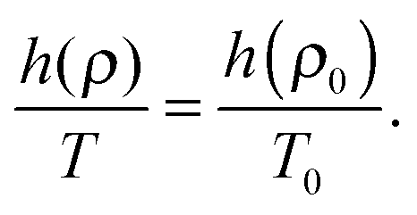
For an R system at a given reference state point (ρ0,T0), it is possible to build an isomorph starting from that point.8 For R systems, a function h(ρ) exists which relates the state point (ρ0,T0) to any other state point (ρ,T) along the same isomorph25,36 by the identity:
 | (3) |
 | (4) |
| v(r) = 4ε((r/σ)−12 − (r/σ)−6) | (5) |
 | (6) |
 | (7) |
![[thin space (1/6-em)]](https://www.rsc.org/images/entities/char_2009.gif) lnh/dlnρ25 at the reference state point to eqn (4), adopting the normalization h(ρ) = 1. The correlation coefficient R of the LJ system increases with increasing temperature and increasing density;24 this means that if the LJ system is an R liquid at the reference state point (ρ0,T0), it will be strongly correlating also at higher densities on the isomorph through (ρ0,T0).
lnh/dlnρ25 at the reference state point to eqn (4), adopting the normalization h(ρ) = 1. The correlation coefficient R of the LJ system increases with increasing temperature and increasing density;24 this means that if the LJ system is an R liquid at the reference state point (ρ0,T0), it will be strongly correlating also at higher densities on the isomorph through (ρ0,T0).
Recently isomorph theory has been reformulated starting from the assumption that for any couple of configurations of R systems, the potential energies obey the relation
| U(R1) < U(R2) ⇒ U(λR1) < U(λR2) | (8) |
3 Simulation details
This work presents the results of molecular dynamics simulations of a single-component LJ system performed using the GPU code RUMD.45 For each liquid state point an NVT simulation was used to obtain the structure and dynamics, while a SLLOD simulation46–48 was used to find the viscosity. The simulations were carried out using a shifted-potential cutoff at 2.5σ. In the simulations the LJ parameters were set to unity, i.e., σ = 1.0 and ε = 1.0. The time step was adjusted with increasing temperature along an isomorph to keep the reduced time step constant, equal to 0.001 for all simulations. For instance, the time step is 0.001 in LJ units for a simulation at ρ = 1.0 and T = 1.0. At every state point the system was simulated for 5 × 10⁸ timesteps, which takes about 20 hours (in the case of SLLOD simulations) on a modern GPU card (Nvidia GTX 780 Ti). The NVT simulations used to calculate γ and R at the starting state point for any isomorph ran for 1010 time steps in order to get good statistics for γ. In the NVT simulations of the FCC LJ crystal, the thermostat time constant was kept constant in reduced units. The value for the reduced thermostat constant is 0.4. The details of how to obtain viscosity from SLLOD simulations can be found in the Appendix. In the liquid phase and along the freezing line, 1000 LJ particles were simulated; for the FCC LJ crystal, 4000 LJ particles were simulated.4 The freezing line
As mentioned in Section 2, along an isomorph scaled configurations have the same statistical weight. This implies that the freezing and melting lines of an R liquid are isomorphs: consider a state point of the fluid state in which the disordered configurations are the most likely, and another state point in which the system is in a crystalline phase. Since in the latter case the ordered configurations are most likely, these two state points cannot be on the same isomorph. It follows that the freezing and melting lines cannot be crossed by an isomorph (in the region where the system is an R system), i.e., in both the liquid and crystalline regions isomorphs must be parallel to the freezing and melting lines, respectively. In particular, these lines are isomorphs themselves. This statement follows from assuming that the physically relevant states obey the isomorph scaling conditions.8The LJ system is an R liquid, so its freezing line is approximately an isomorph. This was first confirmed by Schrøder et al.35 using data from computer simulations by Ahmed and Sadus49 and Mastny and de Pablo,50 and subsequently by Pedersen51 with data obtained by his interface-pinning method.52 Recently, the approximate isomorph nature of the freezing line has been documented in detail by Heyes et al.53,54 The quoted papers all focus on densities fairly close to unity (in LJ units). From the fact that the freezing line is an isomorph it is possible to understand the invariance along the freezing line of several properties, as recently was shown by Heyes et al.,53 who studied the invariance of the reduced-unit radial distribution function, mean force, Einstein frequency, self-diffusion coefficient, and linear viscoelasticity of an LJ liquid along the freezing line, for densities around unity. All these quantities were found to be approximately invariant, as predicted by isomorph theory.
In this section the validity of an equation for the freezing line of the LJ system obtained from isomorph theory is checked over a considerably wider range of temperatures and densities than previously studied. In Section 5, the results of Heyes et al.53 regarding structural and dynamic invariants are extended to a wide range of densities along the freezing line.
In Fig. 1 the agreement between the freezing isomorph and the freezing line is shown to hold for the whole range of temperatures and densities studied by Agrawal and Kofke.56 The red line in Fig. 1 is the prediction from isomorph theory; this line is built by starting from the freezing point T0 = 2.0 and ρ0 = 1.063, obtained by Pedersen.51 The correlation coefficient R and the scaling parameter γ at the state point (ρ0,T0) are:
| R0 = 0.995, γ0 = 4.907. | (9) |
 | ||
| Fig. 1 Freezing line of the LJ system. In (a) the isomorph approximation to the freezing line is marked by the red line and the Khrapak and Morfill approximation55 by the black line; freezing state points obtained in the past years using various techniques are shown by symbols.49–51,56 Both approximations reproduce the data points well; the inset focuses on low densities. In (b) the relative difference between Agrawal and Kofke freezing-temperature data56 and the two approximations is shown. The isomorph approximation gives smaller deviations from the simulation data. The main advantage of approximating the freezing line by an isomorph lies, however, in the possibility of predicting the full freezing line from the knowledge of a single freezing state point. | ||
Using eqn (3) and (6) and this value for γ0, it is possible to build the freezing isomorph from
| TF(ρ) = AFρ4 − BFρ2 | (10) |
Fitting to the same simulations for the freezing line as referenced above,49,50,56 Khrapak and Morfill55 found the following values for the coefficients: A = 2.29 and B = 0.71. The line obtained inserting these values of A and B into eqn (10) is shown in Fig. 1(a) (black line). There is a significant difference in the second coefficient between the two equations. The second coefficient of Khrapak and Morfill is obtained using data for the triple point which may explain the difference; in that region isomorph theory does not provide a good approximation for the freezing line of the LJ system, as Pedersen recently showed.51 Nevertheless, the two curves are close to each other. The freezing isomorph provides a slightly better prediction of freezing temperatures at any density when compared to the Khrapak and Morfill fit (inset of Fig. 1(a) and (b)).
The main result of this section is that isomorph theory provides a technique for approximating the freezing line of an R liquid from simulations at a single state point, i.e., without any fitting, and that this approximation is valid over a wide range of densities. The relative difference between the predicted freezing temperature and the one obtained from computer simulations56 is about 6% for density change of more than a factor of 3 and temperature change of more than a factor of 100, as shown in Fig. 1. Isomorph theory allows, therefore, estimating the freezing temperatures with small relative uncertainties, and it may be useful for estimating the freezing temperatures in the high density regimes, where it is difficult to perform direct experiments for real liquids, which are R liquids in the relevant part of the phase diagram.
5 Invariants along the freezing line
In this section we discuss different invariants along the freezing isomorph as well as another isomorph “parallel” to it in the liquid state, generated from the state point (ρ,T) = (1.063,4.0). It is demonstrated that invariants originally proposed for the freezing line are also found along the liquid isomorph. Along the two isomorphs investigated, the excess pressure in reduced units is also evaluated (Fig. 2(a)). This quantity is invariant for any IPL system, but not for the LJ system. In the framework of isomorph theory, it is well understood why some quantities are invariant, e.g., the reduced viscosity, while others are not, e.g., the reduced pressure.8 This shows that the scaling properties studied in this work are not simply the consequences of an effective IPL scaling. Also note that it is necessary to go to quite high densities before γ ≈ 4, as shown in Fig. 2(b). In the same figure, the correlation coefficient R and the reduced viscosity are plotted as a function of density along the freezing isomorph. The reduced viscosity is predicted to be invariant.8 For ρ > 1.1, the reduced viscosity is invariant to a good approximation. At lower densities, the correlation coefficient R decreases and the reduced viscosity begins to vary.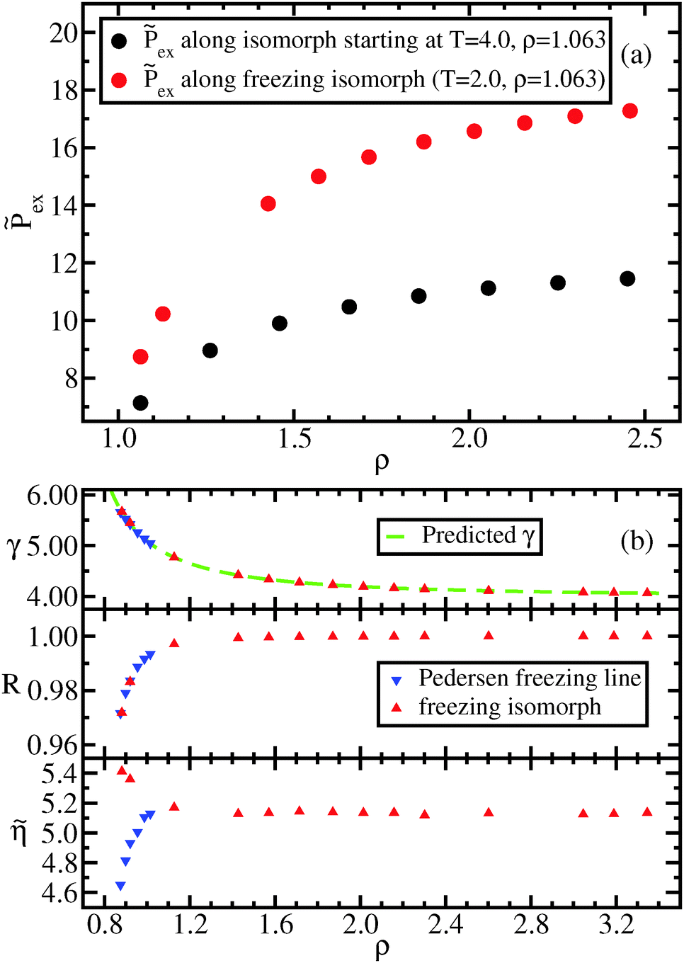 | ||
Fig. 2 (a) Excess pressure in reduced units, ![[P with combining tilde]](https://www.rsc.org/images/entities/i_char_0050_0303.gif) ex = W/(NkBT) along two different isomorphs, the freezing isomorph and a liquid isomorph. For inverse power-law pair potentials this quantity is invariant, while for the LJ system clearly it is not. This shows that isomorph scaling is not simply a trivial IPL scaling. (b) In the top panel, the scaling coefficient γ, eqn (7), is shown as a function of density along the freezing line and the freezing isomorph. The green line is the predicted value from γ = dlnh(ρ)/dlnρ.25,36 The middle and bottom panels show the virial potential-energy correlation coefficient R and the reduced viscosity ex = W/(NkBT) along two different isomorphs, the freezing isomorph and a liquid isomorph. For inverse power-law pair potentials this quantity is invariant, while for the LJ system clearly it is not. This shows that isomorph scaling is not simply a trivial IPL scaling. (b) In the top panel, the scaling coefficient γ, eqn (7), is shown as a function of density along the freezing line and the freezing isomorph. The green line is the predicted value from γ = dlnh(ρ)/dlnρ.25,36 The middle and bottom panels show the virial potential-energy correlation coefficient R and the reduced viscosity ![[small eta, Greek, tilde]](https://www.rsc.org/images/entities/i_char_e110.gif) along the freezing line and the freezing isomorph. The blue symbols mark data at freezing state points taken from Pedersen;51 the red symbols are the same quantities calculated at freezing isomorph state points. along the freezing line and the freezing isomorph. The blue symbols mark data at freezing state points taken from Pedersen;51 the red symbols are the same quantities calculated at freezing isomorph state points. | ||
5.1 Structure and the Hansen–Verlet freezing criterion
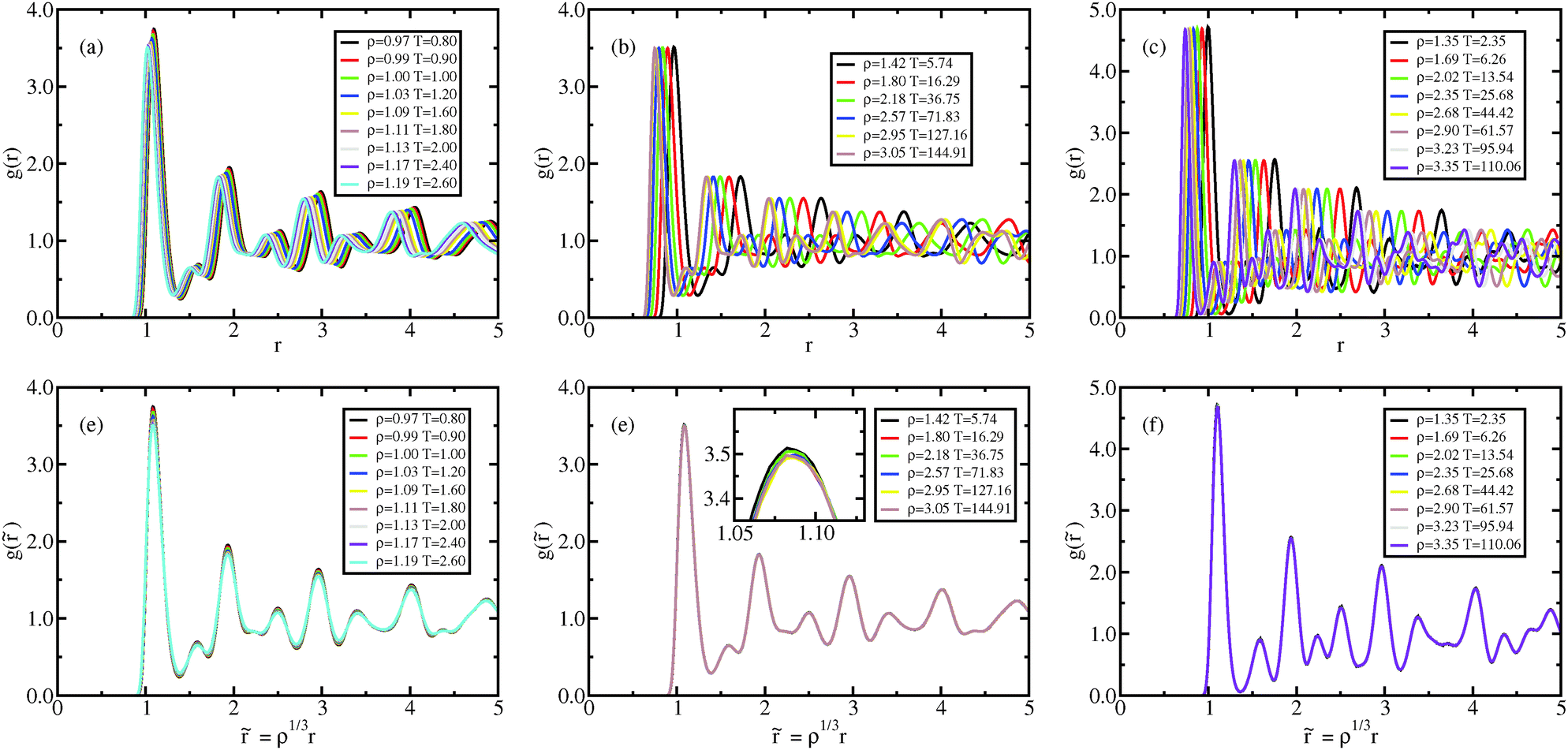
Fig. 3 shows the radial distribution functions (RDF) g(r) at different state points along the freezing line (a and d), the approximate freezing isomorph (b and e), and the liquid isomorph (c and f). In Fig. 3(a)–(c), g(r) is expressed as a function of the pair distance, while in Fig. 3(e)–(g), the g(r) is expressed as a function of the reduced distance,![[r with combining tilde]](https://www.rsc.org/images/entities/i_char_0072_0303.gif) = ρ1/3r. When the RDFs are plotted in reduced units, they collapse onto master curves, as predicted by isomorph theory. The results obtained for the freezing line confirm the recent findings of Heyes et al.,53 who showed the same collapse albeit for a smaller density range.
= ρ1/3r. When the RDFs are plotted in reduced units, they collapse onto master curves, as predicted by isomorph theory. The results obtained for the freezing line confirm the recent findings of Heyes et al.,53 who showed the same collapse albeit for a smaller density range.
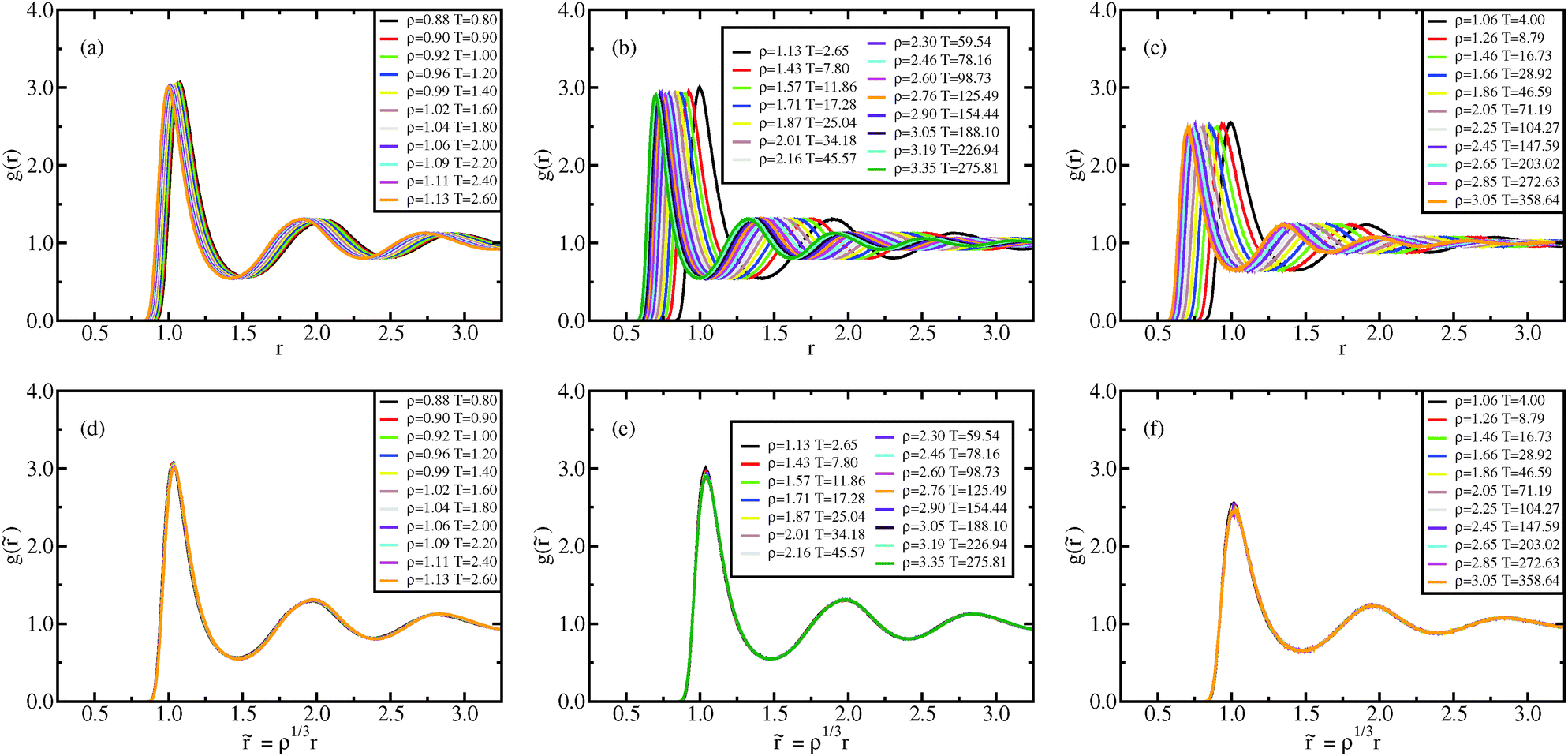 | ||
| Fig. 3 Liquid results. Radial distribution function along the Pedersen freezing line (a and d),51 along the approximating freezing isomorph (b and e) and along an isomorph well within the liquid state (c and f); in (a–c), the RDFs are plotted as a function of distance in Lennard-Jones units, in (d–f), the RDFs are plotted as a function of the reduced distance. It is worth noting that while in (a) and (d) the density change is only a few percent, in the other figures density changed by about a factor of 3. The same holds for Fig. 4–6. | ||
Starting from the invariance of g(r) it is easy to show that the structure factor S(q) is invariant when considered as a function of the reduced wave vector,
 | (11) |
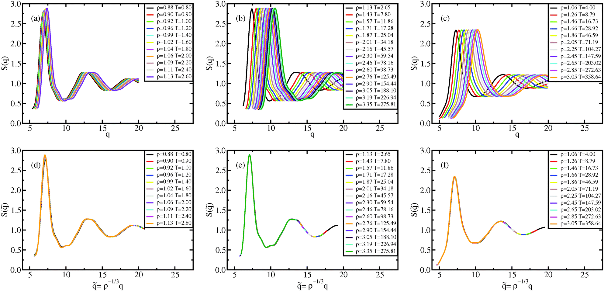 | ||
| Fig. 4 Liquid results. Structure factor along the Pedersen freezing line (a and d),51 along the approximate freezing isomorph (b and e), and along an isomorph well within the liquid state (c and f); in (a–c), S(q) is plotted as a function of wave vector in Lennard-Jones units, in (d–f), S(q) is plotted as a function of reduced wave vector. | ||
5.2 Dynamic invariants: mean-squared displacement and intermediate scattering function
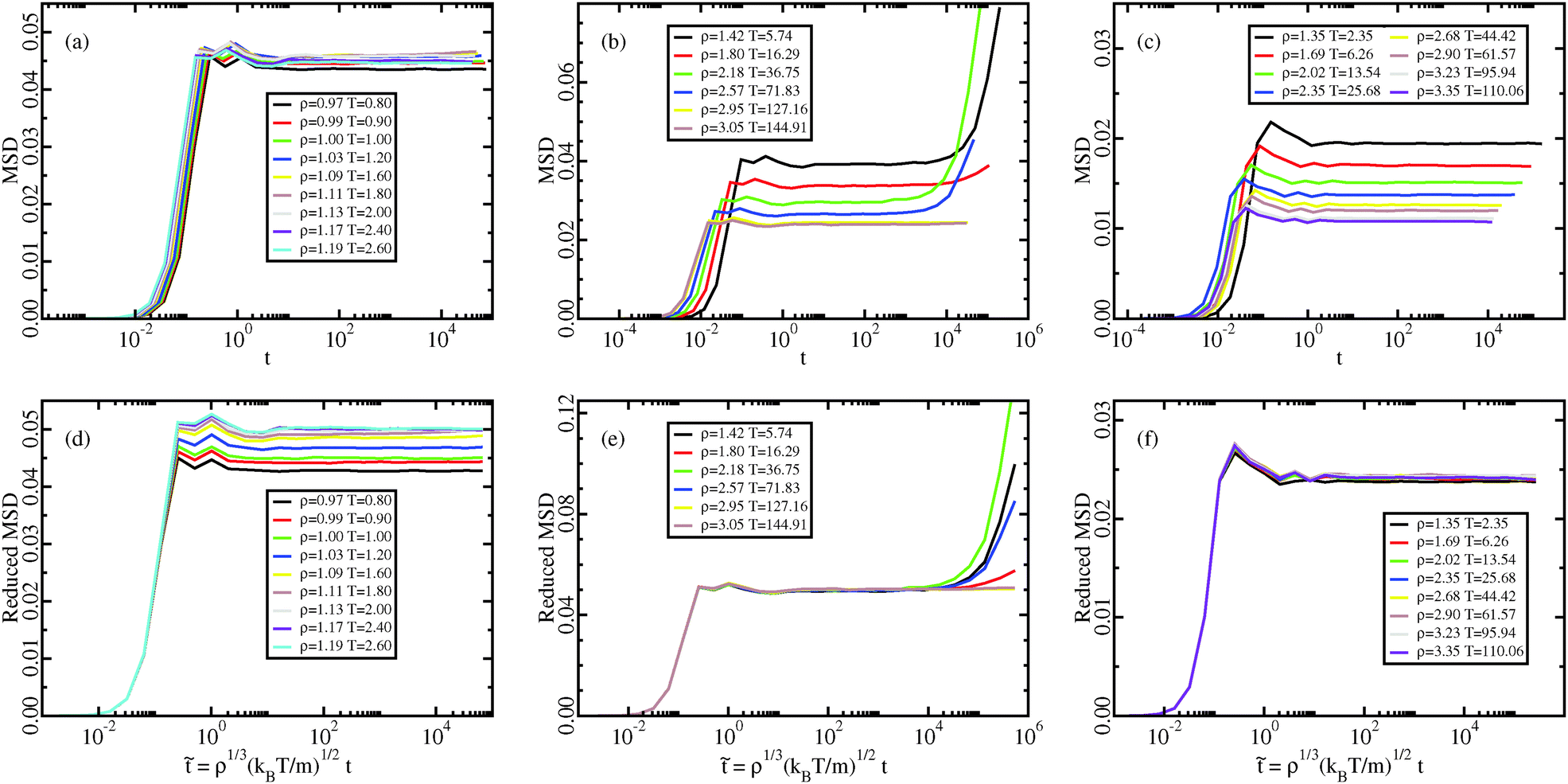
The dynamical behavior of the system is described by the mean-squared displacement (MSD) and the self-intermediate scattering function (ISF). In Fig. 5 and 6, the MSDs and ISFs are shown, respectively, as functions of non-reduced and reduced quantities. As for the structure, the curves collapse onto master curves. | ||
| Fig. 5 Liquid results. Mean-squared displacement along the Pedersen freezing line (a and d),51 along the approximating freezing isomorph (b and e) and along another isomorph in the liquid state (c and f); in (a–c), the MSDs are plotted as a function of time in LJ units, in (d–f), the reduced MSDs are plotted as a function of reduced time. | ||
 | ||
Fig. 6 Liquid results. Self-intermediate scattering function along the Pedersen freezing line (a and d),51 along the approximating freezing isomorph (b and e), and along another isomorph in the liquid state (c and f); in (a–c), the ISFs are plotted as a function of time in Lennard-Jones units, in (d–f), the ISFs are plotted as a function of reduced time. All the ISFs correspond to the q value of the first peak of S(q), qmax. The quantity ![[q with combining tilde]](https://www.rsc.org/images/entities/i_char_0071_0303.gif) max is invariant along an isomorph due to the invariance of max is invariant along an isomorph due to the invariance of ![[S with combining tilde]](https://www.rsc.org/images/entities/i_char_0053_0303.gif) (), eqn (11). (), eqn (11). | ||
5.3 Viscosity along the freezing line and the Andrade equation
In order to evaluate the viscosity the system was simulated using the SLLOD algorithm48 (details are given in the Appendix). Studies of the viscosity of the LJ system were done in the past, e.g., by Ashurst and Hoover,59 and more recently by Galliero et al.60 and Delage-Santacreu et al.,61 in all cases for densities fairly close to unity.Isomorph theory predicts the reduced viscosity to be constant to a good approximation along an isomorph (and therefore along the freezing line),
 | (12) |
 | (13) |
0 = 5.2 is the reduced value of η at the reference state point (ρ0,T0) = (1.063,2.0). Eqn (13) is identical to the Andrade equation for the freezing viscosity17,18 from 1934: | (14) |
0 in eqn (13) depends on the chosen potential.
In Fig. 7 viscosity results are compared to the values of the viscosity predicted from isomorph theory using eqn (13).
 | ||
| Fig. 7 Viscosity along the approximate freezing isomorph, eqn (10), as a function of density (a) and temperature (b). The black dots represent results for the viscosity obtained from our SLLOD simulations (Appendix). The green line is the predicted viscosity assuming the invariance of reduced viscosity along an isomorph (eqn (13)). The red dot is the viscosity of the state point from which the freezing isomorph is built and the constant of eqn (13) determined, (ρ,T) = (1.063,2.0). The reduced viscosity at this state point is 0 = 5.2. | ||
The green line in Fig. 7(b) is obtained by solving eqn (10) with respect to ρ2 and using the solution to remove the ρ dependence from eqn (13). This results in
 | (15) |
In Fig. 8 we show the reduced viscosity along the freezing isomorph as well as along the liquid isomorph with reference state point (ρ0,T0) = (1.063,4.0). The figure demonstrates that invariance of the reduced viscosity along the freezing line is not a specific property of the freezing line, but a consequence of the more general isomorph invariance.
 | ||
| Fig. 8 Reduced viscosity along the freezing isomorph and along an isomorph well within the liquid state. | ||
Andrade's equation for the freezing viscosity, which is explained by isomorph theory, was also discussed recently by Fragiadakis and Roland.63 It is interesting to compare the temperature range accessible to experiments with that of the present work. Fragiadakis and Roland63 reported data on liquid argon in a range of temperatures corresponding to [0.75,4.17] in LJ units. This is impressive, but simulations allow one to cover an even wider range of freezing temperatures.
6 Invariants along the melting line
Following the same argument as for the freezing line (Section 4), the melting line is also an approximate isomorph. A study similar to that of Section 5 was performed, evaluating the structure and MSD, for an FCC LJ crystal along the melting line as well as another isomorph in the crystalline phase. The starting point for the melting isomorph is taken from Pedersen;51 this is the state point (ρ,T) = (1.132,2.0). The starting point for the crystal isomorph is (ρ,T) = (1.132,1.0), which is well within the crystalline phase. The melting isomorph equation for the LJ system is| TM(ρ) = AMρ4 − BMρ2 | (16) |
| ρ M | T M | T pinning | ΔT/TM |
|---|---|---|---|
| 0.973 | 0.800 | 0.921 | −0.132 |
| 0.989 | 0.900 | 1.006 | −0.106 |
| 1.005 | 1.000 | 1.095 | −0.086 |
| 1.034 | 1.200 | 1.270 | −0.055 |
| 1.061 | 1.400 | 1.453 | −0.036 |
| 1.087 | 1.600 | 1.636 | −0.022 |
| 1.109 | 1.800 | 1.812 | −0.007 |
| 1.132 | 2.000 | 2.000 | +0.000 |
| 1.153 | 2.200 | 2.191 | +0.004 |
| 1.172 | 2.400 | 2.371 | +0.012 |
| 1.191 | 2.600 | 2.561 | +0.015 |
| 3.509 | 258.44 | 275.81 | +0.067 |
 | ||
| Fig. 9 Crystal results. Radial distribution function along the Pedersen melting line (a and d),51 along the approximating melting isomorph (b and e), and along an isomorph well within the crystalline state (c and f); in (a–c), the RDFs are plotted as a function of distance in Lennard-Jones units, in (d–f), the RDFs are plotted as a function of reduced distance. It is worth noting that while in (a) and (d) the density change is only a few percent, in the other figures density changed by about a factor of 3. The same holds for Fig. 10. | ||
 | ||
| Fig. 10 Crystal results. Mean-squared displacement along the Pedersen melting line (a and d),51 along the approximate melting isomorph (b and e), and along an isomorph well within the crystalline state (c and f); in (a–c), the MSDs are plotted as a function of time in LJ units, in (d–f), the reduced MSDs are plotted as a function of reduced time. The invariance of the plateau of MSD along the melting line implies the Lindemann melting criterion for R liquids because the invariance of the reduced-unit vibrational mean-square displacement in equivalent to the invariance of the Lindemann constant (Section 6). Along the melting isomorph diffusion of defects is observed. Defect formation is a stochastic phenomenon, as shown by the non-monotonicity of its appearance with respect to T or ρ. In order to study the isomorphic invariance of defect formation, it is necessary to average over many simulations at every state point and it could be the object of future studies. The diffusion of defects in crystal, when appropriately averaged, has been shown to be an isomorphic invariant by Albrechtsen et al.26 | ||
7 Discussion
We have studied several properties of the LJ model along its freezing and melting lines, as well as along isomorphs well within the liquid and crystalline phases. In Table 2 the coefficients describing the four isomorphs studied in this work are given together with the relative reference state points. The primary aim was not to report that these invariances hold, which is already well known9,14,16,66,67 albeit over smaller melting temperature/density ranges than studied here, but to relate these invariances to isomorph theory. With this goal in mind we investigated whether the invariants, thought to be peculiar to the freezing/melting process, also hold along other isomorphs in the liquid and crystalline phases. The results show that this is indeed the case. This means that these invariants are consequences of the LJ system being an R liquid in the relevant part of its phase diagram, not a specific property of freezing or melting. Nevertheless it should be stressed that invariances of reduced unit quantities, which would be exact if the freezing/melting lines were perfect isomorphs, are violated somewhat close to the triple point.| A | B | T | ρ | γ | R | |
|---|---|---|---|---|---|---|
| Liquid isomorph | 4.32 | 1.34 | 4.0 | 1.063 | 4.7589 | 0.9966 |
| Freezing isomorph | 2.27 | 0.80 | 2.0 | 1.063 | 4.9079 | 0.9955 |
| Melting isomorph | 1.76 | 0.69 | 2.0 | 1.132 | 4.8877 | 0.9985 |
| Crystal isomorph | 0.91 | 0.39 | 1.0 | 1.132 | 4.9979 | 0.9986 |
Before discussing our results in detail, we would like to point out the differences between isomorph theory and other approaches often used to describe the LJ system invariances. These other attempts to describe LJ invariances are the well-known hard sphere (HS) paradigm and the WCA (Weeks, Chandler, Andersen) approximation. The HS paradigm and isomorph theory are able to describe the nature of the same invariances, but with some important differences. A first difference is in the possibility of determining when the theory is expected to work and when it is not. In the case of isomorph theory there is a simple prescription: if the system is strongly correlating then it is possible to build isomorphs along which many reduced quantities are invariant. In the framework of hard spheres it is not possible to proceed in this way. It is not even possible to know from one single state point if some invariances will hold in the region around that state point because there is no equivalent of the correlation coefficient R defined in eqn (1). Another fundamental difference between the two approaches is the presence of an ad hoc-defined hard sphere radius that is in general state-point dependent. Isomorph theory works without the need of introducing any ad hoc parameters. A last difference, which is perhaps the most important, lies in the possibility of predicting which invariances the system will have. According to the HS paradigm, once the mapping from the studied system to the HS system is done using the ad hoc defined HS radius, the invariances of the HS system are inherited from the studied system. This means that the structure, dynamics and thermodynamic quantities should be invariant along constant-packing-fraction curves. In Fig. 2 we showed that the reduced pressure of the LJ system is not invariant along an isomorph (a) while the reduced viscosity is (b), as predicted from isomorph theory. Another possible comparison is between isomorph theory and the WCA approximation for the LJ system. While in isomorph theory there is no reference system, the WCA approximation is based on the idea that only the repulsive part of the LJ potential is relevant to the description of the system, providing a convenient reference system, and that LJ invariances can be derived from HS invariances.68
In Fig. 11(a) the viscosity is shown along the freezing line data from Agrawal and Kofke56 for the LJ system and for the IPL potential:
| νIPL(r) = 4r−12 | (17) |
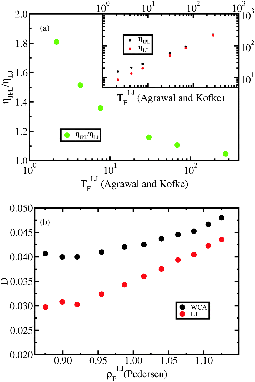 | ||
| Fig. 11 (a) Viscosities (inset) of the IPL12 system and the LJ system along the freezing line (data from Agrawal and Kofke56) and their ratio (main figure). The viscosities are calculated using the SLLOD algorithm.46–48 The viscosity of the IPL12 system is substantially different from that of the LJ system for temperatures lower than T = 68.5 in LJ units. (b) Diffusion constant for the LJ system and the WCA system along the Pedersen freezing line. It is well known that the WCA potential reproduces with good accuracy the structure of the LJ system while this is not the case for dynamics, as the figure shows. | ||
In Fig. 11(b) the diffusion constant D for the LJ system with the WCA approximation and with the 2.5σ cutoff are shown. The WCA approximation is well known to reproduce with good accuracy the structure of the LJ system, but it fails in reproducing the dynamics. Berthier and Tarjus69 already underlined that this was the case for the Kob–Andersen binary LJ system, and Pedersen et al.70 showed how isomorph theory provides a better description of the LJ system dynamics while preserving the good description of the structure.
In Sections 5 and 6 we discussed the relationship between isomorph theory and freezing/melting criteria. It was shown that the invariance along the freezing line of the maximum of the static structure factor S(q) (the Hansen–Verlet criterion) results from a general invariance along isomorphs of the entire S(q) function. The first peak of the structure factor along an isotherm decreases gradually with decreasing density. This means that there will be a specific value which corresponds to the freezing phase transition. The evidence that the value of this height is constant along the freezing line is not a peculiarity of the freezing process itself, but a consequence of isomorph scaling. The reason why the maximum height of S(q) is 2.8514,15 cannot be explained within isomorph theory, but is a feature of the freezing process. In order to explain the universality of the number 2.85, as well as the universality of the Lindemann melting criterion number, one must refer to quasiuniversality, a further consequence of the isomorph theory detailed, e.g., by Bacher et al.71 Note the compatibility of the general isomorph theory with the results of Saija et al.72 on the pair-potential dependence of the maximum height of S(q) at freezing.
The study of the LJ structure factor along the freezing line also allows explaining some properties of structure factors for liquid metals observed in X-ray experiments. As shown by Waseda and Sukuri in 1972,73 for some liquid metals the ratio of the position of the first and second peaks in the structure factor is the same while there are others for which this does not hold, for example, Ga, Sn, and Bi. The first set of metallic liquids are the ones which are R liquids (i.e., exhibit strong virial potential-energy correlations) and therefore are similar to the LJ system studied in this work, while those in the second do not, as shown very recently by Hummel et al.74 from ab initio density functional theory calculations.
Along the melting line we studied the Lindemann criterion, which has been widely discussed65,66,72,75 and also experimentally tested,76 and the same conclusion holds as for the Hansen–Verlet criterion. Isomorphs' existence implies that an R liquid's thermodynamic phase diagram becomes effectively one-dimensional with respect to the isomorph-invariant quantities. The reduction of the 2d phase diagram to an effectively 1d phase diagram is crucial for understanding the connection between isomorph theory and the Lindemann criterion, because it removes one of the main criticisms against this criterion, i.e., its being a single-phase criterion.9 If the phase diagram is effectively one-dimensional, there is a unique melting process and the Lindemann constant is the value associated with this phase transition; the invariance of the Lindemann constant along the melting line is, in this view, a consequence of isomorph invariance. This argument also explains why one can use a single-phase criterion to predict where the melting process takes place for R liquids. According to the Lindemann criterion, the crystal melts when the vibrational MSD exceeds a threshold value, which in reduced units is constant along the melting line. This condition is equivalent to the invariance of the MSD along the melting line, an isomorph prediction. Note that isomorph theory can be used to predict for which systems the Lindemann criterion (at least) must hold, namely all R liquids. Recent comprehensive density-functional theory (DFT) simulation data from Hummel et al.74 show that most metals are R liquids and therefore the Lindemann criterion must apply for them in the sense that the reduced-unit MSD is approximately invariant along the melting line. On the other hand, systems that do not exhibit strong correlations between virial and potential-energy do not necessarily obey the Lindemann criterion. Thus as discussed by Stacey and Irvine already in 1977,67 the Lindemann criterion applies for systems which “undergo no dramatic changes in coordination on melting”. This is not the case for hydrogen-bonding systems, which are not R liquids.24,27 The non-universal validity of the Lindemann criterion is also supported by Lawson66 and by Fragiadakis and Roland.63 Another interesting point is the connection between the Lindemann and Born criteria, relating melting to the vanishing of the shear modulus in the crystal. Jin et al.77 showed that for a LJ system when the Lindemann criterion is satisfied, the Born criterion78 too holds to a good approximation. In view of isomorph theory this is not surprising, because the reduced shear modulus is invariant along an isomorph and therefore constant on melting.
In Section 5 we discussed the relation between isomorph theory and Andrade's viscosity equation from 1934 for the viscosity of liquid metals at freezing. This equation is equivalent to stating invariance of the reduced viscosity along an isomorph, eqn (13) and (14). As for the Lindemann criterion, isomorph theory provides the possibility to predict whether a liquid will obey the Andrade equation. The DFT simulation data from Hummel et al.74 explain why this equation holds for liquid alkali metals (as well as other invariances79); likewise one also expects this equation to hold for many other metals, for example, iron. The last point is of significant interest because the estimation of viscosity of liquid iron close to the freezing line in the Earth core is of crucial relevance for the development of Earth-core models,4–6 but is still widely debated.80–82 Isomorph scaling predicts an increase of the real (non-reduced) viscosity along the freezing line consistent with the results of Fomin et al.81
8 Conclusions
We have shown that the freezing and melting lines are approximately isomorphs and how the isomorph theory can be used to explain why some liquids have simple behavior at freezing and melting, i.e., have several structural and dynamical approximate invariants along the freezing and melting lines. Thus this theory can be used for R liquids to determine the melting and freezing physical quantities not easily accessible by experiments, ranging from noble gases like argon to liquid metals to certain molecular liquids.A Determining the zero-strain rate viscosity from SLLOD simulations
An SLLOD simulation46–48 is a molecular dynamic simulation performed by shearing the simulation box with constant speed. Between the bottom part of the box and the top part there is a relative shearing motion with a strain rate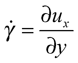 , where ux is the streaming velocity at ordinate y when the box is sheared in the x direction. Under low strain-rate conditions, this kind of simulation reproduces an ordinary, linear Coulette flow and the linear, shear-rate-independent, viscosity can be calculated from the stress tensor σij through the equation
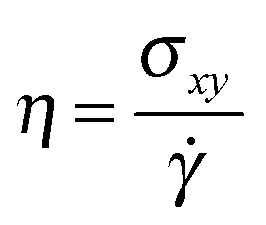 | (18) |
![[small gamma, Greek, dot above]](https://www.rsc.org/images/entities/i_char_e0a2.gif) for which the measured viscosity starts to be strain-rate dependent is isomorph invariant when given in reduced units.
for which the measured viscosity starts to be strain-rate dependent is isomorph invariant when given in reduced units.
The behavior of the reduced viscosity as a function of the reduced strain rate  is shown in Fig. 12. When the two considered state points are on the same isomorph, they exhibit the same shear-thinning behavior in reduced units; this is not true if we move along an isochore or along an isotherm. The dotted green line in Fig. 12 marks the reduced strain rate used for the simulations along the freezing line reported in the paper.
 | ||
| Fig. 12 Measured reduced viscosity from eqn (18) at different reduced strain rates. Two of the five state points (green and red dots) are on the same isomorph (the freezing isomorph of Section 4) and their behavior in reduced units is the same. As a consequence, the reduced strain rate at which reduced viscosity starts to be strain rate dependent is an isomorphic invariant, consistently with results from Separdaret al.83 The blue and violet dots are results of simulations at state points isochoric or isothermic to the (ρ,T) = (1.125,2.6). The behavior of reduced viscosity as a function of the strain rate is strongly modified changing density or temperature if the chosen state points are not isomorphic. | ||
Acknowledgements
The authors are grateful to Ulf R. Pedersen and Nicholas P. Bailey for many useful discussions. The center for viscous liquid dynamics Glass and Time is sponsored by the Danish National Research Foundation via Grant No. DNRF61.References
- R. W. Cahn, Nature, 1986, 323, 668–669 CrossRef.
- D. W. Oxtoby, Nature, 1990, 347, 725–730 CrossRef CAS.
- R. W. Cahn, Nature, 2001, 413, 582–583 CrossRef CAS PubMed.
- J.-P. Poirier, Geophys. J., 1988, 92, 99–105 CrossRef.
- J.-P. Poirier, Introduction to the Physics of the Earth's Interior, Academic, 2nd edn, 2000 Search PubMed.
- F. D. Stacey, Rep. Prog. Phys., 2010, 73, 046801 CrossRef.
- J. E. Lennard Jones, Proc. R. Soc. London, Ser. A, 1924, 106, 441–462 CrossRef.
- N. Gnan, T. B. Schrøder, U. R. Pedersen, N. P. Bailey and J. C. Dyre, J. Chem. Phys., 2009, 131, 234504 CrossRef PubMed.
- A. R. Ubbelohde, Melting and Crystal Structure, Clarendon, London, 1965 Search PubMed.
- D. C. Wallace, Statistical Physics of Crystals and Liquids, World Scientific, Singapore, 2002 Search PubMed.
- J. L. Tallon, Nature, 1989, 342, 658–660 CrossRef CAS.
- J. L. Tallon, Phys. Lett. A, 1980, 76, 139–142 CrossRef.
- S. M. Stishov, Phys.-Usp., 1975, 17, 625 CrossRef.
- J.-P. Hansen and L. Verlet, Phys. Rev., 1969, 184, 151–161 CrossRef CAS.
- J.-P. Hansen, Phys. Rev. A: At., Mol., Opt. Phys., 1970, 2, 221–230 CrossRef.
- E. d. C. Andrade, Nature, 1931, 128, 835 CrossRef.
- E. d. C. Andrade, London, Edinburgh Dublin Philos. Mag. J. Sci., 1934, 17, 497–511 CrossRef CAS.
- E. d. C. Andrade, London, Edinburgh Dublin Philos. Mag. J. Sci., 1934, 17, 698–732 CrossRef.
- F. A. Lindemann, Phys. Z., 1910, 11, 609 CAS.
- J. J. Gilvarry, Phys. Rev., 1956, 102, 308–316 CrossRef CAS.
- F. Saija, S. Prestipino and P. V. Giaquinta, J. Chem. Phys., 2001, 115, 7586–7591 CrossRef CAS.
- M. Dzugutov, Nature, 1996, 381, 137–139 CrossRef CAS.
- E. H. Abramson, J. Phys. Chem. B, 2014, 118, 11792–11796 CrossRef CAS PubMed.
- N. P. Bailey, U. R. Pedersen, N. Gnan, T. B. Schrøder and J. C. Dyre, J. Chem. Phys., 2008, 129, 184507 CrossRef PubMed.
- T. S. Ingebrigtsen, L. Bøhling, T. B. Schrøder and J. C. Dyre, J. Chem. Phys., 2012, 136, 061102 CrossRef PubMed.
- D. E. Albrechtsen, A. E. Olsen, U. R. Pedersen, T. B. Schrøder and J. C. Dyre, Phys. Rev. B: Condens. Matter Mater. Phys., 2014, 90, 094106 CrossRef.
- T. S. Ingebrigtsen, T. B. Schrøder and J. C. Dyre, Phys. Rev. X, 2012, 2, 011011 Search PubMed.
- A. A. Veldhorst, T. B. Schrøder and J. C. Dyre, Phys. Plasmas, 2015, 22, 073705 CrossRef.
- T. B. Schrøder and J. C. Dyre, J. Chem. Phys., 2014, 141, 204502 CrossRef PubMed.
- N. P. Bailey, T. B. Schrøder and J. C. Dyre, Phys. Rev. E: Stat., Nonlinear, Soft Matter Phys., 2014, 90, 042310 CrossRef PubMed.
- J. C. Dyre, Phys. Rev. E: Stat., Nonlinear, Soft Matter Phys., 2013, 87, 022106 CrossRef PubMed.
- J. C. Dyre, Phys. Rev. E: Stat., Nonlinear, Soft Matter Phys., 2013, 88, 042139 CrossRef PubMed.
- N. P. Bailey, U. R. Pedersen, N. Gnan, T. B. Schrøder and J. C. Dyre, J. Chem. Phys., 2008, 129, 184508 CrossRef PubMed.
- T. B. Schrøder, N. P. Bailey, U. R. Pedersen, N. Gnan and J. C. Dyre, J. Chem. Phys., 2009, 131, 234503 CrossRef PubMed.
- T. B. Schrøder, N. Gnan, U. R. Pedersen, N. Bailey and J. C. Dyre, J. Chem. Phys., 2011, 134, 164505 CrossRef PubMed.
- L. Bøhling, T. S. Ingebrigtsen, A. Grzybowski, M. Paluch, J. C. Dyre and T. B. Schrøder, New J. Phys., 2012, 14, 113035 CrossRef.
- A. Bacher and J. Dyre, Colloid Polym. Sci., 2014, 292, 1971–1975 CAS.
- A. A. Veldhorst, PhD thesis, Roskilde Universitet, 2014.
- T. S. Ingebrigtsen, T. B. Schrøder and J. C. Dyre, J. Phys. Chem. B, 2012, 116, 1018–1034 CrossRef CAS PubMed.
- A. A. Veldhorst, J. C. Dyre and T. B. Schrøder, J. Chem. Phys., 2014, 141, 054904 CrossRef PubMed.
- D. Gundermann, U. R. Pedersen, T. Hecksher, N. P. Bailey, B. Jakobsen, T. Christensen, N. B. Olsen, T. B. Schroder, D. Fragiadakis, R. Casalini, C. M. Roland, J. C. Dyre and K. Niss, Nat. Phys., 2011, 7, 816–821 CrossRef.
- L. A. Roed, D. Gundermann, J. C. Dyre and K. Niss, J. Chem. Phys., 2013, 139, 101101 CrossRef PubMed.
- W. Xiao, J. Tofteskov, T. V. Christensen, J. C. Dyre and K. Niss, J. Non-Cryst. Solids, 2015, 407, 190–195 CrossRef CAS.
- C. M. Roland, S. Hensel-Bielowka, M. Paluch and R. Casalini, Rep. Prog. Phys., 2005, 68, 1405 CrossRef CAS.
- N. P. Bailey, T. S. Ingebrigtsen, J. S. Hansen, A. A. Veldhorst, L. Bøhling, C. A. Lemarchand, A. E. Olsen, A. K. Bacher, H. Larsen, J. C. Dyre and T. B. Schrøder, 2015, arXiv:1506.05094.
- D. J. Evans and G. Morriss, Statistical mechanics of nonequilibrium liquids, Cambridge University Press, 2008 Search PubMed.
- P. J. Daivis and B. D. Todd, J. Chem. Phys., 2006, 124, 194103 CrossRef PubMed.
- M. Evans and D. Heyes, Mol. Phys., 1990, 69, 241–263 CrossRef.
- A. Ahmed and R. J. Sadus, J. Chem. Phys., 2009, 131, 174504 CrossRef PubMed.
- E. A. Mastny and J. J. de Pablo, J. Chem. Phys., 2007, 127, 104504 CrossRef PubMed.
- U. R. Pedersen, J. Chem. Phys., 2013, 139, 104102 CrossRef PubMed.
- U. R. Pedersen, F. Hummel, G. Kresse, G. Kahl and C. Dellago, Phys. Rev. B: Condens. Matter Mater. Phys., 2013, 88, 094101 CrossRef.
- D. M. Heyes, D. Dini and A. C. Brańka, Phys. Status Solidi B, 2015, 1–12 Search PubMed.
- D. M. Heyes and A. C. Brańka, J. Chem. Phys., 2015, 143, year CrossRef PubMed.
- S. A. Khrapak and G. E. Morfill, J. Chem. Phys., 2011, 134, 094108 CrossRef PubMed.
- R. Agrawal and D. A. Kofke, Mol. Phys., 1995, 85, 43–59 CrossRef CAS.
- Y. Rosenfeld, Chem. Phys. Lett., 1976, 38, 591–593 CrossRef CAS.
- Y. Rosenfeld, Mol. Phys., 1976, 32, 963–977 CrossRef CAS.
- W. Ashurst and W. Hoover, Phys. Rev. A: At., Mol., Opt. Phys., 1975, 11, 658–678 CrossRef.
- G. Galliero, C. Boned and J. Fernández, J. Chem. Phys., 2011, 134, 064505 CrossRef PubMed.
- S. Delage-Santacreu, G. Galliero, H. Hoang, J.-P. Bazile, C. Boned and J. Fernandez, J. Chem. Phys., 2015, 142, 174501 CrossRef PubMed.
- G. Kaptay, Z. Metallkd., 2005, 96, 24–31 CrossRef CAS.
- D. Fragiadakis and C. M. Roland, Phys. Rev. E: Stat., Nonlinear, Soft Matter Phys., 2011, 83, 031504 CrossRef CAS PubMed.
- M. Ross, Phys. Rev., 1969, 184, 233–242 CrossRef.
- S.-N. Luo, A. Strachan and D. C. Swift, J. Chem. Phys., 2005, 122, 194709 CrossRef PubMed.
- A. Lawson, Philos. Mag., 2009, 89, 1757–1770 CrossRef CAS.
- F. D. Stacey and R. D. Irvine, Aust. J. Phys., 1977, 30, 631–640 CrossRef CAS.
- H. C. Andersen, J. D. Weeks and D. Chandler, Phys. Rev. A: At., Mol., Opt. Phys., 1971, 4, 1597–1607 CrossRef.
- L. Berthier and G. Tarjus, Phys. Rev. Lett., 2009, 103, 170601 CrossRef PubMed.
- U. R. Pedersen, T. B. Schrøder and J. C. Dyre, Phys. Rev. Lett., 2010, 105, 157801 CrossRef PubMed.
- A. K. Bacher, T. B. Schrøder and J. C. Dyre, Nat. Commun., 2014, 5, 5424 CrossRef CAS PubMed.
- F. Saija, S. Prestipino and P. V. Giaquinta, J. Chem. Phys., 2006, 124, 244504 CrossRef PubMed.
- Y. Waseda and K. Suzuki, Phys. Status Solidi B, 1972, 49, 339–347 CrossRef CAS.
- F. Hummel, G. Kresse, J. Dyre and U. R. Pedersen, 2015, arXiv:1504.03627.
- H. Löwen, T. Palberg and R. Simon, Phys. Rev. Lett., 1993, 70, 1557–1560 CrossRef PubMed.
- K. Sokolowski-Tinten, C. Blome, J. Blums, A. Cavalleri, C. Dietrich, A. Tarasevitch, I. Uschmann, E. Forster, M. Kammler, M. Horn-von Hoegen and D. von der Linde, Nature, 2003, 422, 287–289 CrossRef CAS PubMed.
- Z. H. Jin, P. Gumbsch, K. Lu and E. Ma, Phys. Rev. Lett., 2001, 87, 055703 CrossRef CAS PubMed.
- M. Born, J. Chem. Phys., 1939, 7, 591–603 CrossRef CAS.
- U. Balucani, A. Torcini and R. Vallauri, Phys. Rev. B: Condens. Matter Mater. Phys., 1993, 47, 3011–3020 CrossRef CAS.
- M. D. Rutter, R. A. Secco, H. Liu, T. Uchida, M. L. Rivers, S. R. Sutton and Y. Wang, Phys. Rev. B: Condens. Matter Mater. Phys., 2002, 66, 060102 CrossRef.
- Y. D. Fomin, V. N. Ryzhov and V. V. Brazhkin, J. Phys.: Condens. Matter, 2013, 25, 285104 CrossRef PubMed.
- G. Shen, V. B. Prakapenka, M. L. Rivers and S. R. Sutton, Phys. Rev. Lett., 2004, 92, 185701 CrossRef PubMed.
- L. Separdar, N. P. Bailey, T. B. Schrøder, S. Davatolhagh and J. C. Dyre, J. Chem. Phys., 2013, 138, 154505 CrossRef PubMed.
| This journal is © the Owner Societies 2016 |