Serum SELDI-TOF MS analysis model applied to benign and malignant ovarian tumor identification

Abstract

SELDI-TOF MS serum peptide profiles of malignant and benign ovarian tumor samples were studied using a pattern recognition technique. The model of uncorrelated linear discriminant analysis (ULDA) combined with variables selection method of variance analysis was constructed to identify ovarian tumor serum samples and compared with the results obtained from principal component analysis (PCA) and partial least squares-discriminate analysis (PLS-DA). In addition, special peaks (m/z locations) as potential biomarkers were selected in this study. The good results indicate that the strategy of ULDA combined with variables selection applied to serum SELDI-TOF MS is a practicable and promising method for the ovarian malignant and benign tumor identification and selection of potential biomarkers.

---

1 Introduction

Usually, chromatogram and spectral parameters (peak position, peak height, peak area and peak shape) of cells, tissues or serum are compared between normal people and patients, through which disease can be identified. However, these traditional identification methods have disadvantages such as limitations, complexity and subjectivity.

To further the in-depth study of high flux mapping and extract characterized illness information, effective chemometric (chemical informatics) methods have been introduced.^1–3 Pattern recognition techniques are concerned with the theory and algorithm of abstract objects, e.g. measurements made on physical objects placed into categories (clustering). The methods of pattern recognition are useful in many areas such as information retrieval, data mining, document image recognition and bioinformatics. Some pattern recognition methods, for example, principal component analysis (PCA), soft independent modeling of class analogy (SIMCA) and partial least squares-discriminate analysis (PLS-DA),^4,5 have been used in near-infrared spectroscopy (NIRs), infrared spectroscopy (IRs), and fluorescence spectroscopy (FS).^6,7

It is commonly believed that proteins, peptides and metabolites in human blood (or body fluids) can reflect the state of the human body in an accurate and timely manner. Surface enhanced laser desorption/ionization time of flight mass spectrometry (SELDI-TOF MS)^8,9 is one of the powerful tools used in the study of proteomics and it has been widely applied to analyze body fluids, including serum and spit. SELDI-TOF MS serum peptide profiles contain the contents of all peptides in blood, which can reflect the individual differences and the health state of the human body, and is also known as the fingerprint serum peptide spectrum. At present, most study has used this statistical method by comparing the absorption intensity to screen out the different proteins between normal group and patients group from the fingerprint spectrum. However, chemical information method obtained is hoped to extract implicit information about the disease from serum protein profiling and used to establish a model for cancer diagnosis. This way, the error caused by the statistical test or the related pre-processing method can be avoided and can also solve the difficult problem of differential protein screening.

Using uncorrelated linear discriminant analysis (ULDA), as one of the pattern recognition methods, the extracted features are shown to be statistically uncorrelated. ULDA has been successfully applied in the data analysis of metabolomics, proteomics and gene expression profile.¹⁰ ULDA is based on linear discriminant analysis (LDA) and used to find the best classification of subspace and characteristic variables. When compared with the Fisher discriminant vector from traditional Fisher discriminant analysis, discriminant vectors are related to each other to retain more information.

Moreover, better calibration models may be obtained by selecting characteristic variables, including sample-specific or component-specific information instead of the full-spectrum. Accordingly, several methods have been developed, for example, interval PLS (iPLS),¹¹ stepwise regression analysis (SRA),¹² Monte Carlo-uninformative variable elimination (MC-UVE)^13,14 and genetic algorithms (GA).¹⁵ In this essay, the variables selection of variance analysis method¹⁶ was first adopted to select the characteristic variables from SELDI-TOF MS serum peptide profiles. Sample-specific or component-specific information were retained and useless information abandoned at the same time. As a result, calibration modeling was improved and predigested significantly with fewer variables.¹⁷

Then, the ULDA algorithm was used to classify the SELDI-TOF MS serum peptide profiles of malignant and benign ovarian tumor samples; both the sensitivity and specificity were 100%. At the same time, several peaks (m/z locations) as potential biomarkers were selected using the transformation vector of ULDA. Finally, conventional PLS-DA and PCA methods combined with variance analysis were also used to classify the same data and the classification results found to be greatly inferior to those obtained with ULDA.

As a result, the method based on ULDA combined with variance analysis can be applied for the identification of malignant and benign ovarian tumor SELDI-TOF MS profiles to provide a new way of exploring the relations in SELDI-TOF MS profiles and cancer characteristics by selecting potential cancer biomarkers, and consequently constructing a highly effective cancer diagnosis model.

2 Theory and algorithm

2.1 Variables selection for variance analysis

The variance analysis method¹⁶ is based on the variances of various variables found in the calibration spectra and used to achieve a wavelength-standard deviations figure. The spectra change more significantly with the corresponding variables with high standard deviations. The variables selection is not in view of the measured components, so variance analysis is generally not used for quantitative analysis, but it is particularly suitable for qualitative analysis.

2.2 Uncorrelated linear discriminant analysis (ULDA)

The data points are obtained from a very high-dimensional space and in general the sample size does not exceed this dimension, which is known as the singularity or undersampled problem. Classical LDA cannot be applied directly to undersampled problems. To solve this problem, many extensions to the classical LDA have been proposed, including uncorrelated LDA (ULDA),^18,19 orthogonal LDA (OLDA),²⁰ regularized LDA^21,22 and null space-based LDA (NLDA).²³

A key property of ULDA is that it removes the correlation among features in the transformed space, so that the features in the reduced space are uncorrelated to each other. The correlation discriminant vector (UDV) obtained from ULDA has better classification ability. The specific algorithm has been reported in the literature.²⁴

Assuming that a given data matrix X = (x_ij) ∈ R^n×p, n and p represent the number of samples and variables, respectively. Assuming that the sample data belongs to the type k, the average of the whole data set is c_i^T ∈ R^1×p, where T represents the transpose of the vector or matrix.

(1) According to the formula 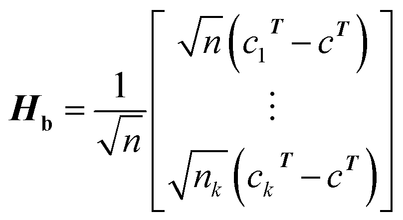and 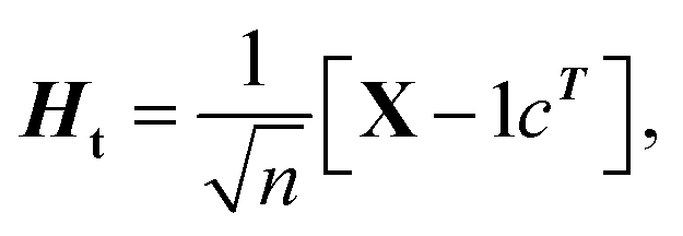H_b and H_t can be calculated.

(2) Convert the singular value decomposition to H_t^T, H_t^T = U∑V^T.

(3) Construct U₁ = [u₁, …, u_r] making sure that u_i(i = 1, 2, …, r) is the r line of matrix U. r is equal to the rank of S_t [r = rank(S_t)]. The total scatter matrix S_t = H_t^TH_t.

(4) Construct making sure that λ_i(i = 1, 2, …, r) is the number of i elements in the diagonal of matrix ∑.

(5) Assuming that Convert the singular value decomposition of matrix B,

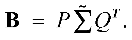
(6) According to 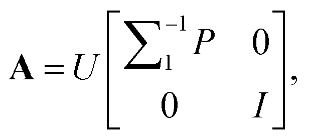matrix A = [a₁, …, a_q, a_q+1, …, a_r] can be calculated.

(7) Collect the column before q of matrix A to structure the transformation matrix G. G = [a₁, …, a_q] and q are equal to the rank of [q = rank(S_b)]. The between-class scatter matrix S_b = H_b^TH_b.

According to the formula Z = XG, a new low dimension data matrix Z is calculated. Then, for the new data X_new, Z_new = X_newG.

2.3 Principal component analysis (PCA)

Principal component analysis (PCA) is one of the most commonly used unsupervised recognition methods. Principal component analysis of a data matrix extracts the dominant patterns in the matrix and represents them as new orthogonal variables (principal components) to display the pattern of similarity in the observations and the variables as points in maps.²⁵

2.4 PLS-DA

PLS-DA consists of a classical PLS regression wherein the response variable is a categorical one expressing the class membership of the statistical units. It is a supervised pattern recognition method and examples of the specific algorithm process can be found in the literature.^26,27

3 Data and calculations

3.1 Data

All the SELDI-TOF MS data comes from the clinical proteomics program of the National Cancer Institute (NCI), U. S. Food and Drug Administration (U. S. FDA). The data were composed of 16 benign tumor serum samples and 100 malignant ovarian tumor serum samples. Each spectrum measured was composed of 15 154 variables (m/z) and their corresponding intensity values. The data can be downloaded freely from http://home.ccr.cancer.gov/ncifdaproteomics/ppatterns.asp.

Fig. 1 shows the SELDI-TOF MS profile of one ovarian tumor example.

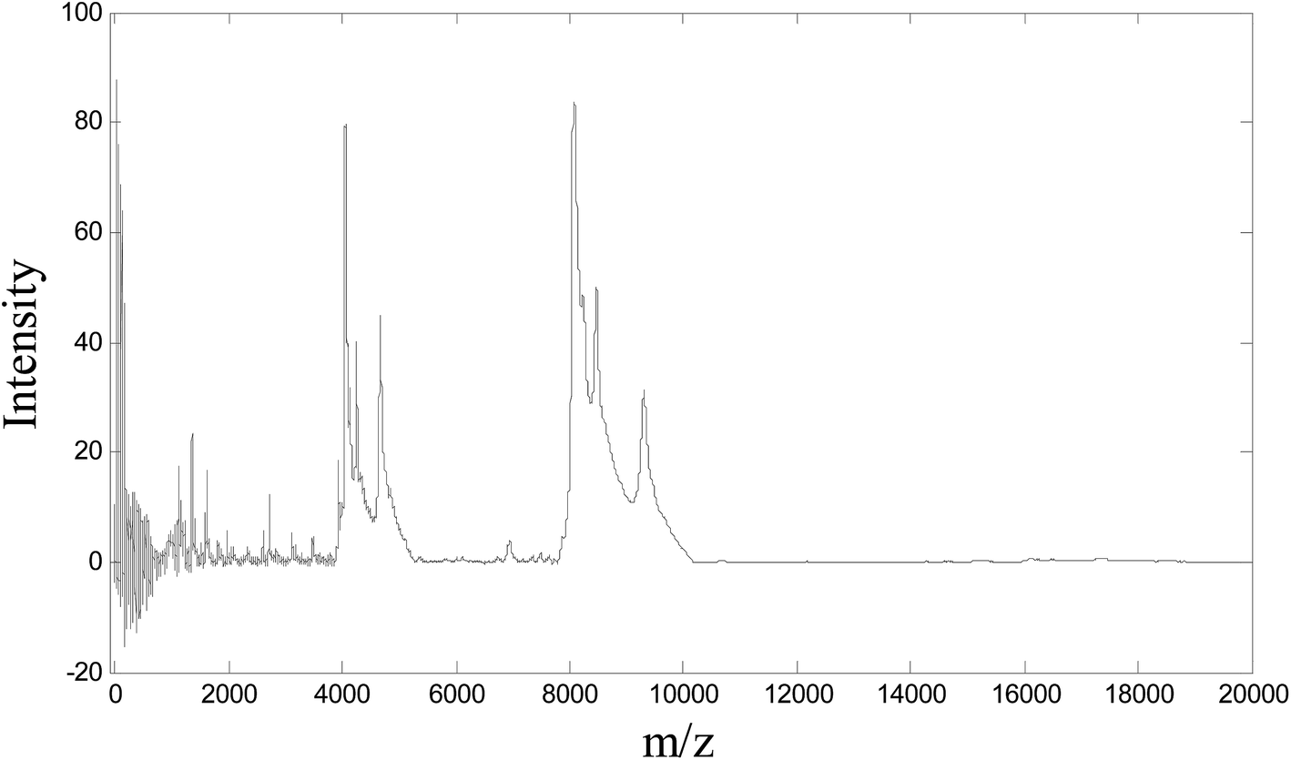Fig. 1 A typical SELDI-TOF MS of one sample.

3.2 Calculations

First, 100 variables were chosen from the 15 154 variables in the original spectra using the variables selection of variance method. Then, the original spectra were replaced with the compressed spectra and introduced to the ULDA, PCA and PLS-DA models. After the variables selection, the models become concise and efficient without redundant information and the calculation speed was also increased.

Then, the sample data were divided into two parts. 50 samples of cancer patients and 8 benign samples were arbitrarily chosen for modeling. The remaining 50 samples of cancer patients and 8 benign samples were used for prediction studies.

Matlab 7.0 was used as the calculation software.

4 Results and discussion

4.1 The results of the ULDA method

Because the number of categories used in this study was two (benign and malignant), only one uncorrelated discriminant vector (UDV) was obtained. Because data visualization in a two-dimensional space was achieved and consequently, the complexity of the model was decreased and the explain ability of the model enhanced. The uncorrelated discriminant vectors of the samples obtained are shown in Fig. 2.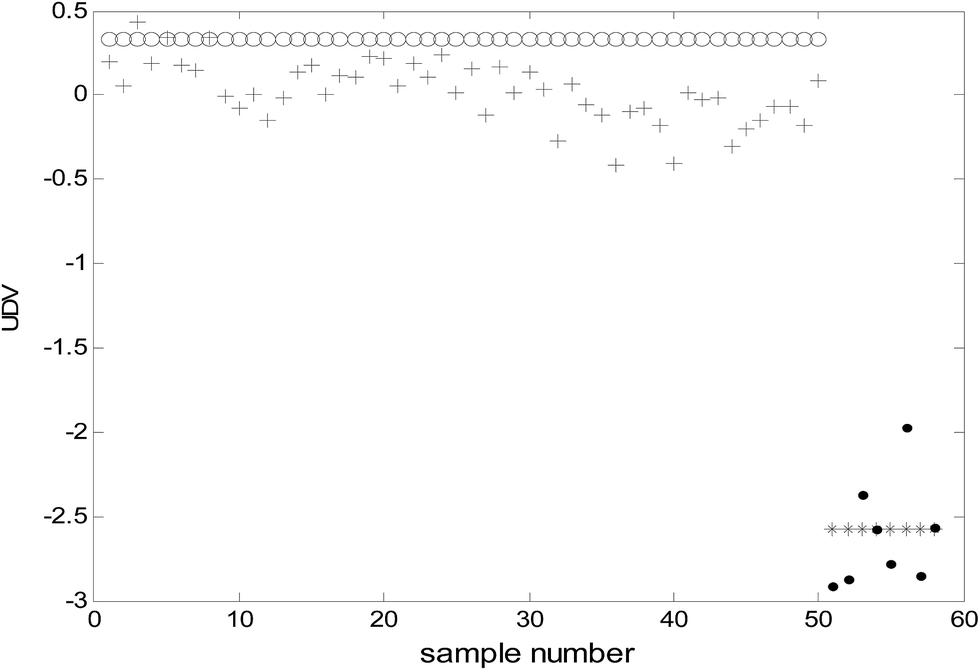

Fig. 2 The uncorrelated discriminant vectors of ULDA (○: malignant samples of modeling; *: benign samples of modeling; +: malignant samples of prediction; ●: benign samples of prediction).

It can be clearly observed from Fig. 2 that the uncorrelated discriminant vectors obtained by ULDA can completely distinguish the cancer samples and benign samples. The samples were classified with 100% sensitivity (percentage of cancer samples correctly identified) and 100% specificity (percentage of benign samples correctly identified) for both the training set and the prediction set.

Because UDV is a linear combination of the original variables (spectra) defined by the coefficients of the transformation vector G, the transformation vector G obtained by ULDA can be looked upon as “loadings” of ULDA. The larger the absolute value of the loadings is, the more important the variable (m/z location) to the classification. A plot of G for the 100 variables is given in Fig. 3, and 7 peak locations with the highest absolute value of G were selected, which can be regarded as potential biomarkers for identifying ovarian cancer samples and benign samples. They were marked up in the transformation vector plot of ULDA with m/z values of 45.7, 45.8, 116.2, 143.4, 4073.6, 8085.3 and 8150.9.

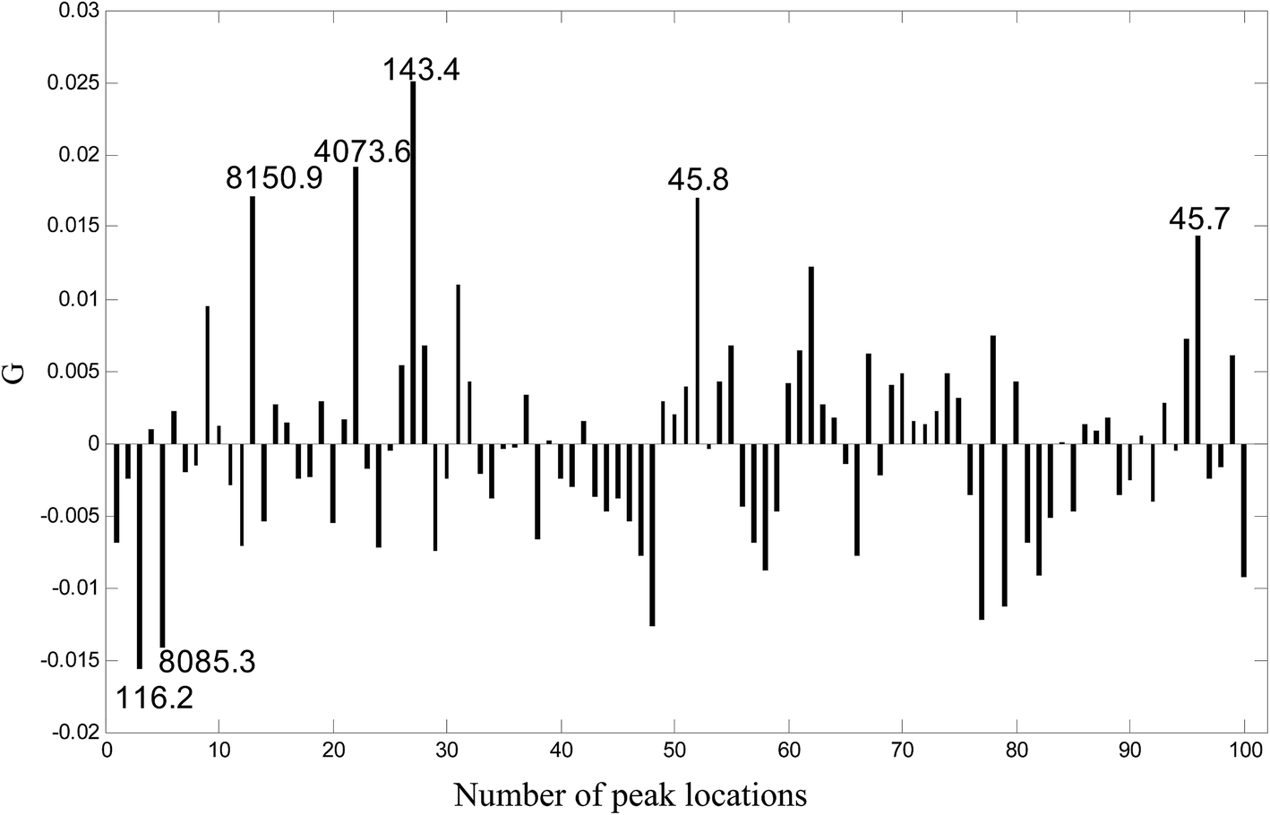Fig. 3 The transformation vector plot for ULDA. Seven peak locations with the highest absolute values of G were selected as potential markers.

To evaluate the performance of the 7 potential biomarkers selected above, new training and prediction matrix were reconstructed from the original ones by collecting the mass spectra only at the 7 m/z locations, which were then analyzed using ULDA. The classification results of the whole data set are presented in Fig. 4. It can be observed that although the UDV values of the two classes were not concentrated as observed in Fig. 2, most of the UDV values for the cancer samples were higher than −1.40 and the UDV values for the benign samples were below −1.40. At the watershed of −1.40, the ULDA obtained 97% (97/100) sensitivity and 100% (16/16) specificity. The results revealed that the proposed method is promising for the selection of potential biomarkers. Biomarker screening is very important in proteomics studies. It should be pointed out that in this study the potential biomarkers selected were m/z locations but not real proteins, they are highly informative for tumor identification and contribute to further study on proteomic biomarkers.

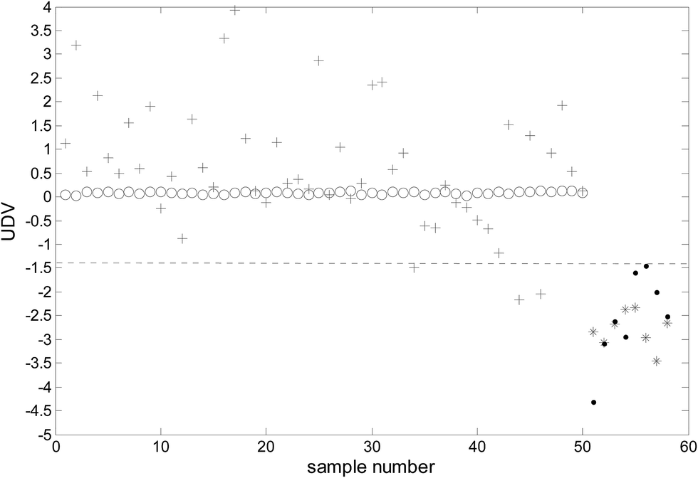Fig. 4 The classification results of ULDA using the seven m/z positions (○: malignant samples of modeling; *: benign samples of modeling; +: malignant samples of prediction; ●: benign samples of prediction).

In Conclusion, the proposed strategy based on ULDA combined with variance analysis of serum SELDI-TOF MS is promising for malignant and benign tumor identification.

4.2 The results of the PCA and PLS-DA methods

As an unsupervised recognition method, the classification results for malignant and benign groups in the first two principal component space (PC1 and PC2) are shown in Fig. 5. In Fig. 5, it can be clearly observed from the component scores that the malignant group and benign group cannot be completely separated due to seriously overlapping of the scores. Even though more principal components were used for the data, the classification results were not significantly improved. In this study, the number of principal factors in the PLS-DA modeling was set at 15 through optimization. As an supervised recognition method, the malignant group was marked as [1,0] and the benign group was marked as [0,1] in advance. The predicted results obtained using PLS-DA are given in Fig. 6. From Fig. 6, it was found that in the malignant group, 9 of the 50 samples were wrongly classified. In the benign group, all the samples were classified correctly. The samples in the prediction set were classified with 82% sensitivity and 100% specificity.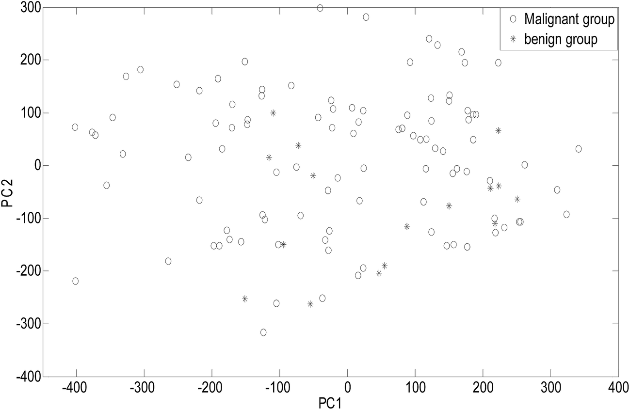

Fig. 5 The PC scores plot.

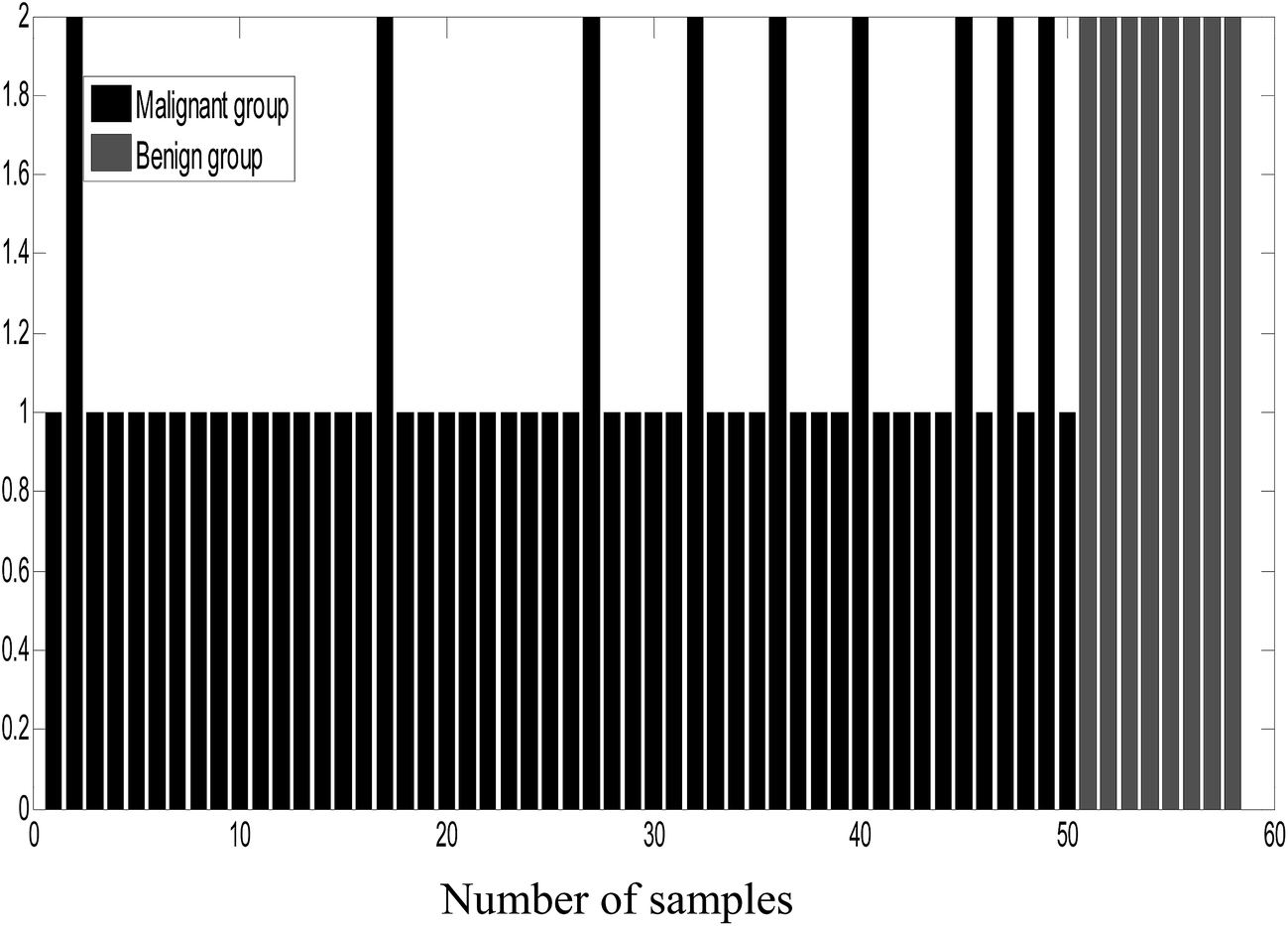Fig. 6 The column diagram of PLS-DA classification.

After comprehensive analysis of the abovementioned results, it can be concluded that the ULDA method was superior to the PCA and PLS-DA methods when applied to classifying malignant and benign tumor serum samples.

In general, PCA and PLS-DA are commonly used methods for feature extraction. However, PCA and PLS-DA are sometimes not very efficient for proteomic data analysis, as discussed in the literature.²⁸ A lot of dimension reduction of the learning task can be completed by PCA, but its comprehension of the characteristics is very poor; even a simple linear combination of the characteristics will also make it difficult to understand. PLS-DA considers the information obtained from the sample classification in the feature selection procedure. Nevertheless, PLS-DA is essentially a feature transformation approach, the new variables are some type of combination of the original variables. The variables with large variance or high covariance can affect the results, although those variables contain little or even no information contributing to the discrimination of samples, which may result in the loss of optimal features in some situations.^29,30

The ULDA algorithm considers no correlation between column vectors in the transformation matrix; therefore, it can reduce the data redundancy after dimension reduction. UDVs with the biggest discriminant ability are extracted and vectors are not related to each other. In this case, ULDA maximizes the degree of different category samples.³¹

5 Conclusions

The method of ULDA algorithm combined with variables selection applied to the identification of SELDI-TOF MS serum peptide profiles of malignant and benign tumor samples obtained good results. In addition, specific peaks (m/z locations) as potential biomarkers were chosen. The proposed method used in this study is promising for malignant and benign ovarian tumor identification and the selection of potential biomarkers.

Acknowledgements

This study is supported by the National Natural Science Foundation of China (No. 21305043), the Beijing Natural Science Foundation (No. 7142102) and the Fundamental Research Funds for the Central Universities (No. 2014ZD38).

References

1. R. Madsen, T. Lundstedt and J. Trygg, Anal. Chim. Acta, 2010, 659(1–2), 23–33.
2. H. Junker, S. Venz, U. Zimmermann, A. Thiele, C. Scharf and R. Walther, PLoS One, 2011, 6(7), e21867.
3. G. Bellisola and C. Sorio, Am. J. Cancer Res., 2012, 2(1), 1–21.
4. L. Liu, D. Cozzolino, W. U. Cynkar, R. G. Dambergs, L. Janik, B. K. O'Neill, C. B. Colby and M. Gishen, Food Chem., 2008, 106, 781–786.
5. L. Louw, K. Roux, A. Tredoux, O. Tomic, T. Naes, H. H. Nieuwoudt and P. van Rensburg, J. Agric. Food Chem., 2009, 57(7), 2623–2632.
6. E. Sikorska, T. Gorecki, I. V. Khmelinskii, M. Sikorski and D. de Keukeleire, J. Inst. Brew., 2004, 110, 267–275.
7. H. Abdi and L. J. Williams, Wiley Interdisciplinary Reviews: Computational Statistics, 2010, 2(4), 433–459.
8. M. Steidel, R. Fragnoud, M. Guillotte, C. Roesch, S. Michel, T. Meunier, G. Paranhos-Baccala and G. Gervasi, J. Med. Virol., 2012, 84(3), 490–499.
9. A. Xue, R. C. Gandy, L. Chung, R. C. Baxter and R. C. Smith, Pancreatology, 2012, 12(2), 124–129.
10. Q. X. Yang, L. X. Zhang, L. X. Wang and H. B. Xiao, Chemom. Intell. Lab. Syst., 2012, 116, 1–8.
11. L. Norgaard, A. Saudland, J. Wagner, J. P. Nielsen, L. Munck and S. B. Engelsen, Appl. Spectrosc., 2000, 54, 413–419.
12. R. F. Kokaly and R. N. Clark, Rem. Sens. Environ., 1999, 67, 267–287.
13. W. S. Cai, Y. K. Li and X. G. Shao, Chemom. Intell. Lab. Syst., 2008, 90, 188–194.
14. Y. K. Li and J. Jing, Anal. Methods, 2012, 4, 254–258.
15. R. Leardi and A. L. Gonzalez, Chemom. Intell. Lab. Syst., 1998, 41, 195–207.
16. X. L. Chu, H. F. Yuan and W. Z. Lu, Progress in Chemistry, 2004, 16, 528–542.
17. R. F. Shan, W. S. Cai and X. G. Shao, Chemom. Intell. Lab. Syst., 2014, 131, 31–36.
18. Z. Jin, J. Y. Yang, Z. S. Hu and Z. Lou, Pattern Recogn., 2001, 34, 1405–1416.
19. Z. Jin, J. Y. Yang, Z. M. Tang and Z. S. Hu, Pattern Recogn., 2001, 34, 2041–2047.
20. J. Ye, J. Mach. Learn. Res., 2005, 6, 483–502.
21. D. Q. Dai and P. C. Yuen, Pattern Recogn., 2003, 36, 845–847.
22. J. H. Friedman, J. Am. Stat. Assoc., 1989, 84, 165–175.
23. L. Chen, H. M. Liao, M. Ko, J. Lin and G. Yu, Pattern Recogn., 2000, 33, 1713–1726.
24. Y. Z. Liang and Q. S. Xu, Complex system analysis instrument, Chemical industry Press, Beijing, 2012, pp. 525–536.
25. S. Lopez-Urena, M. Beneito-Cambra, R. M. Donat-Beneito and G. Ramis-Ramos, Anal. Methods, 2015, 7, 3080–3088.
26. H. Wold, Encyclopedia of statistical science, 1985, vol. 6, pp. 581–591.
27. S. M. van Ruth, B. Villegas, W. Akkermans, M. Rozijn, H. van der Kamp and A. H. Koot, Food Chem., 2010, 118, 948–955.
28. R. Rousseau, B. Govaerts, M. Verleysen and B. Boulanger, Chemom. Intell. Lab. Syst., 2008, 91, 54–66.
29. S. S. Heinzmann, I. J. Brown, Q. Chan, M. Bictash, M. E. Dumas, S. Kochhar, J. Stamler, E. Holmes, P. Elliott and J. K. Nicholson, Am. J. Clin. Nutr., 2010, 92, 436–443.
30. M. M. Zeng, Y. Z. Liang, H. D. Li, B. Wang and X. Chen, Anal. Methods, 2011, 3, 438–445.
31. D. L. Yuan, Y. Z. Liang, L. Z. Yi, Q. S. Xu and O. M. Kvalheim, Chemom. Intell. Lab. Syst., 2008, 93, 70–79.

---