DOI:
10.1039/C5SM01507C
(Paper)
Soft Matter, 2015,
11, 7402-7411
Nonlinear electro-osmosis of dilute non-adsorbing polymer solutions with low ionic strength
Received
18th June 2015
, Accepted 4th August 2015
First published on 4th August 2015
Abstract
Nonlinear electro-osmotic behaviour of dilute non-adsorbing polymer solutions with low salinity is investigated using Brownian dynamics simulations and a kinetic theory. In the Brownian simulations, the hydrodynamic interaction between the polymers and a no-slip wall is considered using the Rotne–Prager approximation of the Blake tensor. In a plug flow under a sufficiently strong applied electric field, the polymer migrates toward the bulk, forming a depletion layer thicker than the equilibrium one. Consequently, the electro-osmotic mobility increases nonlinearly with increasing electric field and becomes saturated. This nonlinear mobility does not depend qualitatively on the details of the rheological properties of the polymer solution. Analytical calculations using the kinetic theory for the same system quantitatively reproduce the results of the Brownian dynamics simulation well.
1 Introduction
Electro-osmosis is observed widely in many systems such as colloids, porous materials, and biomembranes. It characterises the properties of interfaces between solids and electrolyte solutions.1,2 Interest in the applications of electro-osmosis has been growing recently. For instance, it is used to pump fluids in microfluidic devices, as it is more easily implemented than pressure-driven flow.3 Its application to electrical power conversion in chemical engineering is also very fascinating.4,5 When the electrokinetic properties of a surface are characterised by a zeta potential, the Smoluchowski equation is often employed in conjunction with measurements of the electro-osmotic or electrophoretic mobilities. However, the validity of this equation should be considered more seriously. It is derived from the Poisson–Boltzmann equation and Newton's constitutive equation for viscous fluids. The zeta potential is defined as the electrostatic potential at the plane where a no-slip boundary condition is assumed. When these equations cannot be validated, the Smoluchowski equation is also questionable. The Poisson–Boltzmann equation, the simple hydrodynamic equations, or both sometimes do not work well for a strong coupling double layer,6 inhomogeneity of viscosity and dielectric constant near the interface,7,8 and non-Newtonian fluids,9–12 for example.
To control the electrokinetic properties of charged capillaries, the structures of liquid interfaces in contact with charged surfaces are modified by grafting or adding polymers.13 In capillary electrophoresis, for example, the electro-osmotic flow is reduced by grafted polymers on the interfaces. Several studies of surfaces with end-grafted charged and uncharged polymers have also been reported.14–19 Under a weak applied electric field, the grafted polymer remains in the equilibrium configuration, and the resultant electro-osmotic velocity behaves linearly with respect to the electric field. To measure the mobility of such a surface, the hydrodynamic screening and anomalous charge distributions due to the grafted polymers are important.14–19 When a sufficiently strong electric field is applied, the polymers are deformed by the flow and the electric field; thus, the electro-osmotic velocity becomes nonlinear.16 Note that the end-grafted polymers cannot migrate toward the bulk, as one of the ends is fixed on the surfaces.
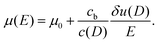
When we add polymers to solutions, a depletion or adsorption layer is often formed near a solid wall, as well as diffusive layers of ions in equilibrium states. The interaction between the polymers and the wall determines whether the polymers are depleted from or adhere to the surfaces. The thickness of the depletion or adsorption layer is of the same order as the gyration length of the polymers. When polymers adhere to the wall, the viscosity near the wall becomes large, so the electro-osmotic mobility is strongly suppressed.20 Moreover, it is known that an adsorption layer of charged polymers can change the sign of mobility.7,21–24 The curvature of the surface also modulates the surface charge density and even increases the mobility beyond the suppression caused by viscosity enhancement.20
Electro-osmosis of a non-adsorbing polymer solution has been analysed in terms of two length scales: the equilibrium depletion length δ0 and the Debye length λ.7,25 In the depletion layer, the viscosity is estimated to be approximately the same as that of the pure solvent, and it is smaller than the solution viscosity in the bulk. When the Debye length is smaller than the depletion length, the electro-osmotic mobility is larger than that estimated from the bulk value of viscosity. Typically, for 10 mM electrolyte solutions, one has λ ≈ 3 nm and δ0 ≈ 100 nm. In such a case,26–28 an electro-osmotic flow with a high shear rate is localised at a distance λ from the wall. Thus, the electro-osmotic flow profile and resultant electro-osmotic mobility are almost independent of the polymers. Such behaviours are experimentally observed in solutions of carboxymethyl cellulose with urea.27 On the other hand, in the solutions of small polymers with low salinity (typically for 0.1 mM electrolyte solutions, λ ≈ 30 nm and δ0 ≈ 5 nm), the electro-osmotic mobility is suppressed by the polymeric stress.25
When a sufficiently strong electric field is applied, the electro-osmosis of a polymer solution shows nonlinear behaviours.27,29 These nonlinearities are theoretically analysed by models of uniform non-Newtonian shear-thinning fluids.9–12 Assuming that polymers remain in the interfacial layers and viscosity depends on the local shear rate, as in power-law fluids, their phenomenological parameters differ from those in the bulk, as the concentration in the interfacial layers differs from the bulk concentration.27 Thus, the understanding of nonlinear electro-osmosis remains phenomenological. Furthermore, when shear flow is applied to polymer solutions near a wall, it is experimentally and theoretically confirmed that cross-stream migration is induced toward the bulk.30–32 The concentration profiles of the polymer near the wall have been calculated, and the depletion length dynamically grows tenfold larger than the gyration radius.31 However, these hydrodynamic effects in the electrokinetics have not been studied to date, to the best of our knowledge.
In this context, this paper discusses another origin of nonlinearity, which is induced by hydrodynamic interaction between the polymer and the wall, considering mainly situations where δ0 ≪ λ. For this purpose, this paper is organised as follows. Section 2 presents a toy model of nonlinear electro-osmosis of dilute polymer solutions. Section 3 describes the Brownian dynamics simulation, and Section 4 presents the results of the simulation. In Section 5, we discuss an analytical approach to nonlinear electro-osmosis by using the kinetic theory of cross-stream migration.31 Section 6 outlines the main conclusions.
2 Toy model
First, we propose a toy model for electro-osmosis of polymer solutions. A dilute solution of non-adsorbing polymers is considered. The viscosity of the solution is given bywhere η0 is the viscosity of the pure solvent, and ηsp is the specific viscosity of the solution. The gyration length of the polymers is defined as δ0, which is of the same order as the equilibrium depletion length. It is assumed that the polymers have δ0 ≈ 100 nm. Ions are also dissolved in the solution with the Debye length λ. When well-deionised water is considered, the Debye length is on the order of λ ≈ 103 nm, although such salt-free water is rarely realised owing to the spontaneous dissolution of carbon dioxides. The interfacial structure near a charged surface is characterised by λ and δ0. When an external electric field is applied, a shear flow is imposed locally within a distance λ from the wall, and the resultant shear rate is| |  | (2) |
where μ0 is the electro-osmotic mobility of the pure solvent and is typically estimated as μ0 ≈ 10−8 m2 (V s)−1. According to studies of cross-stream migration in uniform shear flow,31 the depletion layer thickness depends on the shear rate,| | δ ≈ δ0(τ![[small gamma, Greek, dot above]](https://www.rsc.org/images/entities/i_char_e0a2.gif) )2, )2, | (3) |
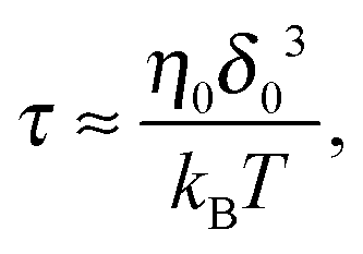
where τ is the characteristic relaxation time of the polymers,| |  | (4) |
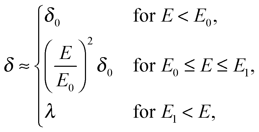
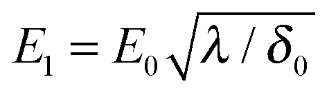
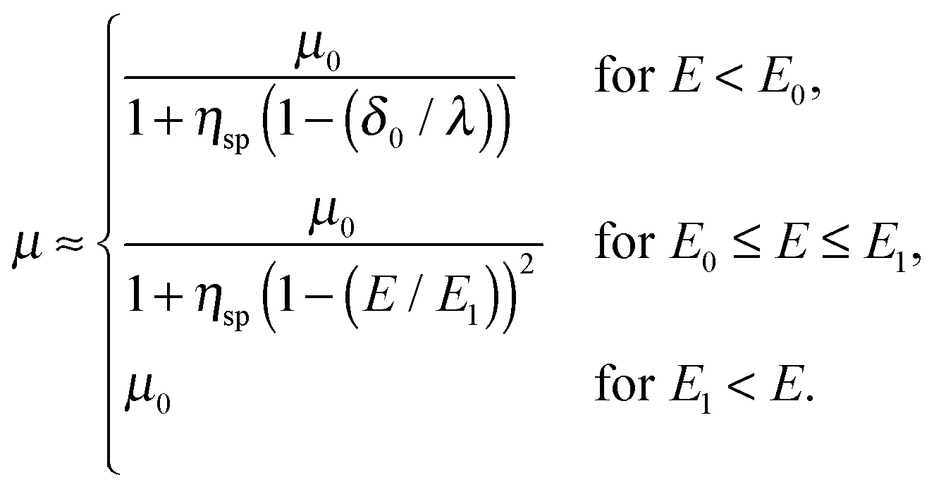
where kBT is the thermal energy, and is typically 10−4 s at room temperature. Using eqn (2) and (3), the depletion length in the presence of the applied electric field E can be expressed as| |  | (5) |
where E0 = λ/τμ0, and  . Here, for simplicity, we assume that the depletion length does not exceed the Debye length. The effective viscosity in the double layer is given by
| | 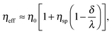 | (6) |
and the nonlinear mobility can be estimated as μ ≈ μ0(η0/ηeff). Therefore, the mobility is obtained as| |  | (7) |
Fig. 1(a) schematically shows the thickness of the depletion layer as a function of the electric field strength. Fig. 1(b) shows the nonlinear electro-osmotic mobility. The mobility increases and is saturated with increasing electric field. The threshold electric field E0 is typically 103 V m−1, which is experimentally accessible.
 |
| | Fig. 1 (a) Depletion length as a function of the applied electric field. (b) Electro-osmotic mobility as a function of the applied electric field. | |
3 Model for simulation
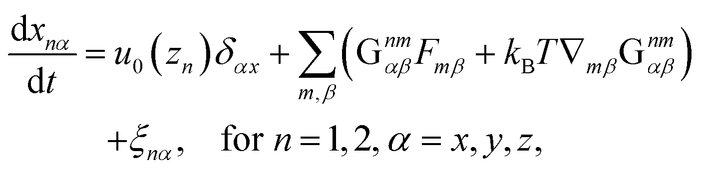
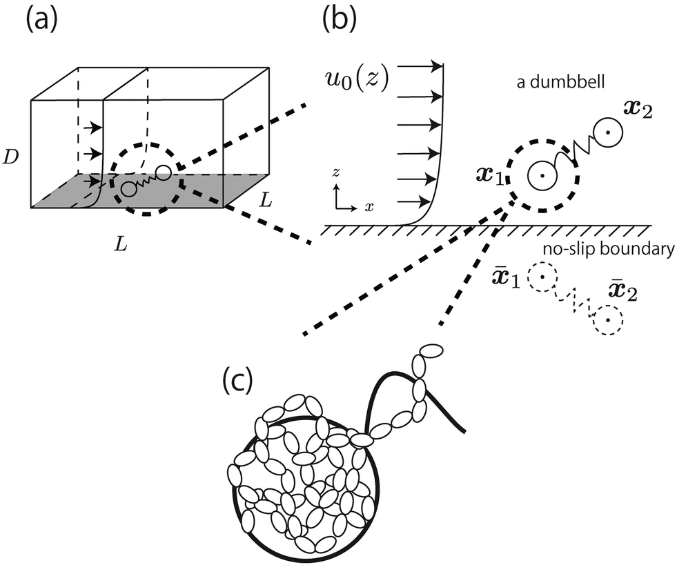
In this section, our method of Brownian dynamics simulation is described. As shown in Fig. 2(a), a dumbbell is simulated in an electrolyte solution with a no-slip boundary at z = 0. The dumbbell behaves like a dilute solution. The solvent is described as a continuum fluid with the viscosity η0 and fills the upper half of the space (z > 0). Electrolytes are also treated implicitly with the Debye length λ = κ−1. The dumbbell has two beads whose hydrodynamic radii are a, and each bead consists of many monomeric units of the polymer [see Fig. 2(c)]. The positions of the beads are represented by x1 and x2 [see Fig. 2(b)]. Then we solve the overdamped Langevin equations33 given by| |  | (8) |
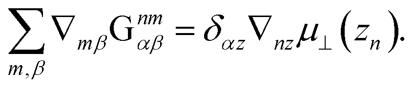
where Xnα is the α component of vector Xn. Furthermore, u0(z) is the external plug flow, ∇nα = ∂/∂xnα, G is the mobility tensor, Fn = −∇nU is the force exerted on the nth bead, and U is the interaction energy given as a function of xn. ξn is the thermal noise which satisfies the fluctuation–dissipation relation as| | | 〈ξnα(t)ξmβ(t′)〉 = 2kBTGnmαβδ(t − t′). | (9) |
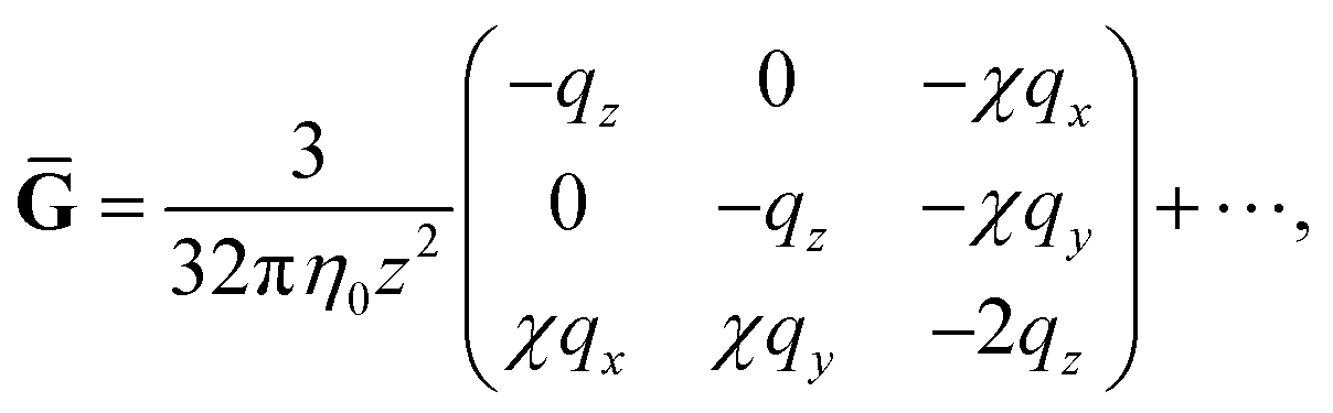
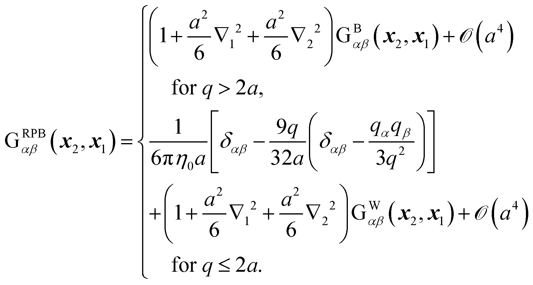
To include the effects of the no-slip boundary, the Rotne–Prager approximation for the Blake tensor34 is used as the mobility tensor for distinct particles (n ≠ m),35,36 although it is valid only for particles separated by a large distance. In this study, we neglect lubrication corrections for nearby particles.37 The Blake tensor for the velocity at x2 induced by a point force at x1 with the no-slip boundary at z = 0 is given by the Oseen tensor and the coupling fluid–wall tensor as34| | | GBαβ(x2,x1) = Sαβ(q) + GWαβ(x2,x1), | (10) |
where q = x2 − x1, R = x2 − ![[x with combining macron]](https://www.rsc.org/images/entities/b_i_char_0078_0304.gif) 1, and 1 is the mirror image of x1 with respect to the plane z = 0 [see Fig. 2(b)]. The Oseen tensor is given by
1, and 1 is the mirror image of x1 with respect to the plane z = 0 [see Fig. 2(b)]. The Oseen tensor is given by| |  | (11) |
where q is the magnitude of q. The second term in eqn (10) is| | | GWαβ(x2,x1) = −Sαβ(R) + z12(1 − 2δβz)∇R2Sαβ(R) − 2z1(1 − 2δβz)Sαz,β(R), | (12) |
where| | | Sαβ,γ(q) = ∇qγSαβ(q), | (13) |
and ∇qγ = ∂/∂qγ. The Rotne–Prager approximation of the Blake tensor is given by6,35–38| |  | (14) |
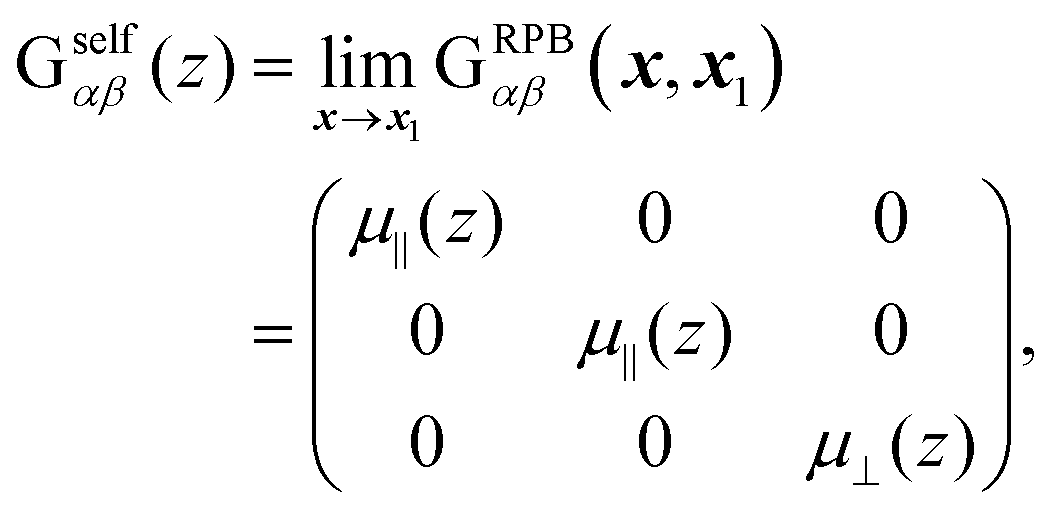
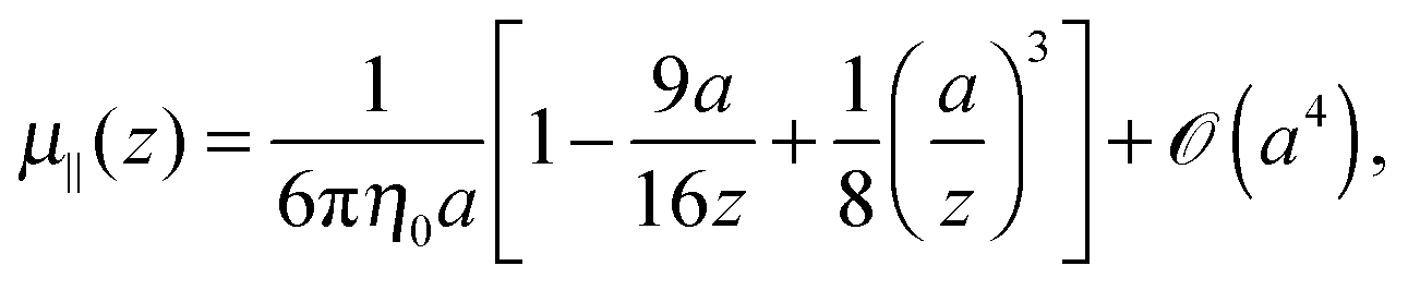
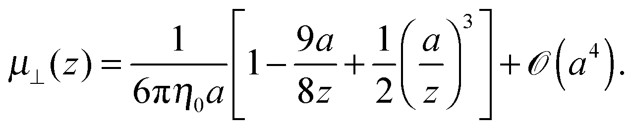
The mobility tensor for the self-part is given by6,35–38| | 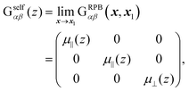 | (15) |
where| | 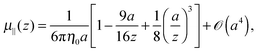 | (16) |
| |  | (17) |
Finally we obtain the mobility tensor as| | | Gnmαβ = δnmGselfαβ(zn) + (1 − δnm)GRPBαβ(xn,xm). | (18) |
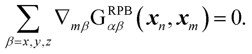
The non-uniform mobility term in eqn (8) can be simplified within the Rotne–Prager approximation of the Blake tensor because the following relation holds:| |  | (19) |
Thus, the non-uniform mobility term is rewritten as| |  | (20) |
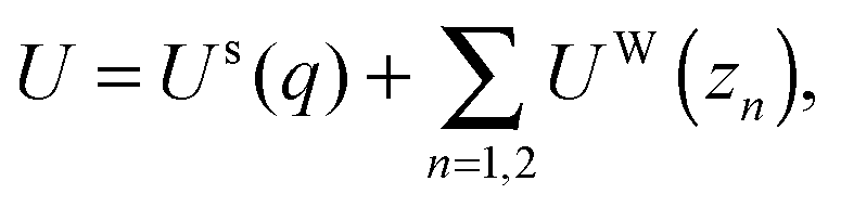
The interaction energy includes the spring and bead–wall interaction given by| |  | (21) |
where Us is the spring energy,| |  | (22) |
where a FENE dumbbell is a finitely extensible nonlinear elastic dumbbell, and the parameter b = Hq02/kBT is defined for convenience. Uw is the bead–wall interaction,39 which is purely repulsive:| |  | (23) |
Eqn (8) is solved numerically. A reflection boundary condition is set at z = D. When the centre of the dumbbell crosses the boundary, the z coordinates of each bead are transformed from z to 2D − z. In the lateral directions, periodic boundary conditions are imposed. The size of the lateral directions is L × L.
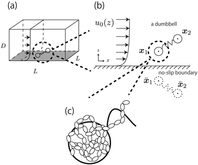 |
| | Fig. 2 (a) Dumbbell in the simulated box with L × L × D. A periodic boundary condition is imposed at the x–y plane. (b) An x–z projection of the dumbbell in the electro-osmotic flow. (c) Enlarged illustration of the bead in the dumbbell. It is composed of many monomeric units of the polymers. | |
4 Results of simulation
The concentration and velocity profiles are calculated as| | 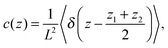 | (24) |
and| | 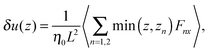 | (25) |
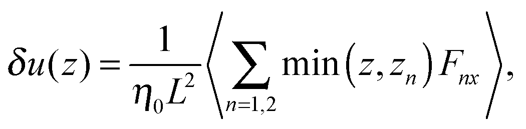
where δ(z) is the delta function, δu(z) = u(z) − u0(z) is the increase in velocity due to polymeric stress, and 〈⋯〉 is the statistical average in the steady state. Eqn (25) is derived in Appendix A.
For a surface with a small zeta potential compared to kBT/e, where e is the elementary charge, the imposed electro-osmotic flow u0(z) is given by
| | | u0(z) = μ0E(1 − e−κz), | (26) |
where
μ0 is the electro-osmotic mobility in the pure solvent, and
E is the applied electric field.
2Eqn (8) is rewritten in a dimensionless form with the length scale

and time scale
τ = 6π
η0a/4
H. Different types of dumbbells are simulated using the parameters listed in
Table 1.
Table 1 Simulation parameters. Nt is the number of total steps, Ni is the number of interval steps for observation, Nm is the number of sampling for each parameter set, and Δτ is the increase in time
| |
Hookian |
FENE b = 600 |
FENE b = 50 |
|
N
t
|
5 × 10¹⁰ |
5 × 10¹⁰ |
25 × 1010 |
|
N
i
|
5 × 10³ |
5 × 10³ |
25 × 103 |
|
N
m
|
3 |
3 |
5 |
| Δτ |
0.01 |
0.0025 |
0.0001 |
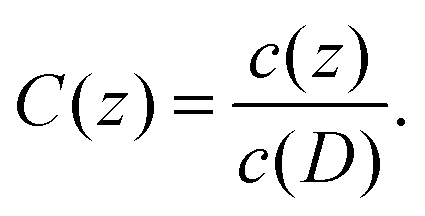
Note that the simulated systems are treated as dilute systems, and the linearity with respect to the bulk polymer concentration is preserved. After sample averaging, we obtain the concentration at the upper boundary c(D), which deviates slightly from (L2D)−1 because of the inhomogeneity near the surface. Hereafter, we define the normalised concentration as
| |  | (27) |
The velocity increment
δu(
z), as well as the concentration profile, is linear with respect to
c(
D). For convenience, we set a characteristic concentration
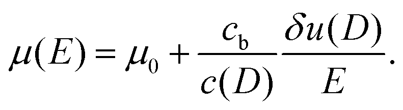
cb = 0.1
δ0−3, and the nonlinear electro-osmotic mobility is defined as
| |  | (28) |
The top boundary is placed at
D = 100
δ0, the lateral size is set to
L = 1000
δ0, and the Debye length is set to
λ =
κ−1 = 10
δ0. We also set
w = 3
kBT and define a hydrodynamic parameter
h* as
31| | 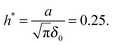 | (29) |
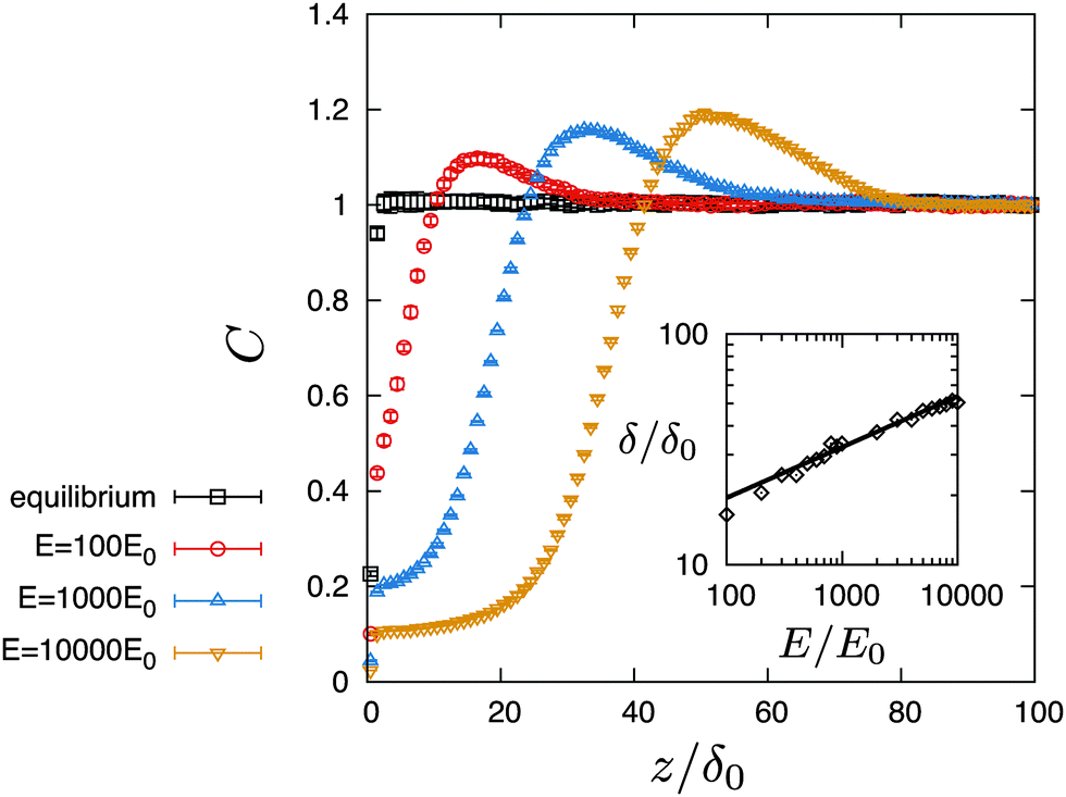
Fig. 3 shows the steady-state profiles of the Hookian dumbbell concentration as functions of the distance from the wall. In the equilibrium state of
E = 0, the profile shows a depletion layer whose width is of the same order as the gyration length
δ0. When the applied electric field is increased further, the depletion layer becomes larger than the equilibrium one, and a peak is formed. The inset in
Fig. 3 shows the depletion length as a function of the applied field. The depletion length is defined by the position of the concentration peak. It shows power-law behaviour with an exponent of 0.22, which is much smaller than that of 2.0 for a uniform shear flow.
31 The value of concentration at the peak also increases as the electric field increases.
 |
| | Fig. 3 Concentration profiles of Hookian dumbbells under various applied electric fields. Inset shows the depletion length as a function of the applied field. The points are obtained by the Brownian dynamics simulation, and the line is fitted by δ/δ0 = A(E/E0)B, where A = 7.08, and B = 0.22. | |
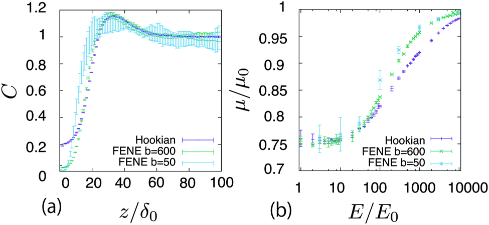
The results given above are for the Hookian dumbbell which is infinitely extensible with shear deformation. To consider more realistic polymers, the finitely extensible nonlinear elastic (FENE) dumbbell is simulated. Fig. 4(a) shows the concentration profiles at E = 1000E0. Interestingly, one-peak behaviour is also observed in the FENE dumbbells. For the Hookian dumbbell, the concentration near the surface remains finite. On the other hand, for the FENE dumbbells, the concentrations near the surface are negligibly small. Fig. 4(b) plots the electro-osmotic mobilities with respect to the applied electric field. The resultant electro-osmosis clearly increases nonlinearly with respect to the applied electric field. When the applied field becomes stronger, the mobility increases and is saturated, similar to that in the toy model. The two types of dumbbells have different rheological properties in the bulk,40–42 so this nonlinearity is not due to the rheological properties of the dumbbells. On the other hand, the mobility is almost constant for E ≲ 10E0, and this threshold of linearity is larger than E0, which is predicted by the toy model. Likewise, saturation is observed when E ≈ 104E0, which is larger than E1.
 |
| | Fig. 4 (a) Concentration profiles of the polymers at E = 1000E0 in different types of dumbbells. (b) Nonlinear electro-osmotic mobility with respect to E. | |
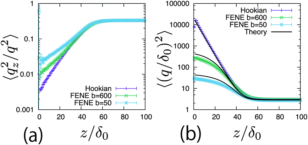
To clarify the difference in the profiles near the surface, 〈q2〉 and 〈qz2/q2〉 are plotted with respect to the distance from the surface. Fig. 5(a) shows the profiles of 〈qz2/q2〉. In the bulk, they approach 1/3, which means that the dumbbells are distributed isotropically. Near the surface, the polymers are inclined by the shear flow. The Hookian dumbbell has the largest angle between the z axis and the dumbbell direction. Fig. 5(b) plots the profiles of 〈q2〉. In the bulk, they approach 3δ0, which is their equilibrium value. Near the surface, they become larger because the polymers are elongated by the shear flow. For the FENE dumbbells, saturation of the dumbbell length is observed. These behaviours differ greatly from the minor differences in the concentration profiles.
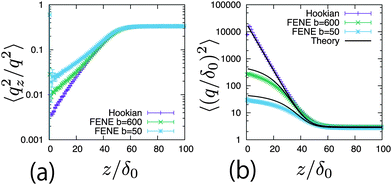 |
| | Fig. 5 (a) Profiles of 〈qz2/q2〉 at E = 1000E0 in different types of dumbbells. (b) Profiles of 〈(q/δ0)2〉 at E = 1000E0 in different types of dumbbells. Curved lines are calculated using eqn (62) and (71). | |
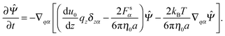
5 Kinetic theory
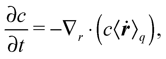
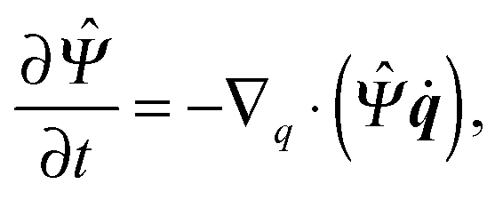
In this section, a kinetic theory for a dumbbell is developed on the basis of the Ma–Graham theory.31 The probability function Ψ(x1,x2,t) obeys the continuity equation| |  | (30) |
where ẋn is the flux velocity given by43| |  | (31) |
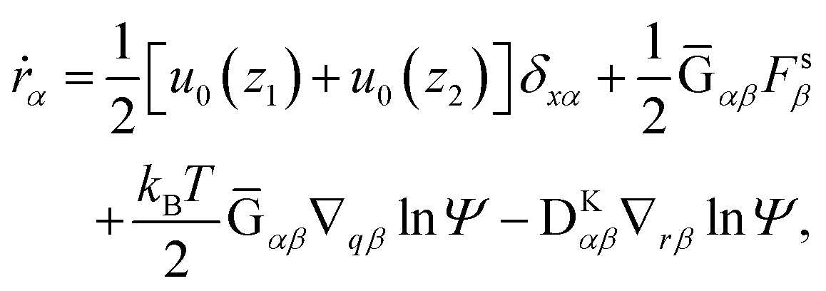
In the kinetic model, the beads are treated as point-like particles. Thus, the mobility tensor is obtained by using GB instead of GRPB for both the self and distinct parts. The continuity equation can be rewritten using q and r as| |  | (32) |
where r = (x1 + x2)/2 is the centre of the mass of the dumbbell. We also define ∇1 and ∇2 as| |  | (33) |
| |  | (34) |
Then, the probability function is also regarded as a function of r and q. Here we neglect the interaction between the wall and the beads. The flux velocities for r and q are obtained as| | 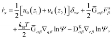 | (35) |
| |  | (36) |
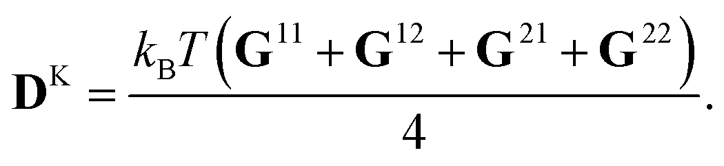
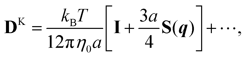
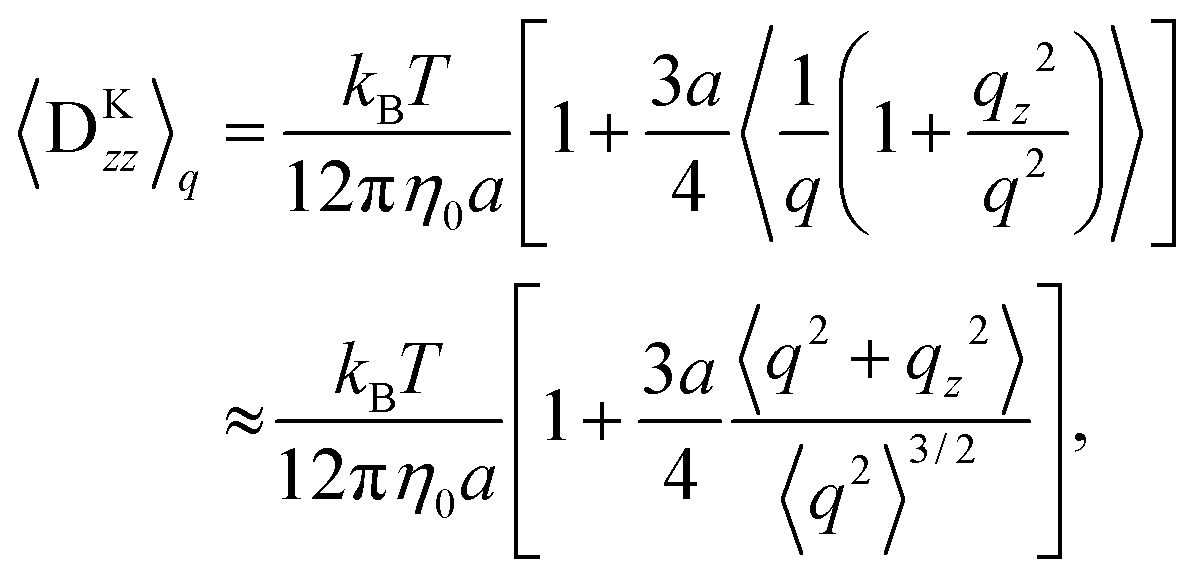
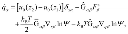
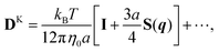
where Fs = −∇1Us is the spring force, and DK is the Kirkwood diffusion tensor, which characterises the diffusivity of macromolecules and is given by| | 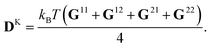 | (37) |
Ḡ and Ĝ are variants of the mobility tensors defined as| | | Ḡ = G11 − G12 + G21 − G22, | (38) |
| | | Ĝ = G11 − G12 − G21 + G22. | (39) |
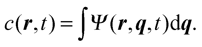
The concentration field c(r,t) can be obtained by integrating the probability function with respect to the spring coordinate. It is given by| |  | (40) |
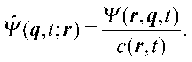
We also define the probability function only for the spring coordinate as| | 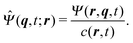 | (41) |
These new fields satisfy the continuity conditions, such that| |  | (42) |
| |  | (43) |
where 〈⋯〉q represents the average with the spring coordinate:| |  | (44) |
For the limit of q ≪ r, Ḡ and DK can be expanded using r. Keeping only the leading term, we obtain| | 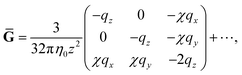 | (45) |
| |  | (46) |
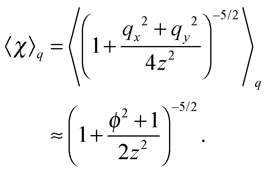
where| | 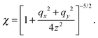 | (47) |
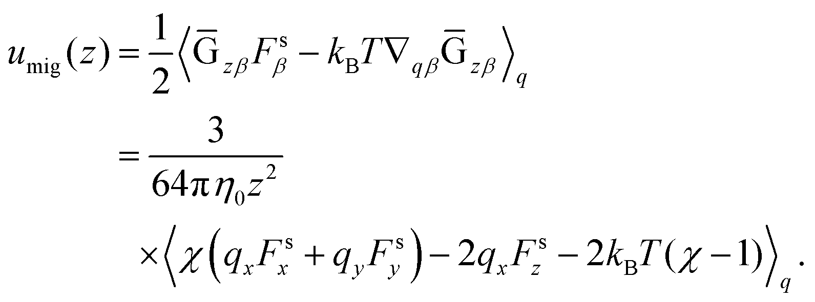
Note that the approximation is more accurate than that in a previous study31 as that study considered only χ ≈ 1, which is not satisfied near the surface. With the approximation, eqn (36) is averaged by ![[capital Psi, Greek, circumflex]](https://www.rsc.org/images/entities/i_char_e0b0.gif) , and finally we obtain the concentration flux for the z direction as
, and finally we obtain the concentration flux for the z direction as| | 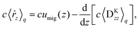 | (48) |
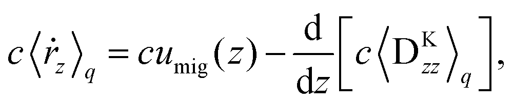
where| |  | (49) |
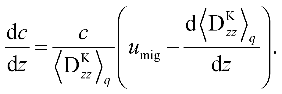
Eqn (48) indicates two opposite fluxes of the polymers due to the external flow field. One is the migration flux from the wall toward the bulk and originates from the hydrodynamic interaction between the wall and the force dipoles.31 The other is the diffusion flux from the bulk to the surface wall and is not found for polymers in uniform shear flows.31 Note that the second flux includes not only the ordinary diffusion flux 〈DKzz〉q∇rzc, but also the diffusion flux due to q inhomogeneity, c∇rz〈DKzz〉q. When the external shear flow is uniform, the second flux vanishes, and the depletion length is proportional to the square of the shear rate, as the migration velocity is proportional to the normal stress difference.31 In a plug flow, the diffusion flux suppresses the growth of the depletion layer, and this behaviour may explain why the exponent of the depletion length is much smaller than 2.0 in a uniform shear flow. In the steady states of electro-osmosis, the total flux in eqn (48) becomes zero; thus,| | 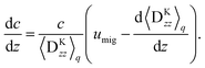 | (50) |
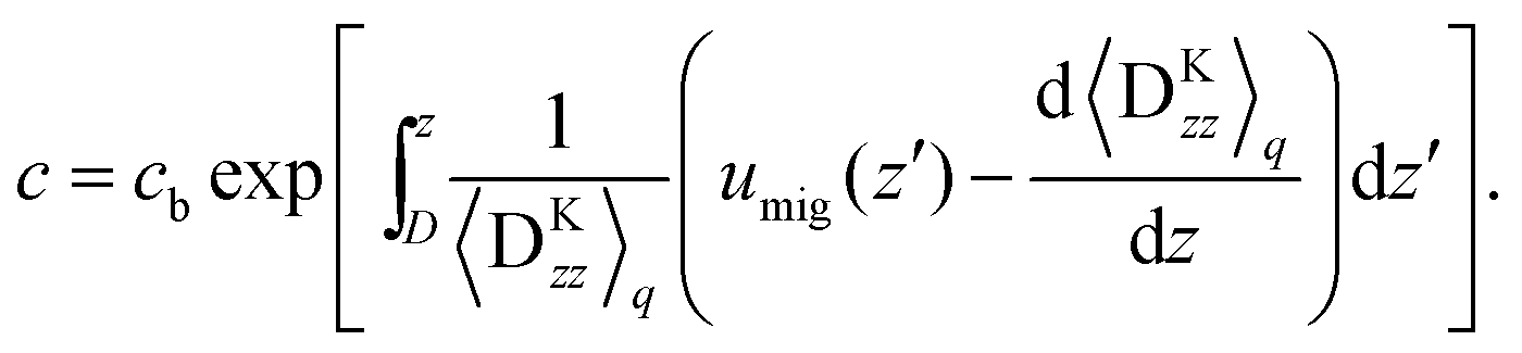
This equation shows that the migration flux and the diffusion flux are balanced at the peak of the concentration profiles. Finally the concentration profile is calculated as| | 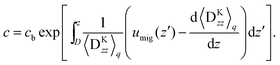 | (51) |
The resultant flow profile can be calculated as| |  | (52) |
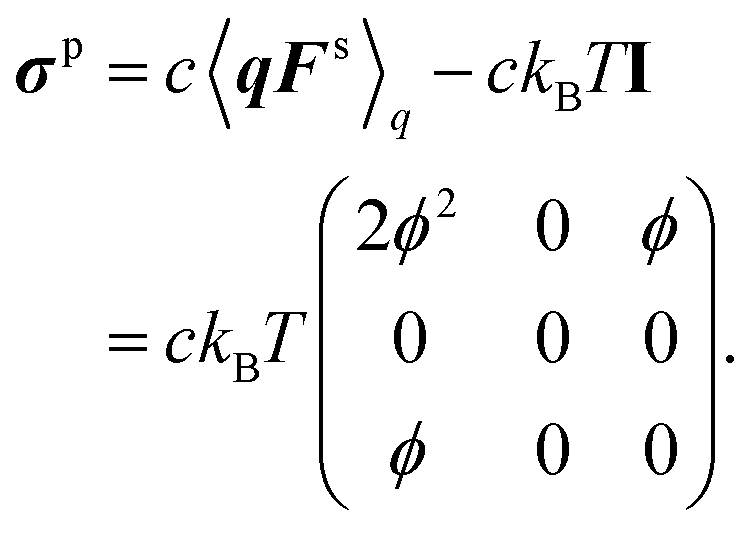
where σp is the polymeric part of the stress tensor:| | | σp = c〈qFs〉q − ckBTI. | (53) |
To obtain explicit expressions for c and δu, it is necessary to estimate umig, 〈DKzz〉q, and σp. For this purpose, eqn (43) should be analysed. However, eqn (43) is highly complicated. Even without the wall effects, it cannot be solved exactly, so several approximation methods have been proposed.44 For simplicity, all the hydrodynamic interactions are ignored; thus, the continuity equation is given as
| |  | (54) |
For the Hookian dumbbell,
eqn (54) can be solved for the second moment of
q, and for the FENE dumbbell, a pre-averaged approximation
41,42 is employed. The curved lines in
Fig. 5 are calculated using these approximations, and they exhibit good quantitative agreement with the simulation results. Appendix B gives approximate expressions for these quantities of the Hookian and FENE dumbbells.
Fig. 6(a), (c), and (e) show the concentration profiles for the applied field E = 1000E0. The points are obtained by the Brownian dynamics simulation and the curved lines are obtained by the kinetic theory. The theoretical calculations quantitatively cover the simulations well. Moreover, they reproduce the differences in the concentration near the surface between the Hookian and FENE dumbbells, as the migration velocity can be approximately proportional to 〈χ〉q (see Appendix B), and it is greatly suppressed in the Hookian dumbbells. Fig. 6(b), (d), and (f) show the nonlinear electro-osmotic mobilities with respect to the applied field. The theoretical curved lines also exhibit acceptable agreement with the simulation results. However, they are not as consistent with the simulation results under weak applied electric fields, as the equilibrium depletion layer is not considered in the kinetic theory.
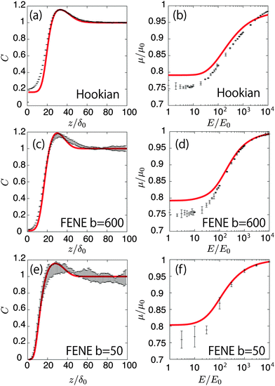 |
| | Fig. 6 (a) Concentration profiles of the Hookian dumbbell as a function of the distance from the surface. Points show the simulation results; the curved line is calculated by the kinetic theory. (b) Nonlinear electro-osmotic mobilities of the Hookian dumbbell as a function of an applied electric field. (c) and (d) same as (a) and (b), respectively, but for the FENE dumbbell with b = 600. (e) and (f) Same as (a) and (b), respectively, but for the FENE dumbbell with b = 50. | |
6 Summary and remarks
Brownian dynamics simulations are used to study nonlinear electro-osmotic behaviour of dilute polymer solutions. The simulation results agree with a toy model and analytical calculations using a kinetic theory. The main results are summarised below.
(i) Under an external plug flow, the polymer migrates toward the bulk. The concentration profile of the polymer shows a depletion layer and a single peak. The thickness of the depletion layer depends on the electric field. At the peak, the migration flux is balanced by the diffusion flux.
(ii) The growth of the depletion layer leads to an increase and saturation of the electro-osmotic mobility. This behaviour does not depend qualitatively on the rheological properties of the dumbbells.
(iii) The results of analytical calculation of the concentration and the nonlinear mobility using the kinetic theory agree with the results of the Brownian dynamics simulation. The threshold of the electric field for nonlinear growth and saturation of the mobility is much larger than that predicted by the toy model, as the diffusive flux suppresses the migration toward the bulk due to the inhomogeneous shear flow.
We conclude this study with the following remarks.
(1) Nonlinear electro-osmosis with λ ≪ δ0 has already been observed experimentally.26,27 These studies reported that the mobility increased with increasing electric field. However, nonlinear electro-osmosis with λ ≫ δ0 has not been reported experimentally; therefore, experimental verification of our findings is highly desired.
(2) It remains a future problem to determine whether the hydrodynamic interaction between the polymers and the surface plays an important role in the electro-osmosis of polymer solutions with λ ≪ δ0. In this case, the elongation of the polymers is strongly inhomogeneous under plug flow with a short Debye length; thus, more realistic chain models should be considered.
(3) Addition of charged polymers to solutions can change the direction of the linear electro-osmotic flow.7,23 When a sufficiently strong electric field is applied to this system, the flow might recover its original direction. This needs to be investigated theoretically and experimentally.
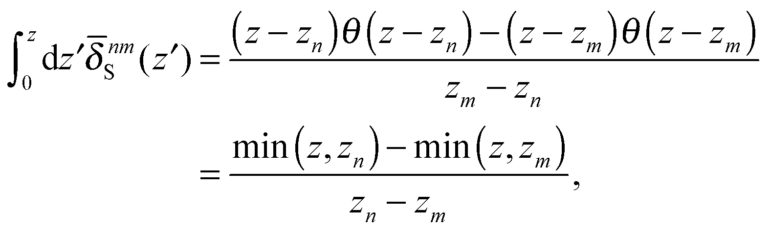
A Derivation of the velocity equation for Brownian dynamics simulation
In this appendix, the derivation of eqn (25) is explained. The velocity field induced by the polymer is given by| |  | (55) |
and the polymeric part of the stress tensor is obtained by averaging the microscopic expressions in the lateral directions as| | 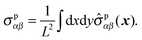 | (56) |
Here the microscopic expression of the stress tensor is given by| |  | (57) |
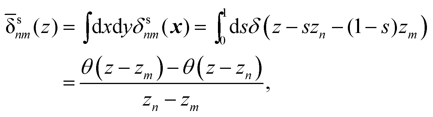
where Fnm is the force exerted on the n-th bead by the m-th bead, and δsnm(x) is the symmetrised delta function given by| |  | (58) |
The symmetrised delta function is integrated in the lateral directions as| |  | (59) |
where θ(zn − z) = 1 − θ(z − zn). Then we obtain| |  | (60) |
where min(z,zn) = zθ(z) − (z − zn)θ(z − zn). Finally, the velocity increment is expressed as| |  | (61) |
B Approximated expressions for kinetic theory
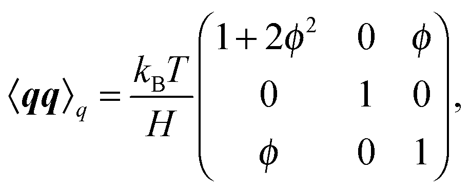
B.1 Hookian dumbbell
Eqn (54) can be rewritten in a closed form for the second moment of the spring coordinates in a steady state with an imposed plug flow. The solution is given by42| | 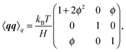 | (62) |
where| | 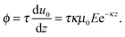 | (63) |
Therefore, we haveand the polymeric stress tensor is| | 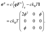 | (65) |
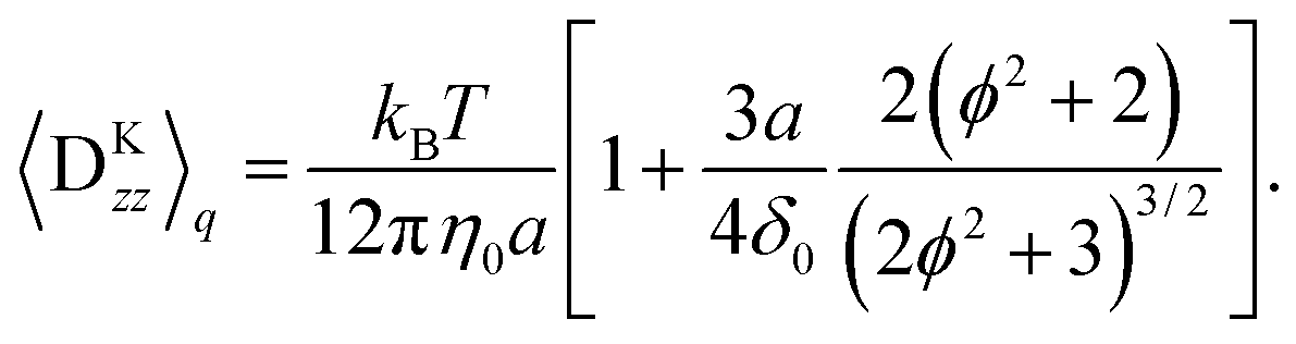
The Kirkwood diffusion constant can be estimated as| | 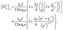 | (66) |
where the second term is split into second-order moments; thus, we obtain| | 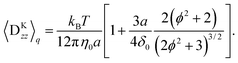 | (67) |
It is differentiated by z as| | 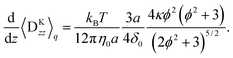 | (68) |
The migration velocity can be estimated using the splitting approximation of the averages as| | 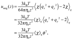 | (69) |
where| | 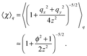 | (70) |
B.2 FENE dumbbell
The second moment of the spring coordinate for a FENE dumbbell can be obtained by pre-averaged closures of a p-FENE model.41,42 It is given by| | 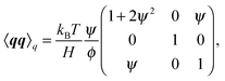 | (71) |
and| | 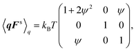 | (72) |
where| | 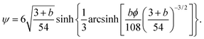 | (73) |
The polymer stress tensor is| | 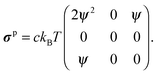 | (74) |
The Kirkwood diffusion constant is| |  | (75) |
and its derivative is| | 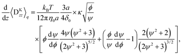 | (76) |
where| | 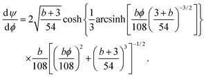 | (77) |
Finally the migration velocity is obtained as| | 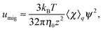 | (78) |
where| | 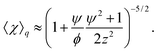 | (79) |
Acknowledgements
The author is grateful to O. A. Hickey, T. Sugimoto, R. R. Netz, and M. Radtke for helpful discussions. The author also thanks M. Itami, M. R. Mozaffari, and T. Araki for their critical reading of the manuscript. This work was supported by the JSPS Core-to-Core Program “Nonequilibrium dynamics of soft matter and information”, a Grant-in-Aid for JSPS Fellows, and KAKENHI Grant No. 25000002.
References
-
S. S. Dukhin and B. V. Derjaguin, in Surafce and Colloid Science, ed. E. Matijrvic, Wiley, New York, 1974, vol. 7 Search PubMed.
-
W. B. Russel, D. A. Saville and W. R. Schowalter, Colloidal Dispersions, Cambridge University Press, Cambridge, 1989 Search PubMed.
- T. M. Squires and S. R. Quake, Rev. Mod. Phys., 2005, 77, 977 CrossRef CAS.
- X. Wang, C. Cheng, S. Wang and S. Liu, Microfluid. Nanofluid., 2009, 6, 145 CrossRef CAS PubMed.
- F. H. J. van der Heyden, D. J. Bonthuis, D. Stein, C. Meyer and C. Dekker, Nano Lett., 2006, 6, 2232 CrossRef CAS PubMed.
- Y. W. Kim and R. R. Netz, J. Chem. Phys., 2006, 124, 114709 CrossRef PubMed.
- Y. Uematsu and T. Araki, J. Chem. Phys., 2013, 139, 094901 CrossRef PubMed.
- D. J. Bonthuis and R. R. Netz, Langmuir, 2012, 28, 16049 CrossRef CAS PubMed.
- C. Zhao and C. Yang, Electrophoresis, 2010, 31, 973 CrossRef CAS PubMed.
- C. Zhao and C. Yang, Biomicrofluidics, 2010, 5, 014110 CrossRef PubMed.
- C. Zhao and C. Yang, J. Non-Newtonian Fluid Mech., 2011, 166, 1076 CrossRef CAS PubMed.
- C. Zhao and C. Yang, Adv. Colloid Interface Sci., 2013, 201–202, 94 CrossRef CAS PubMed.
- J. Znaleziona, J. Peter, R. Knob, V. Maier and J. Ševčík, Chromatographia, 2008, 67, 5 Search PubMed.
- H. Ohshima, J. Colloid Interface Sci., 1994, 163, 474 CrossRef CAS.
- H. Ohshima, Adv. Colloid Interface Sci., 1995, 62, 189 CrossRef CAS.
- J. L. Harden, D. Long and A. Ajdari, Langmuir, 2001, 17, 705 CrossRef CAS.
- O. A. Hickey, C. Holm, J. L. Harden and G. W. Slater, Macromolecules, 2011, 44, 4495 CrossRef.
- S. Raafatnia, O. A. Hickey and C. Holm, Phys. Rev. Lett., 2014, 113, 238301 CrossRef CAS.
- S. Raafatnia, O. A. Hickey and C. Holm, Macromolecules, 2015, 48, 775 CrossRef CAS.
- O. A. Hickey, J. L. Harden and G. W. Slater, Phys. Rev. Lett., 2009, 102, 108304 CrossRef.
- X. Liu, D. Erickson, D. Li and U. J. Krull, Anal. Chim. Acta, 2004, 507, 55 CrossRef CAS PubMed.
- G. Danger, M. Ramonda and H. Cottet, Electrophoresis, 2007, 28, 925 CrossRef CAS PubMed.
- L. Feng, Y. Adachi and A. Kobayashi, Colloids Surf., A, 2014, 440, 155 CrossRef CAS PubMed.
- U. M. B. Marconi, M. Monteferrante and S. Melchionna, Phys. Chem. Chem. Phys., 2014, 16, 25473 RSC.
- F.-M. Chang and H.-K. Tsao, Appl. Phys. Lett., 2007, 90, 194105 CrossRef PubMed.
- C. L. A. Berli and M. L. Olivares, J. Colloid Interface Sci., 2008, 320, 582 CrossRef CAS PubMed.
- M. L. Olivares, L. Vera-Candioti and C. L. A. Berli, Electrophoresis, 2009, 30, 921 CrossRef CAS PubMed.
- C. L. A. Berli, Electrophoresis, 2013, 34, 622 CrossRef CAS PubMed.
- M. S. Bello, P. de Besi, R. Rezzonico, P. G. Righetti and E. Casiraghi, Electrophoresis, 1994, 15, 623 CrossRef CAS PubMed.
- R. M. Jendrejack, D. C. Schwartz, J. J. de Pablo and M. D. Graham, J. Chem. Phys., 2004, 120, 2513 CrossRef CAS PubMed.
- H. Ma and M. D. Graham, Phys. Fluids, 2005, 17, 083103 CrossRef PubMed.
- J. P. Hernández-Ortiz, H. Ma, J. J. de Pablo and M. D. Graham, Phys. Fluids, 2006, 18, 123101 CrossRef PubMed.
- D. L. Ermak and J. A. McCammon, J. Chem. Phys., 1978, 69, 1352 CrossRef CAS PubMed.
- J. R. Blake, Proc. Cambridge Philos. Soc., 1971, 70, 303 CrossRef.
- E. Wajnryb, K. A. Mizerski, P. J. Zuk and P. Szymczak, J. Fluid Mech., 2013, 731, R3 CrossRef.
- P. J. Zuk, E. Wajnryb, K. A. Mizerski and P. Szymczak, J. Fluid Mech., 2014, 741, R5 CrossRef CAS.
- J. W. Swan and J. F. Brady, Phys. Fluids, 2007, 19, 113306 CrossRef PubMed.
- Y. von Hansen, M. Hinczewski and R. R. Netz, J. Chem. Phys., 2011, 134, 235102 CrossRef PubMed.
- I. Bitsanis and G. Hadziioannou, J. Chem. Phys., 1990, 92, 3827 CrossRef CAS PubMed.
- R. L. Christiansen and R. B. Bird, J. Non-Newtonian Fluid Mech., 1977/1978, 3, 161 Search PubMed.
- R. B. Bird, P. J. Dotson and N. L. Johnson, J. Non-Newtonian Fluid Mech., 1980, 7, 213 CrossRef CAS.
-
R. B. Bird, C. F. Curtiss, R. C. Armstrong and O. Hassager, Dynamics of Polymeric Liquids, Wiley, New York, 1987, vol. 2 Search PubMed.
-
M. Doi and S. F. Edwards, The Theory of Polymer Dynamics, Oxford University Press, New York, 1986 Search PubMed.
- W. Zylka and H. C. Öttinger, J. Chem. Phys., 1989, 90, 474 CrossRef CAS PubMed.
|
| This journal is © The Royal Society of Chemistry 2015 |
Click here to see how this site uses Cookies. View our privacy policy here. 
 Open Access Article
 This Open Access Article is licensed under a
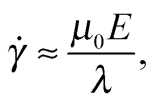
 . Here, for simplicity, we assume that the depletion length does not exceed the Debye length. The effective viscosity in the double layer is given by
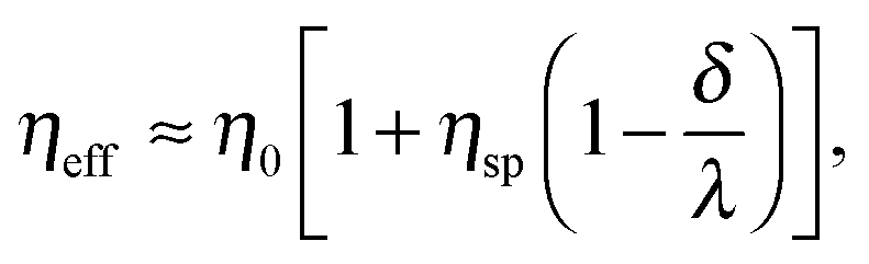


 and time scale τ = 6πη0a/4H. Different types of dumbbells are simulated using the parameters listed in Table 1.