DOI:
10.1039/C5SM01069A
(Paper)
Soft Matter, 2015,
11, 7337-7344
Conformations, hydrodynamic interactions, and instabilities of sedimenting semiflexible filaments†
Received
4th May 2015
, Accepted 7th August 2015
First published on 7th August 2015
Abstract
The conformations and dynamics of semiflexible filaments subject to a homogeneous external (gravitational) field, e.g., in a centrifuge, are studied numerically and analytically. The competition between hydrodynamic drag and bending elasticity generates new shapes and dynamical features. We show that the shape of a semiflexible filament undergoes instabilities as the external field increases. We identify two transitions that correspond to the excitation of higher bending modes. In particular, for strong fields the filament stabilizes in a non-planar shape, resulting in a sideways drift or in helical trajectories. For two interacting filaments, we find the same transitions, with the important consequence that the new non-planar shapes have an effective hydrodynamic repulsion, in contrast to the planar shapes which attract themselves even when their osculating planes are rotated with respect to each other. For the case of planar filaments, we show analytically and numerically that the relative velocity is not necessarily due to a different drag of the individual filaments, but to the hydrodynamic interactions induced by their shape asymmetry.
1. Introduction
Semiflexible filaments are fundamental constituents of micro-biological systems, where microtubules and actin filaments serve as scaffolds for cellular structures and as routes to sustain and guide cellular transport systems.1 Microtubules are also the main structural elements of cilia and sperm flagella, where their relative displacement and deformation due to motor proteins gives rise to the flagellar beat and hydrodynamic propulsion.2,3 Microtubules and flagella can be seen as elastic filaments interacting with their own flow field. The ability to visualize, assemble, and manipulate biological and artificial semiflexible polymers4–7 poses new fundamental questions on the dynamics of filaments when elastic and hydrodynamic forces compete.
The dragging of stiff rods through a viscous fluid has been studied in detail.8 A single rod does not reorient, but falls with its initial orientation. A more complex dynamical behavior can be expected and is indeed observed for semiflexible filaments when the curvature or stretching elasticity competes with the hydrodynamic interactions.9–11 Single dragged semiflexible filaments bend into a shallow V-shape to balance the higher drag at both ends12 and their end-to-end vector aligns perpendicularly to the external field.11 For strong drag, higher modes have been found to be excited; this generates W-shapes initially, which then relax back into horseshoe-like U-shape.12 Here, the dynamics seems to be constrained to the plane initially defined by the direction of the external field and the filament itself. However, these investigations address the problem from a deterministic point of view, and little attention has been paid to the dynamic stability of the resulting shapes. In all cases, the dragged and deformed semiflexible filament initially defines the settling plane, but the stability of the filament's planar shape has not been investigated as function of the external field or the relative position of possible neighboring filaments.
Here, we focus on the full three-dimensional shape of one, two, and three semiflexible filaments sedimenting in a homogeneous external field. We incorporate the hydrodynamics into the equations of motion for the filament shape via the Oseen tensor, valid in the limit of zero Reynolds number. As a result of our numerical and analytical analysis, we find that the deformations confined to a plane become unstable with respect to normal perturbations at a threshold value B1* of the strength B of the external field, which is smaller than the threshold B2* where initial, transient W-shapes become excited, see Fig. 1. Thus, with increasing strength of the external field, two instabilities and transitions to new sedimentation modes are predicted. The first transition is from a stable planar U-shape with little bending to a stationary horseshoe-like U-shape with out-of-plane bending. The second transition at stronger fields excites a metastable W-shape, also with out-of-plane bending, which then “relaxes” into a non-stationary asymmetric U-shape. As result, there exist two families of shapes, where the elastic forces are balanced by a conformation-dependent drag.
 |
| | Fig. 1 Snapshots from simulations of single filaments dragged by the external homogeneous field B = mgL2/κ, where L is the filament length, g the external field, and κ the bending stiffness. Left: For weak field (B < B1*) the filament bends into a V-shape (in dots), dominated by the χ2,z mode. Center: As the field strength increases, higher modes with an out-of-plane component are excited, and the filament drifts sideways. Right: For even stronger fields (B > B2*) further symmetries are spontaneously broken, and the filament rotates following a helical trajectory. Corresponding movie is shown in the ESI.† The vertical distance between the frames is reduced to enhance the visualization of the filament conformations. | |
We consider next the interaction between two filaments in an external field. Indeed, while the dynamics of an isolated filament is an indispensable knowledge needed to understand the case of n > 1 interacting filaments, many situations are characterized by elastic slender objects interacting via the generated flow field: cilia,7,13 sperm,14,15 and E. coli bundles16,17 are probably the most relevant from a biological point of view.
It is known that the sedimentation behavior of colloids can be quite complex. The interaction of sedimenting particles has been studied in considerable detail for spherical colloids.18,19 Two particles sediment together, but don't follow the direction of the external field, and move instead under an angle with respect to it. For more particles, many different dynamical behaviors can be found, in particular periodic motions where particles “dance” around each other.19
For dragged semiflexible filaments, the dynamical behavior is even more complex.10 In particular, we show that two filaments (Fig. 1) attract each other, repel each other, or spin around the field depending on the intensity of the external field.
We focus here on the stability of the sedimentation plane for different field intensities and on the origin of the relative velocity. In particular, we want to see whether the velocity difference is due to different shapes or to the broken up-down symmetry. For even more filaments, the dynamics becomes unsteady at much weaker external field strength than expected from the two-filaments case.
2. Model and methods
2.1 Discrete model
In the simulation, filaments of length L = b(N − 1) are represented by N mass points of mass m connected by harmonic bonds of length b, with the potential| |  | (1) |
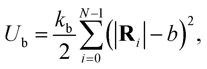
where Ri = ri+1 − ri is the vector connecting the consecutive points, i ∈ {0,…,N}, and kb is the force constant. To account for filament stiffness, we introduce the bending potential| |  | (2) |
with the bending rigidity κ.20 In addition, the mass points are exposed to an external gravitational field with the force on a particlewith the unit vector ez along the z axis of the Cartesian coordinate system (cf.Fig. 1).
Inter- and intrafilament hydrodynamic interactions substantially influence the filament dynamics. Hence, we apply the equation of motion
for the overdamped dynamics,
21 where,
ui is the background flow velocity at the position
ri of the particle,
γ0 = 3π
ηb is its friction coefficient for a fluid of viscosity
η, and
FCi is the sum of all conservative forces.
10 We compute the background flow velocity explicitly
via the Oseen tensor.
21 Thus, the final equations of motion are
| |  | (5) |
with the hydrodynamic tensor
| |  | (6) |
and
rij =
ri −
rj,
rij = |
rij|, and
![[r with combining circumflex]](https://www.rsc.org/images/entities/b_char_0072_0302.gif) ij
ij =
rij/
rij.
If needed, excluded-volume interactions are implemented via a short-range Yukawa potential between points of different filaments, which implies a minimal effective distance during the simulations. A low-amplitude white noise is added to avoid metastable states. The noise is not considered to be of thermal origin as it is chosen to be negligible compared to the other hydrodynamic and mechanical forces and barely influences the stationary settling dynamics for the considered external fields.
2.2 Parameters/methods
We set the hydrodynamic diameter of a point equal to the bond length, as in the Shish-Kabab model of ref. 10, 12 and 21, thereby fixing the aspect ratio to b/L. Lengths are measured in units of the hydrodynamic diameter b and time in units of γ0b3/κ. This choice eliminates the friction coefficient and the bending rigidity from the equations of motion. The force constant for the bonds is set to kbb3/κ = 1, resulting in a maximum extension of ±0.6% of the length over the investigated range of parameters. In these units, the external field strength mg becomes G = mgb2/κ. For convenience and an easier comparison with results of ref. 10, we characterize the external force by B = N2G, or B = mgL2/κ. For B ≪ 1, the bending rigidity dominates and the filament is essentially straight. We consider only filaments of length L = 30b in the following. For excluded volume interactions, the minimal effective distance is approximately 5b. The equations of motion are integrated with an adaptive time-stepping Velocity-Verlet algorithm.22,23
2.3 Continuum model
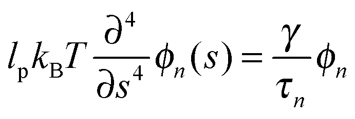
For an analytical description of the filament dynamics, we adopt a continuum model. The equation of motion of the point rν(s,t) (−L/2 ≤ s ≤ L/2) along the contour of filament ν is given by24| |  | (7) |
where fμ is the external force density and the index μ indicates the various filaments. As before, the hydrodynamic tensor H(rν(s) − rμ(s′)) comprises the Oseen tensor and the local friction. Explicitly, it reads as| |  | (8) |
Here, Θ(x) is the Heaviside function, γ = 3πη is the friction per unit length, and R = rν(s) − rμ(s′).24,25 The force density f comprises bond, bending, and gravitational forces. In the limit of a rather stiff filament, it can be written as| |  | (9) |
with the persistence length lp.26,27 In the following, we will neglect the bond term, i.e., the term with the second derivative and focus on bending stiffness only.
The expansion
| |  | (10) |
in terms of the eigenfunctions
ϕn of the biharmonic operator,
i.e.,
| |  | (11) |
with suitable boundary conditions,
26,27 leads to the equations of motion of the mode amplitudes
| |  | (12) |
The matrix representation of the hydrodynamic tensor is
| |  | (13) |
The eigenfunctions
ϕn(
s) and relaxation times
τn are well known.
5,24,27 For convenience, we summarize them in Appendix A. However,
eqn (12) is nonlinear and thus cannot straightforwardly be solved. For the current analysis, the second and forth mode are most important; they are responsible for the V- and W-shape displayed in
Fig. 1.
To characterize the numerically obtained filament conformations, we calculate the mode amplitudes
| |  | (14) |
The components of the vector
χνn indicate the importance of the mode in the Cartesian directions. For example, the mode amplitude
χν2,z measures how much the filament bends along the
z direction into a V-like shape.
As for the discrete model, we scale lengths by the filament diameter b and time by γ0b3/kBTlp. The latter is identical to the time scaling of the discrete model, since κ = kBTlp. This implies for the strength of the external force G = ρgb3/kBTlp = mgb2/κ.
3. Results
3.1 Deformation and dynamics of single filament
The filament is initially oriented along the x axis of the reference frame. After a certain time, the dragged filament reaches a stationary shape and velocity. Examples of conformational sequences for various field strengths are displayed in Fig. 1. We characterize the shapes viaeqn (14) in terms of the mode amplitudes. In Fig. 2, the most important stationary amplitudes are presented. Below a critical field B1* ≃ 1200, the filament shape is governed by planar modes (green and black lines), where χ2,z dominates and, thus, the characteristic V-shape appears.
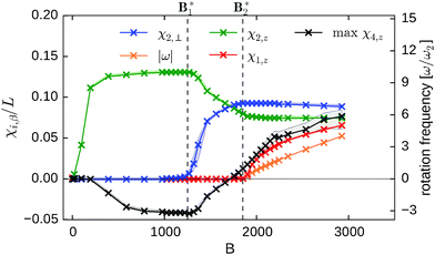 |
| | Fig. 2 Stationary mode amplitudes of a single semiflexible filament as function of the external field B. The shaded areas indicate the 66% confidence interval. When B < B1*, only planar modes are excited, and the filament stays in the plane defined by its initial orientation and the orientation of the applied field, here the xz plane. For B > B1*, an out-of-plane mode χ2,⊥ is excited. For B > B2*, the out-of-plane component χ2,⊥, the bending component χ2,z saturates, and the amplitude χ4,z becomes important (visualized in Fig. 1). In black crosses indicate the maximum value of χ4,z before it decays. The resulting shape is asymmetric and spirals around the z axis with frequency |ω|/ω2 (orange line), with ω2 the frequency of the second mode (eqn (15)). | |
In simulations restricted to a two-dimensional plane, or in three-dimensional simulations without noise,12 the filament dynamics is localized in the xz plane and filaments bend into a planar W-shape for fields B > B2* ≈ 1800. In contrast, in our three-dimensional simulations with weak noise, we find that the planer filament conformations are metastable for B1* < B < B2*, and also modes along the y axis are excited. We characterize the out-of-plane filament shape and dynamics by the mode amplitude χ2,⊥(t), where
| | | χ2,⊥(t) = χ2,x(t) + iχ2,y(t) = |χ2,⊥|eiωt. | (15) |
In the stationary state, an U-shaped and deck-chair-like conformation is assumed with out-of-plane bending (see
Fig. 1). The filament orientation is fixed and
χ2,⊥ =
χ2,y (blue line in
Fig. 2). Since its shape is asymmetric, the filament drifts sideways while settling in the external field.
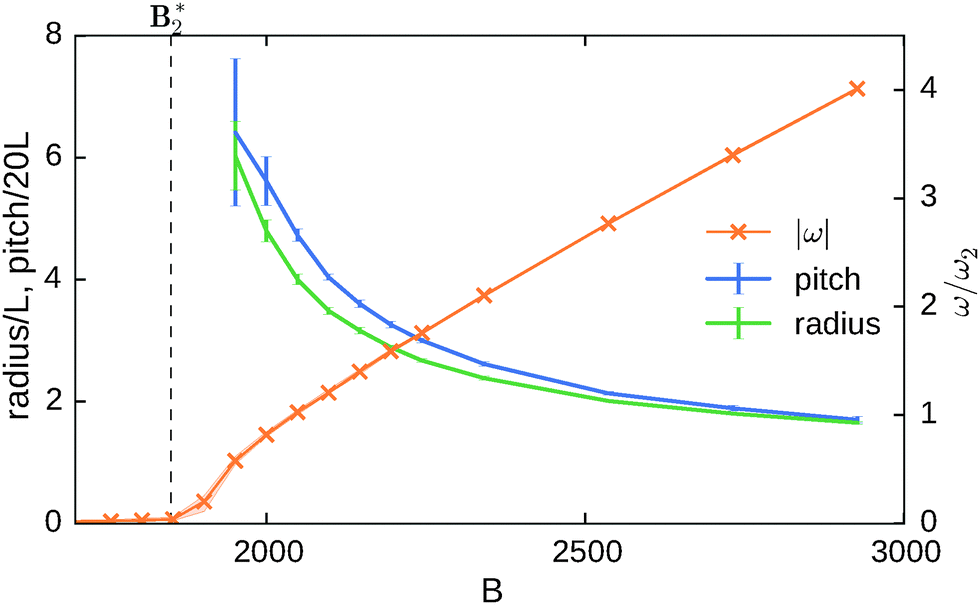
When B ≳ B2*, the mode χ4,z becomes important at early times, leading to a temporary W-shape (Fig. 1). The trajectory for B ≃ 3000, displayed in Fig. 1, shows the initial W, which later turns into an asymmetric U-shape, in which one arm is longer than the other. The appearing shape is stable; however, because of its asymmetry, the mode amplitude χ1,z is non-zero and the filament rotates around the z axis with frequency ω, see Fig. 2 (orange line), which we determined viaeqn (15). In Fig. 3, we characterize the helical trajectories by the pitch, radius, and rotation frequency (B > B2*). As the field increases the rotation frequency increases, and the helix becomes more tight because the radius decreases and the pitch shortens. The ratio between the pitch and the radius defines the helix angle α ≈ 4π/9, constant for all B > B2*. Approaching the transition point from above, the rotation frequency vanishes, and both radius and pitch diverge because the trajectory straightens.
 |
| | Fig. 3 Pitch, radius, and rotation frequency of the helical trajectories when B > B2*. The radius and pitch seem to diverge in the proximity of the transition. Bars are standard deviations. | |
In contrast, in the deterministic dynamics of previous studies,12 the W-shape was found to decay only into the stable and symmetric planar horseshoe shape.
3.2 Conformations and dynamics of two interacting filaments
3.2.1 Weak field – relative velocity.
As shown in Section 3.1, the stationary shape of a single filament in weak fields B < B1* is of V-shape, which breaks the bottom-top symmetry. This is sufficient to generate an effective attraction between sedimenting filaments with the same shape. To characterize this interaction, we compute the relative velocity Δv between the centers of mass of two filaments of equal shape along the sedimentation direction. The filaments remain localized in the xz plane and are separated by a distance d. As shown in Fig. 4, the relative velocities exhibit a significant dependence on the filament separation. We especially find that Δv ∼ d−2 for distances larger than the filament length. The distance dependence can be understood by the theoretical model introduced in Section 2.3. For the considered filament shapes,| | | r1(s,t) = (χ1,x(t)ϕ1(s), 0, χ2,zϕ2(s))T | (16) |
and r2(s,t) = r1(s,t) + dez, the general expression for the velocity difference derived in Appendix B yields| |  | (17) |
in the limit d → ∞. Evidently, the filaments attract each other due to the top-bottom asymmetry of their shapes. In the simulations, the filament shapes are determined initially by imposing the amplitude χ2,z, which is then kept fixed. The simulation results of Fig. 4 are in agreement with our theoretical prediction down to roughly the filament length. The d−2 power law is indeed a universal scaling, unaffected by the filaments shape and external field as evident from the theoretical considerations in Appendix B. The dependence of Δv on χ2,z (eqn (17)) is also verified for very small bending.
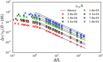 |
| | Fig. 4 Simulations of two filaments with the same imposed shape, kept constant during the simulation (B = 195). The shapes are created with the given χ2,z. The filaments lie in the same plane, parallel to the external field. The relative velocity Δv scales as d−2. The black lines correspond to the prediction of eqn (17), save for a common factor δ ≈ 11. The theory describes correctly the trend on d, and the trend on χ2,z holds up to χ2,z = 8 × 10⁻³. | |
3.2.2 Weak field – stability.
We now relax the imposed shape constraint and consider collective effects for two filaments, which are initially straight, oriented along the x axis, and displaced along the z axis by a distance d (cf.Fig. 5(a)). For easier comparison with ref. 10 and 12, we employ the dimensionless number Δ = (Aupper − Alower)/(L/2) to quantify the bending asymmetry, where Aupper,lower is the total z extension of the upper/lower filament. As indicated in Fig. 6, the filament curvature changes with time and the upper filament is bent stronger than the lower one. Fig. 6(a) and (b), show the curvature asymmetries Δ and the relative velocities for various external field strengths. Δ decreases with increasing distance d, indicating more similar shapes at larger distances. Hydrodynamic interactions lead to an attraction of the two filaments (vupper > vlower), in agreement with the imposed-shape approximation studies of the last section. Indeed, the constant-shape approximation still gives the correct (L/d)2 power-law dependence for d/L ≫ 1, while the magnitude of the deformation, χ(eff)2,z, has to be fitted. When the filaments approach each other, the generated flow field depends on the details of their shapes that, in turn, depends on the external field, hence we expect a non-universal behavior. Note that in contrast to ref. 10, we find that the upper filament bends more than the lower filament (see also Fig. 5).
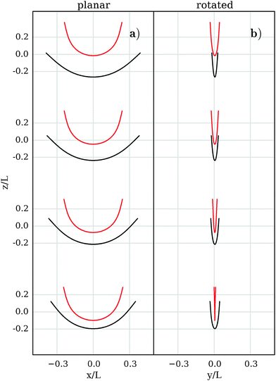 |
| | Fig. 5 Snapshots of two-filament conformations for B = 195, in time intervals Δt. (a) Co-planar sedimentation. Note that the upper filament is more bent than the lower filament, and dmin/L = 0.13. Axes to scale, z position translated. (b) The two filaments approach each other after initialization in a rotated configuration. Both filaments spin around the z axis, with the upper filament spinning faster (see Fig. 6(c and d)). | |
 |
| | Fig. 6 (a and b) Bending asymmetry Δ and relative velocity Δv of two filaments as function of the filaments distance for L/b = 30. The two filaments are in the same plane, parallel to the external field and parallel to each other. Each color corresponds to a different external field B, as indicated. The velocity v0 is the terminal velocity given by the resistive force theory for a rod. When d/L ≫ 1, the relative velocity scales as d−2. Note that filaments attract, i.e. time progresses from right to left. (c and d) Rotation angle θ and relative velocity Δv of two initially rotated filaments around the field axis by θ = 18°. The relative velocity is essentially unaffected by this change. Notably, the filaments spin toward each other decreasing the relative angle. | |
The planar configuration of a filament is also stable with respect to filament rotations around the field axis, see Fig. 5(b). Filaments that are initially displaced along the z axis (as in the previous case) and rotated with relative orientation angle θ around the external field axis spin until the relative angle vanishes, as illustrated by Fig. 6(c). Also in this case, the upper filament drifts and rotates faster than the lower one, see Fig. 6(d). The relative velocity is essentially the same as in the planar case.
Thus, two filaments sedimenting in weak fields relax toward a stable planar configuration one behind the other. The shape of the filaments is dominated by the second mode, pointing downwards, as shown in Fig. 5. This mode dominates and it breaks the mirror symmetry of the hydrodynamic interactions even for filaments of the same shape. Note that, in contrast to the single filament case, the system does not reach a stationary state velocity or shape, since the upper filament is always faster than the lower filament until the filaments touch each other.
3.2.3 Strong field.
For strong fields, we consider two filaments, which are initially displaced by 6L along the field direction. We measure the shape eigenvalues when the distance is 5L, in the quasi-stationary regime, and find that the eigenvalues exhibit the same behavior as those of a single filament. This means that for B > B1* the dynamics of each filament is dominated by the local flow field and not by the interactions with the other filament. Indeed, we find no correlations between the orientations of the out-of-plane components of the two filaments for B > B1*: the two filaments can by chance bend out-of-plane and drift in arbitrary directions.
When B > B2*, the filaments undergo the same transitions as a single filament: each of them reaches the same stationary shape and rotation velocity as an isolated filament. We find no correlations between the rotation directions of the two filaments: some filaments spin in the same direction, others in opposite directions, with no preference. This highlights the relevance of hydrodynamic interactions between two filaments for external fields weaker than B1*. At stronger fields, the non-planar configurations generate forces that compete with and dominate over hydrodynamic interactions among the filaments and the emergent behavior is, essentially, the same as that of an isolated filament.
3.3 Three filaments
Given the complex dynamics of two interacting filaments, it is interesting to consider also the collective behavior of several filaments. We find in simulations of systems with more than two filaments an intriguing collective dynamic behavior even for very weak fields (B ≃ 60) and in the absence of noise.
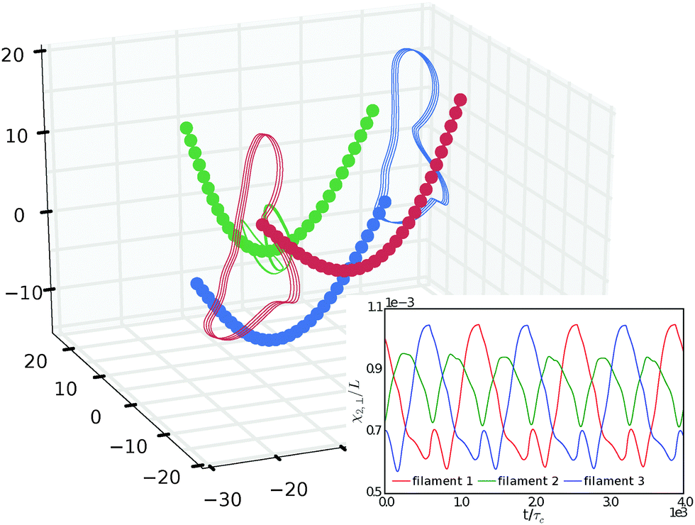
We focus here on the case of three filaments, see Fig. 7. For most (randomly chosen) initial configurations, the nearest two filaments form a bundle that settles faster than the third filament that is then left behind. However, we find also some initial configurations where all three filaments attract each other and form a bundle. In this case, the relative positions are not stationary; instead, the filaments follow a periodic trajectory, see Fig. 7 (inset). In the inset of Fig. 7, we show also that the shapes of the three filaments are not stationary. The mode amplitude χ2,z of each filament changes periodically, with a constant phase shift between them.
 |
| | Fig. 7 Three semiflexible filaments and trajectory of one bead (thick line), for the external field B ≃ 60 ≪ B1*. In this case, the filaments form a bundle, but the relative positions change periodically. Inset: Plot of χ2,z for the three filaments. Since they have the same period and constant phase shift, this is the result of a cooperative behavior. Corresponding movie is shown in the ESI.† | |
Our results for one and two filaments indicate that triggering of a time-periodic bifurcation requires strong fields. However, the three-filaments results suggest that systems with more filaments display a very complex dynamics even for weak fields due to complex hydrodynamic interactions.
4. Discussion and conclusions
We have investigated the dynamics and stability of semiflexible filaments exposed to an external homogeneous field and interacting only via hydrodynamic fluid fields. Due to the competition between hydrodynamic interactions and bending stiffness, the appearing dynamical behavior is richer than for entropy-dominated polymers or interacting rods.
We have shown that, for weak fields B < B1*, co-planar configurations of two filaments are stable upon perturbations that rotate the shapes relative to each other around the field axis. With simulations of fixed shape filaments, we have highlighted that a V- or U-shape is sufficient to break the hydrodynamic symmetry at low Reynolds numbers, leading to a relative velocity that scales with distance as (L/d)2. Hence, the difference in drag coefficients between filaments is not necessary to explain the faster settling velocity of the upper filament.
For external field strengths exceeding the critical value B1*, the hydrodynamic interactions bend the filament out of its principal plane. Simulations of a single bent filament show that the hydrodynamic forces balance the elastic force, stabilizing the out-of-plane shape. The resulting trajectory shows a drift in the direction of out-of-plane bending, superimposed to the settling motion. This is a novel result, not to be confused with the previously reported metastable W-state12 that is excited when B > B2*. A careful analysis of the eigenmodes indicates that the decay of the metastable state does not, in general, lead to the reported planar horseshoe shape, but also excites an average rotation mode with respect to the field axis (χ1,z) and our out-of-plane bending mode χ2,⊥. The filaments spin then around the field axis.
Finally, we have demonstrated that three filaments display an unexpected periodic dynamics even at field strengths far weaker than B1*. This is in contrast to the dynamics of a pair of filaments that either displays a monotonic dynamics that relaxes the attractive force (when B is weak) or a dynamics dominated by the single-filament (when B > B1*).
The interesting external fields B are in the range 101 ≲ B ≲ 104. We can estimate these parameters for biopolymers like actin or microtubules. Actin has a persistence length of lp ≃ 17 μm, an average length L ≃ 20 μm, and the bending rigidity κ ≃ 60 × 10−3 pN μm2.1 The external gravitational field, corrected for buoyancy, is about G ≈ 10−7 pN μm−1, which implies Bgravity ≃ 10−2. Microtubules, on the other hand, are stiffer, longer, and heavier with lp ∼ 1 mm, L ∼ 100 μm ≪ lp and G ≈ 10−6 pN μm−1.28 This yields the effective field strength Bgravity ≃ 10−1. An experimental test of our predictions is therefore within reach of modern centrifuges with accelerations of about 103g.
A Eigenfunctions of a semiflexible filament
The eigenvalue eqn (11) with the boundary conditions| |  | (18) |
yields the eigenfunctions| | 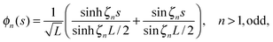 | (19) |
| |  | (20) |
The wave numbers are approximately given by ζn = (2n− 1)π/2L (n > 1), and the corresponding relaxation times by| |  | (21) |
More precise eigenfunctions are provided in ref. 24 and 27. The set of functions is complemented by the eigenfunction of the center-of-mass translation27| |  | (22) |
and that of rotation of the rodlike object| |  | (23) |
with the relaxation time| |  | (24) |
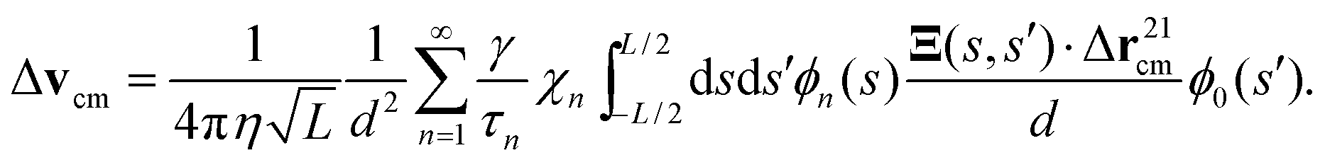
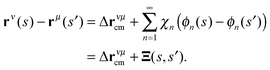
B Relative velocity of two filaments
We derive here an equation for the relative velocity between the centers of mass of two filaments. We restrict our analysis to the case of small bending amplitudes, that is equivalent to consider small external fields, and filaments of identical shape.
Since  for the exact eigenfunctions, the difference in the center-of-mass velocity Δvcm = vcm1 − vcm2 of two isolated filaments is given by
| |  | (25) |
Substitution of
eqn (12) yields
The first two terms on the right-hand side account for self-interactions of the individual filaments, the other two terms for the hydrodynamic interactions between the filaments.
We simplify our considerations by assuming identical shapes of the filaments, i.e., we set χn1 = χn2: = χn. Moreover, for the constant external force the relation applies fνnG = fν0Gδ0n independent of the particular filament. Hence, its contribution vanishes, which yields
| |  | (26) |
We are primarily interested in the distance dependence of the relative center-of-mass velocity. Hence, we additionally neglect the dyadic term in the hydrodynamic tensor (8). Moreover, the local friction term vanishes in
eqn (26), and the hydrodynamic tensor can be written as
| |  | (27) |
Using the eigenfunction expansion
eqn (10), we obtain
| |  | (28) |
With this definition, we obtain for Δ
H120n =
H210n −
H120n| |  | (29) |
In the limit
d = |Δ
r21cm| ≫ |
Ξ(
s,
s′
)|, Taylor expansion yields
| |  | (30) |
and hence,
| |  | (31) |
Substituting
x =
s/
L and setting
γ = 3π
η24 yields
| |  | (32) |
Thus, the relative velocity decreases quadratically with the distance between the filaments. There is evidently no velocity difference when Δ
r21cm is perpendicular to
Ξ(
s,
s′). In particular, there is no force between two specifically aligned rods as long as their director
χ1 is perpendicular to Δ
r21cm.
References
-
J. Howard, Mechanics of motor proteins and the cytoskeleton, Sinauer Associates, Sunderland, 2001 Search PubMed.
- S. Camalet, F. Jülicher and J. Prost, Phys. Rev. Lett., 1999, 82, 1590–1593 CrossRef CAS.
- S. Camalet and F. Jülicher, New J. Phys., 2000, 2, 24 CrossRef.
- P. E. Arratia, C. C. Thomas, J. Diorio and J. P. Gollub, Phys. Rev. Lett., 2006, 96, 144502 CrossRef CAS.
- C. H. Wiggins, D. Riveline, A. Ott and R. E. Goldstein, Biophys. J., 1998, 74, 1043–1060 CrossRef CAS.
- C. M. Schroeder, H. P. Babcock, E. S. G. Shaqfeh and S. Chu, Science, 2003, 301, 1515–1519 CrossRef CAS PubMed.
- N. Coq, A. Bricard, F.-D. Delapierre, L. Malaquin, O. du Roure, M. Fermigier and D. Bartolo, Phys. Rev. Lett., 2011, 107, 014501 CrossRef.
-
J. Happel and H. Brenner, Low Reynolds number hydrodynamics: with special applications to particulate media, Springer, 1983 Search PubMed.
- M. Manghi, X. Schlagberger, Y.-W. Kim and R. R. Netz, Soft Matter, 2006, 2, 653–668 RSC.
- I. Llopis, I. Pagonabarraga, M. Cosentino Lagomarsino and C. P. Lowe, Phys. Rev. E: Stat., Nonlinear, Soft Matter Phys., 2007, 76, 061901 CrossRef CAS.
- X. Schlagberger and R. R. Netz, Europhys. Lett., 2005, 70, 129 CrossRef CAS.
- M. Cosentino Lagomarsino, I. Pagonabarraga and C. Lowe, Phys. Rev. Lett., 2005, 94, 148104 CrossRef CAS.
- J. Elgeti and G. Gompper, Proc. Natl. Acad. Sci. U. S. A., 2013, 110, 4470–4475 CrossRef CAS PubMed.
- I. H. Riedel, K. Kruse and J. Howard, Science, 2005, 309, 300–303 CrossRef CAS PubMed.
- H. S. Fisher and H. E. Hoekstra, Nature, 2010, 463, 801–803 CrossRef CAS PubMed.
- H. C. Berg and D. A. Brown, Nature, 1972, 239, 500–504 CrossRef CAS PubMed.
- S. Y. Reigh, R. G. Winkler and G. Gompper, Soft Matter, 2012, 8, 4363 RSC.
- M. L. Ekiel-Jeżewska, T. Gubiec and P. Szymczak, Phys. Fluids, 2008, 20, 063102 Search PubMed.
- M. L. Ekiel-Jeżewska, Phys. Rev. E: Stat., Nonlinear, Soft Matter Phys., 2014, 90, 043007 CrossRef.
- J. S. Myung, F. Taslimi, R. G. Winkler and G. Gompper, Macromolecules, 2014, 4118 CrossRef CAS.
-
M. Doi and S. F. Edwards, The Theory of Polymer Dynamics, Clarendon Press, Oxford, 1986 Search PubMed.
- P. Eastman, M. S. Friedrichs, J. D. Chodera, R. J. Radmer, C. M. Bruns, J. P. Ku, K. A. Beauchamp, T. J. Lane, L.-P. Wang, D. Shukla, T. Tye, M. Houston, T. Stich, C. Klein, M. R. Shirts and V. S. Pande, J. Chem. Theory Comput., 2013, 9, 461–469 CrossRef CAS PubMed.
-
M. Galassi, et al., GNU Scientific Library Reference Manual, GNU Foundation, 3rd edn, 2013 Search PubMed.
- L. Harnau, R. G. Winkler and P. Reineker, J. Chem. Phys., 1996, 104, 6355–6368 CrossRef CAS PubMed.
- R. G. Winkler, P. Reineker and L. Harnau, J. Chem. Phys., 1994, 101, 8119–8129 CrossRef CAS PubMed.
- S. R. Aragón and R. Pecora, Macromolecules, 1985, 18, 1868 CrossRef.
- R. G. Winkler, J. Chem. Phys., 2007, 127, 054904 CrossRef PubMed.
- C. Broedersz and F. Mackintosh, Rev. Mod. Phys., 2014, 86, 995–1036 CrossRef CAS.
Footnote |
| † Electronic supplementary information (ESI) available: Two simulation animations of the sedimentation instability of isolated and non-isolated filaments. See DOI: 10.1039/c5sm01069a |
|
| This journal is © The Royal Society of Chemistry 2015 |
Click here to see how this site uses Cookies. View our privacy policy here. 
 Open Access Article
 This Open Access Article is licensed under a
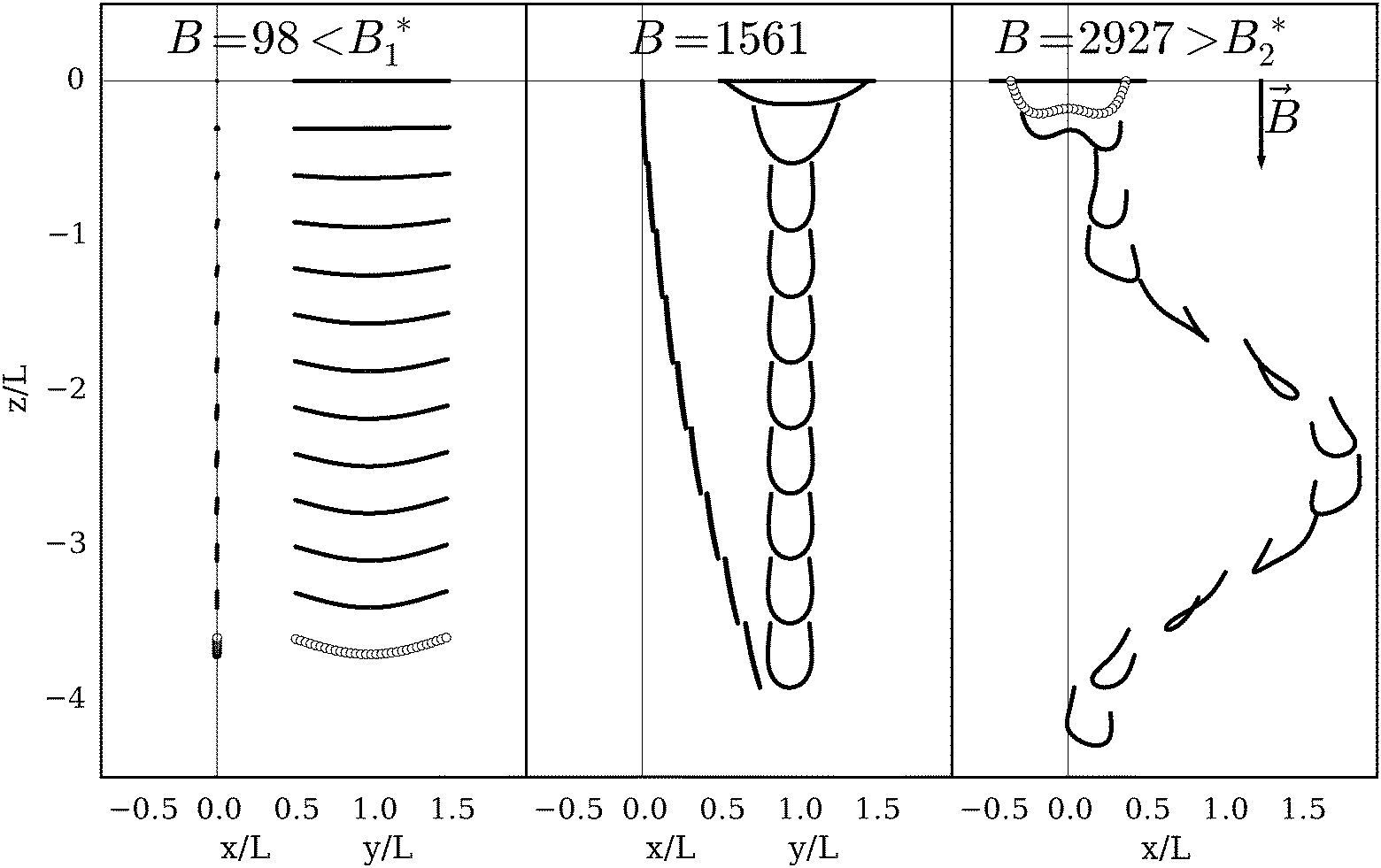


 for the exact eigenfunctions, the difference in the center-of-mass velocity Δvcm = vcm1 − vcm2 of two isolated filaments is given by