Temperature effects on a motion transmission device made from carbon nanotubes: a molecular dynamics study

Abstract

A motion transmission system made from coaxial carbon nanotubes (CNTs) is introduced. In the system, the motor is built from a single-walled carbon nanotube (SWCNT) and the converter is made from triple-walled carbon nanotubes (TWCNTs). The outer shell acts as a stator with two fixed tube ends. The inner tube (rotor 1) and the middle tube (rotor 2) can move freely in the stator. When the axial gaps between the motor and the TWCNTs are small enough and the motor has a relatively high rotational speed, the two rotors have either stable rotation or oscillation, which can be considered as output signals. To investigate the effects of such factors as the length of rotor 2, the rotational speed of the motor, and the environmental temperature on the dynamic response of the two rotors, numerical simulations using molecular dynamics (MD) are presented on a device model having a (5, 5) motor and a (5, 5)/(10, 10)/(1, 15) converter. Numerical results show that the two inner tubes can act as both rotor(s) and oscillator, simultaneously if the middle tube is longer than the inner tube. In particular, we find a new phenomenon, mode conversion of the rotation of rotor 1 by changing the environmental temperature. Briefly, rotor 1 rotates synchronously with the high-speed motor at a higher temperature or with rotor 2 at a lower temperature. The effect of radii difference among the three tubes in the bearing are also discussed by replacing the middle tube (10, 10) with different zigzag tubes.

---

1. Introduction

CNTs have been shown to have an extraordinary interlayer lubricating feature and other excellent mechanical properties at the nanoscale.^1–3 Thus, numerous studies over the past decade have focused on fabricating or designing nanodevices from CNTs, such as gigahertz oscillators,^4,5 switches,⁶ strain sensors,^7–9 bearings,¹⁰ nanopumps,^11–13 curved nanotube devices,^14,15 and motors.^16–22 In the internal layers of multi-walled carbon nanotubes (MWCNTs) both rotational and translational motions may exist, features that suggest signal transmission in a nano-device. To investigate interlayer motions in MWCNTs, Fennimore et al.²³ designed a rotational system using MWCNTs. In that system, a metal plate was glued on the outer tube and driven to rotate by electricity. Investigating the characteristics of the potential barrier of a DWCNT,²⁴ Barreiro et al.²⁵ observed the relative motion of the outer tube on the long inner tube when a thermal gradient existed along the tube axis. Hamdi et al.²⁶ proposed a rotary nanomotor made from two axially aligned MWCNTs with opposing chirality. They simulated the motions of the inner tubes when the two segments of system had different charge and found that the motion could vary from pure translational motion to pure rotation according to the combination of chirality of the tubes.

As a nanomotor made from pure carbon nanotubes is difficult to fabricate using the best available techniques,²⁷ MD simulation approaches are usually adopted to present preliminary research into prototypes of such nanodevices. For example, Kang and Hwang¹⁶ built a fluidic gas driven rotary motor with rotational frequency over 200 GHz according to their simulation results. A gradientless temperature driven motor made from DWCNTs²¹ can also attain such a high rotational speed. It is expected that temperature-controlled nanodevices would have such advantages as smaller and fewer accessories, easy operation, and good stability, compared to nanodevices driven by either electricity or fluidic gas. Besides, Shan et al.²⁸ studied the electronic transport properties of a silicon nanotube-based field-effect transistor.

In the present study, the temperature effects on the dynamic response of a nanoconverter (Fig. 1) with multiple output signals²⁹ are studied. In this system, there is a nanomotor made from a SWCNT with a TWCNT as bearing. The effects of the lengths of the two inner tubes in the bearing, the input speed of the motor, and the temperature on the dynamic behavior of the nanotube system are also considered. The purpose of the present work is to explore a way to design a controllable converter with multiple output signals.

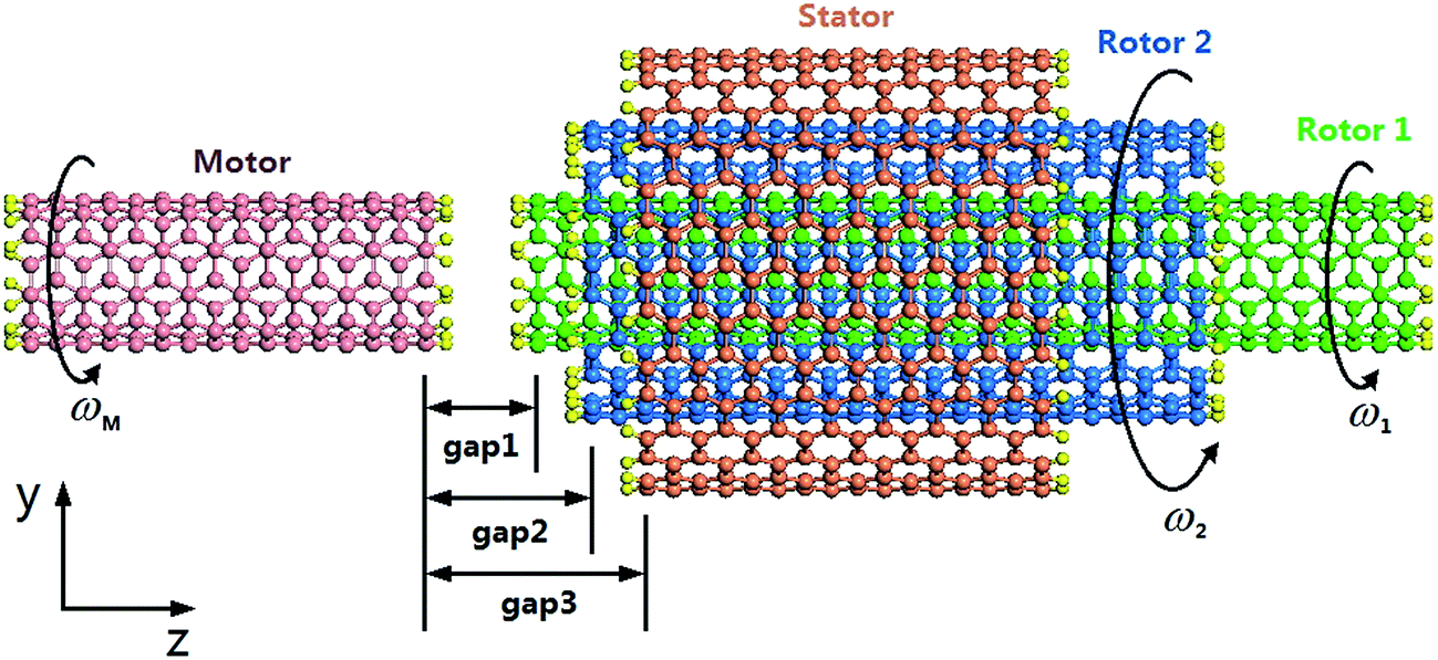Fig. 1 Model of a transmission system made from a (5, 5) SWCNT motor and a (5, 5)/(10, 10)/(15, 15) TWCNT bearing as a converter with rotor 1 ((5, 5) inner tube), rotor 2 ((10, 10) middle tube), and stator ((15, 15) outer tube), respectively. Each carbon atom at the ends of the tubes is covalently bonded with a hydrogen (small yellow) atom. ω_M, ω₁, and ω₂ are the rotational frequencies of the motor, rotor 1, and rotor 2, respectively. ω_M is a specified constant as an input signal.

2. Models and method

In the system shown in Fig. 1, the lengths of the motor, rotor 1, and the stator are fixed. For example, L₁, the length of rotor 1, is 4.18 nm, and L_s, the length of the stator, is 1.97 nm. The length of the motor, L_m, is 1.845 nm. In the present study, the length of rotor 2, L₂, varies between 0.5L₁ and 1.5L₁, to establish the relationship between the dynamic responses of the two rotors. Here we consider eight cases: L₂ = 2.46, 2.95, 3.44, 3.95 (<L₁), 4.42 (>L₁), 4.91, 5.41 and 5.93 nm.

The initial values of gap1 and gap2 are 0.335 and 0.588 nm, respectively. The value of gap3 is 0.846 nm and remains unchanged during simulation.

3. Numerical experiments

Before simulation, 100 ps of thermal bath at canonical (NVT) ensemble is applied on the system for relaxation. After relaxation, the dynamic response of the system is simulated within 5 ns at canonical NVT ensemble. The time integral increment is 1 fs. In simulation, the AIREBO potential³⁰ is used to instigate the interaction between the carbon and carbon/hydrogen atoms in the system. To determine the effects of environmental temperature on the dynamic response, three different temperatures, 150, 300, and 500 K, are considered. The simulation is carried out using LAMMPS.³¹

3.1 Dynamic response of the two rotors at environmental temperature of 150 K with fixed gap3

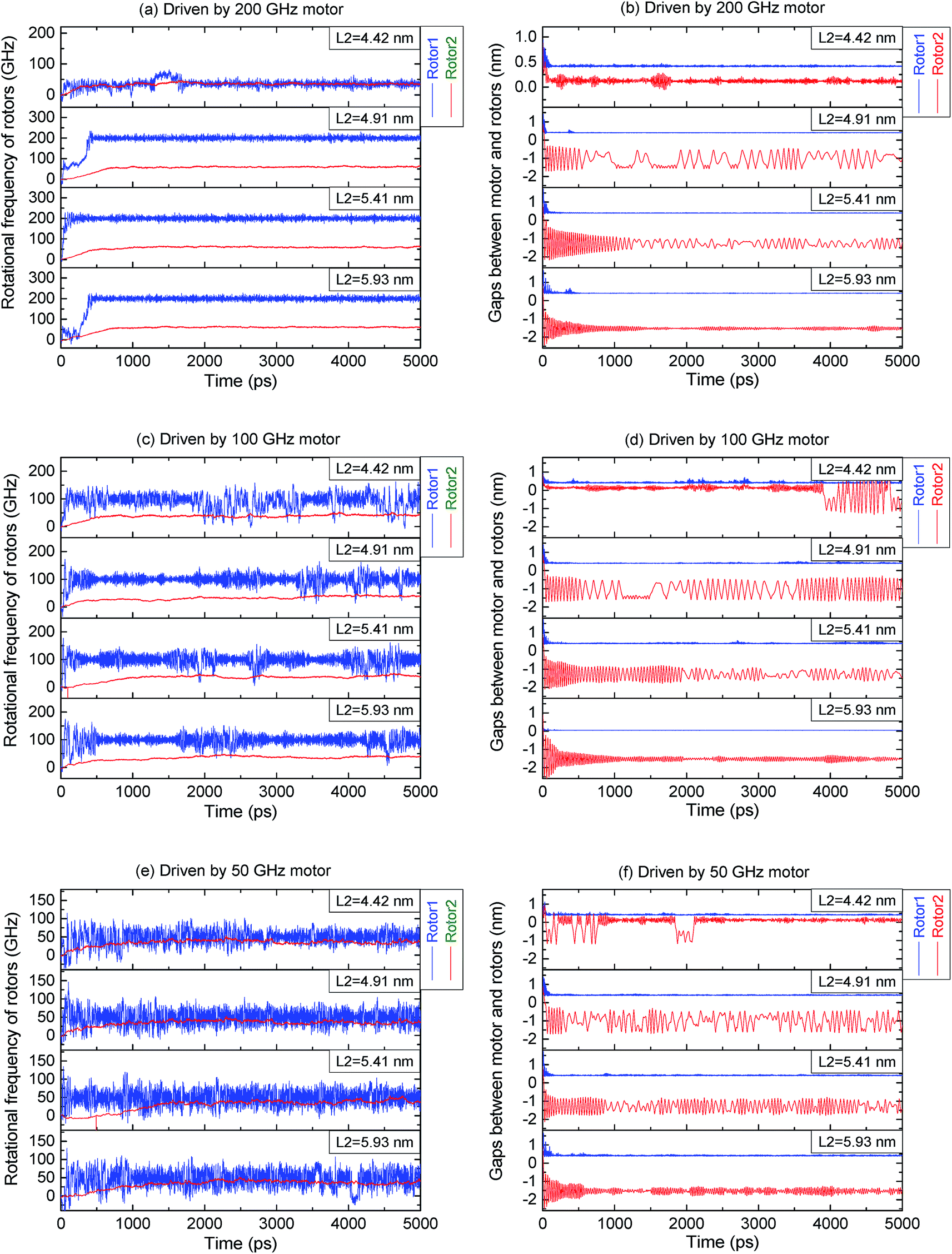
(a) When L₂ < L₁.

Fig. 2a demonstrates that rotor 1 rotates stably but more slowly than the motor. For example, ∼80 GHz of rotor 1 is far lower than the 200 GHz of the motor (ω_M = 200 GHz) (set1 in Table 1). Simultaneously, the rotational speed of rotor 2 is very small, less than 10 GHz.

Fig. 2 At canonical NVT ensemble with T = 150 K, the dynamic response of two rotors (when the length of rotor 2 is less than that of rotor 1, i.e., L₂ < L₁, and driven by the (5, 5) motor at different rotational frequencies).

Table 1 Dynamic response of rotors when driven by the (5, 5) motor with different rotational speeds at 150 K

Set1: driven by 200 GHz motor and L2 < L1 (Fig. 2a and b)
L2/nm	Rotor	Rotation of rotors	Oscillation of rotors
2.46	Rotor 1	In [0, 210] ps, ω1 increases to 81.6 GHz < 200 GHz, and rotates stably later	Gap1 varies very slightly near (VVSN) 0.430 nm
	Rotor 2	In [0, 5000] ps, ω2 is near 6.3 GHz ≪ 200 GHz	Gap2 VVSN 0.840 nm
2.95	Rotor 1	In [0, 210] ps, ω1 increases to 79.1 GHz and remains stable in [211, 1640] and [2501, 5000] ps, but a peak value of 172.9 GHz occurs in [1641, 2080] ps	Gap1 VVSN 0.431 nm except in [1880, 2290] ps with great fluctuation between 0.376 and 0.903 nm
	Rotor 2	In [0, 5000] ps, ω2 is near 9.9 GHz	Gaps2 VVSN 0.762 nm, especially in [1900, 2780] ps varying in [0.396, 1.000] nm
44	Rotor 1	In [0, 210] ps, ω1 increases to 80.5 GHz and then remains stable	Gap1 VVSN 0.429 nm
	Rotor 2	In [0, 5000] ps, ω2 is near 5.1 GHz	Gap2 VVSN 0.742 nm
3.95	Rotor 1	In [0, 1000] ps, ω1 fluctuates to 82.5 GHz and then remains stable	Gap1 VVSN 0.431 nm
	Rotor 2	In [0, 5000] ps, ω2 is near 12.2 GHz	Gap2 VVSN 0.549 nm

---

Set2: driven by 100 GHz motor and L2 < L1 (Fig. 2c and d)
L2/nm	Rotor	Rotation of rotors	Oscillation of rotors
2.46	Rotor 1	In [0, 500] ps, ω1 fluctuates to 99.6 GHz and then stays synchronous with motor (SSWM)	Gap1 VVSN 0.424 nm
	Rotor 2	In [0, 5000] ps, ω2 is near 8.1 GHz	Gap2 VVSN 0.840 nm
2.95	Rotor 1	In [0, 350] ps, ω1 increases to 99.9 GHz and then SSWM	Gap1 VVSN 0.419 nm
	Rotor 2	ω2 is between [12.4, 23.1] GHz	In [0, 3200] ps, gap2 varies between [0.954, 0.503] nm; in [3210, 5000] ps, VVSN 0.768 nm
3.44	Rotor 1	In [0, 165], ω1 increases to 99.9 GHz and then SSWM	Gap1 VVSN 0.417 nm
	Rotor 2	ω2 is between [19.7, 27.1] GHz	In [0, 5000] ps, gap2 varies between 0.931 and 0.513 nm
3.95	Rotor 1	In [0, 590] ps, ω1 increases to 99.6 GHz and then SSWM	Gap1 VVSN 0.423 nm
	Rotor 2	ω2 is between [18.5, 23.7] GHz	In [541, 5000] ps, gap2 VVSN 0.526 nm

---

Set3: driven by 50 GHz motor and L2 < L1 (Fig. 2e and f)
L2/nm	Rotor	Rotation of rotors	Oscillation of rotors
2.46	Rotor 1	ω1 fluctuates but time averagely SSWM	Gap1 VVSN 0.423 nm
	Rotor 2	In [0, 5000] ps, the average of ω2 is 2.7 GHz	Gap2 VVSN 0.840 nm
2.95	Rotor 1	ω1 fluctuates but time averagely SSWM	Gap1 VVSN 0.422 nm
	Rotor 2	In [0, 5000] ps, the average of ω2 is 3.3 GHz	Gap2 varies dramatically, but no stable oscillation
3.44	Rotor 1	ω1 fluctuates but time averagely SSWM	Gap1 VVSN 0.424 nm
	Rotor 2	In [0, 5000] ps, the average of ω2 is 3.3 GHz	Gap2 dramatically varies; in [0, 1780] and [2011, 3910] ps between 0.448 and 0.857
3.95	Rotor 1	ω1 fluctuates but time averagely SSWM	Gap1 VVSN 0.419 nm
	Rotor 2	In [0, 5000] ps, the average of ω2 is 1.5 GHz	Gap2 VVSN 0.534 nm

---

Set4: driven by 200 GHz motor and L2 > L1 (Fig. 3a and b)
L2/nm	Rotor	Rotation of rotors	Oscillation of rotors
4.42	Rotor 1	In [0, 490] ps, ω1 increases to 33.0 GHz and then remains stable	Gap1 VVSN 0.418 nm
	Rotor 2	Stays synchronous with rotor 1	Gap2 VVSN 0.118 nm
4.91	Rotor 1	In [0, 590] ps, ω1 increases to 35.8 GHz and then remains stable	Gap1 VVSN 0.413 nm
	Rotor 2	Stays synchronous with rotor 1	In [0, 780] ps, gap2 varies between [−1.746, 0.017] nm, and VVSN −1.012 nm later
5.41	Rotor 1	In [0, 410] ps, ω1 increases to 35.4 GHz and then remains stable	Gap1 VVSN 0.414 nm
	Rotor 2	Stays synchronous with rotor 1	In [0, 740] ps, gap2 varies between −2.224 and 0.069 nm
5.93	Rotor 1	In [0, 550] ps, ω1 increases to 35.5 GHz and then remains stable	Gap1 VVSN 0.417 nm
	Rotor 2	Stays synchronous with rotor 1	In [0, 620] ps, gap2 varies in [−2.624, 0.084] nm, and VVSN −1.495 nm later

---

Set5: driven by 100 GHz motor and L2 > L1 (Fig. 3c and d)
L2/nm	Rotor	Rotation of rotors	Oscillation of rotors
4.42	Rotor 1	In [0, 65] ps, ω1 increases to 100.2 GHz and SSWM	Gap1 VVSN 0.405 nm
	Rotor 2	In [0, 2100], ω2 increases to 22.6 GHz and then remains stable	In [0, 450] ps, gap2 varies in [−1.256, 0.879] nm, and varies near −0.768 nm later
4.91	Rotor 1	In [0, 100] ps, ω1 fluctuates to 100.2 GHz and SSWM	Gap1 VVSN 0.405 nm
	Rotor 2	In [0, 2750] ps, ω2 increases to 29.4 GHz and then remains stable	In [0, 2200] ps, gap2 varies harmoniously in [−1.740, 0.893] nm
5.41	Rotor 1	In [0, 410] ps, ω1 fluctuates to 100.1 GHz and SSWM	Gap1 VVSN 0.407 nm
	Rotor 2	In [0, 2650] ps, ω2 increases to 29.4 GHz and then remains stable	Gap2 shows slow damping in [−2.120, −0.076] nm
5.93	Rotor 1	In [0, 410] ps, ω1 fluctuates to 100.0 GHz and SSWM	Gap1 VVSN 0.409 nm
	Rotor 2	In [0, 2020] ps, ω2 increases to 29.0 GHz and then remains stable	In [200, 1600] ps, gap2 varies harmoniously in [−1.964, −1.081] nm

---

Set6: driven by 50 GHz motor and L2 > L1 (Fig. 3e and f)
L2/nm	Rotor	Rotation of rotors	Oscillation of rotors
4.42	Rotor 1	ω1 fluctuates but time averagely SSWM	Gap1 VVSN 0.405 nm
	Rotor 2	In [0, 1000] ps, ω2 increases to 39.2 GHz and then remains stable	Beyond [450, 5000] ps, gap2 VVSN 0.117 nm
4.91	Rotor 1	ω1 fluctuates but time averagely SSWM	Gap1 VVSN 0.405 nm
	Rotor 2	Almost no rotation in [0, 5000] ps	In [0, 1100] and [1600, 3000] ps, gap2 harmoniously varies in [−1.679, −0.359] nm
5.41	Rotor 1	ω1 fluctuates but time averagely SSWM	Gap1 VVSN 0.407 nm
	Rotor 2	In [0, 1050] ω2 increases to 33.8 GHz and then remains stable	Gap2 shows damping in [0, 5000] ps
5.93	Rotor 1	ω1 fluctuates but time averagely SSWM	Gap1 VVSN 0.409 nm
	Rotor 2	In [0, 3140] ps, ω2 increases to 39.2 GHz and then remains stable	Gap2 damps quickly in [0, 600] ps, and varies nearby −1.527 nm latter

---

From Fig. 2b we find that the minimal variation of amplitude in gap1, i.e., the oscillation of the inner tube (rotor 1, blue line), can be neglected. This phenomenon does not depend on either the length of rotor 2 (L₂ < L₁) or the rotational speed of the motor. The oscillation of rotor 2 is not stable when L₂ = 2.95 or 3.44 nm. The oscillation of rotor 2 depends very little on the rotational speed of the motor.

Fig. 2c and 3c show that rotor 1 rotates synchronously with the motor for any length of rotor 2. Hence, the attraction of the motor to rotor 1 drives their synchronous rotation when ω_M is low, e.g., <100 GHz. Synchronous rotation between the motor and rotor 1 also occurs when ω_M is 50 GHz (Fig. 2e and 3e). We conclude that synchronous rotation occurs when ω_M is lower than 100 GHz for this system.

Fig. 3 At canonical NVT ensemble with T = 150 K, the dynamic response of two rotors when L₂ > L₁, and driven by the (5, 5) motor at different rotational frequencies.

(b) When L₂ > L₁.

Fig. 3a shows an interesting result, i.e., the two rotors rotating synchronously, with their rotational speed being far lower than that of the motor. ω₁ and ω₂, the rotational frequencies of the two rotors, are ∼35 GHz (set4 in Table 1). Clearly, the attraction of the motor on rotor 1 is not strong enough to induce a high rotational speed of rotor 1. The speed is about 43% of that of rotor 1 as shown in Fig. 2a. The major reason is that the length of rotor 2 is greater than that of rotor 1, i.e., L₂ > L₁. Rotor 2 is excited to rotate at a higher speed due to the higher friction between rotor 1 and rotor 2. Although friction exists between rotor 2 and the stator, the drag of the stator on the rotation of rotor 2 is weaker than the friction between the two rotors. The value of gap2 becomes negative when L₂ > L₁ (Fig. 3b), demonstrating that the interaction between the motor and rotor 2 is also high.

Considering the two rotors as a whole component in the system, we find that the stator and the 200 GHz motor can only drive a ∼35 GHz coaxial double-rotor component. We therefore conclude that a high-speed (e.g., >200 GHz) rotary motor will drive synchronous rotors in such a system as in Fig. 1.

In Fig. 3d, as comparing with the results in Fig. 2d and f, we find that the oscillation of rotor 2 is very stable when L₂ = 4.91 nm and when rotor 2 is driven by the 100 GHz motor, i.e., both the amplitude and the period of the oscillation vary only slightly during the whole simulation except in the period of [2500, 3500] ps. The frequency of oscillation is ∼19.5 GHz during [500, 1500] ps. The amplitude is ∼0.675 nm. From Fig. 3c (L₂ = 4.91 nm) we find that rotor 1 rotates synchronously with the motor, ω₂ is ∼29 GHz, and the rotation is very stable. This observation suggests a way to design rotor 2 with a “rotation + oscillation” mode (Cai et al.⁵). This mode also exists when L₂ = 5.41 nm (Fig. 3c and d). When driven by the 50 GHz motor (Fig. 3f), the mode also exists. This observation implies that it is possible to find a stable oscillator when L₂ is within [4.91, 5.41] nm.

Comparing the rotational behavior of rotor 1 shown in Fig. 2e and 3e, we find that greater fluctuation of the rotational frequency of rotor 1 occurs when the length of rotor 2 is greater than that of rotor 1, i.e., L₂ > L₁.

3.2 Dynamic response of the two rotors at 300 K

At 300 K (higher than the 150 K mentioned above), the rotation and oscillation of the two rotors are shown in Fig. 4 and Fig. 5 when they are driven by the (5, 5) motor with different speeds. Comparison of the results in Fig. 2 and 3 at 150 K demonstrates some peculiar characteristics.

Fig. 4 At canonical NVT ensemble with T = 300 K, the dynamic response of two rotors when L₂ < L₁, and driven by the (5, 5) motor at different rotational frequencies.

Fig. 5 At canonical NVT ensemble with T = 300 K, the dynamic response of two rotors when L₂ > L₁, and driven by the (5, 5) motor at different rotational frequencies.

(a) When L₂ < L₁.

First, ω₁ and ω₂ vary between [82, 85] GHz and [10, 20] GHz respectively, when driven by the 200 GHz motor. The oscillation of the two rotors is poor, as is the case for the two rotors at 150 K.

Second, rotor 1 rotates synchronously with the motor as long as the rotational frequency of the motor is no higher than 100 GHz. Gap1 varies slightly near 0.43 nm and gap2 varies obviously for [0, 5000] ps.

Third, ω₂ is very stable when L₂ = 3.95 nm (very close to L₁), e.g., ∼22 GHz driven by the 200 GHz motor, ∼26 GHz by the 100 GHz motor and ∼27 GHz by the 50 GHz motor, when the difference between L₁ and L₂ is very small. This finding implies that ω₂ depends slightly on the rotational speed of the motor. It is significant knowledge for designing a rotor with stable rotational speed in a NEMS.

(b) When L₂ > L₁.

Fourth, the two rotors rotate synchronously only when ω_M is 200 GHz and L₂ = 4.42 nm. If L₂ > 4.42 nm, rotor 1 rotates synchronously with the motor rather than with rotor 2. At the same time, rotor 2 rotates stably with ∼60 GHz of rotational frequency, which is independent of L₂(>4.42 nm).

Fifth, when ω_M is no higher than 100 GHz, rotor 1 rotates synchronously with the motor and rotor 2 rotates very stably and the rotational speed is ∼38 GHz. In particular, ω₂ is independent of L₂(>L₁), which is significant for designing a stable nanorotor.

Sixth, the oscillation of rotor 2 performs better when driven by the 100 GHz motor with L₂ = 4.91 nm or when driven by the 50 GHz motor with L₂ = 5.41 nm.

3.3 Dynamic response of the two rotors at 500 K

(a) When L₂ < L₁.

When driven by the 200 GHz motor (Fig. 6a and b), the rotation of the rotor 1 is unstable and rotor 2 has almost no rotation or oscillation. Particularly when L₂ = 3.44 nm, the two rotors have no speed of either rotation or oscillation. Gap1 varies from 0.443 nm to 0.425 nm and gap 2 varies from 0.835 nm to 0.596 nm as L₂ changes from 2.46 nm to 3.95 nm. This effect occurs because the attraction of the motor to rotor 1 is strong and the right end of rotor 2 is between the right ends of rotor 1 and the stator. Hence, the gaps decrease with the increase of L₂.

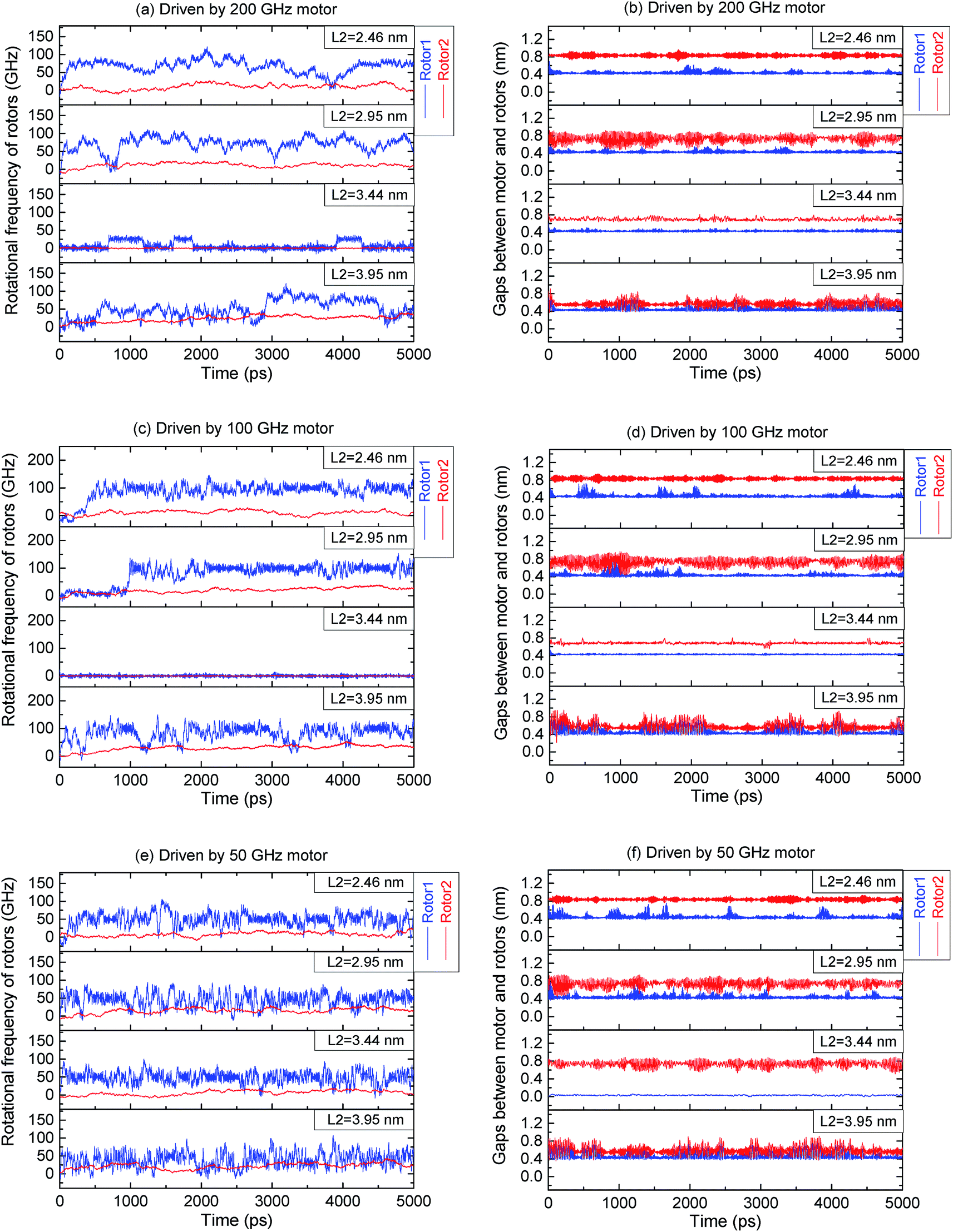Fig. 6 At canonical NVT ensemble with T = 500 K, the dynamic response of two rotors when L₂ < L₁, and driven by the (5, 5) motor at different rotational frequencies.

When driven by the 100 GHz motor (Fig. 6c and d), rotor 1 maintains synchronous rotation with the motor after a period of acceleration. Rotor 2 has a very low rotational frequency. When L₂ = 3.44 nm, the two rotors have no rotation. The oscillation of the two rotors is similar to that when they are driven by the 200 GHz motor (Fig. 6f).

When driven by the 50 GHz motor (Fig. 6e and f), rotor 1 generally rotates synchronously with the motor. When L₂ = 3.44 nm, the two rotors have no oscillation or rotation.

From the above, we find that the dynamic response of the two rotors is peculiar when L₂ = 3.44 nm. For instance, the rotors may have no rotation when the rotational speed of the motor is greater than 100 GHz or have no oscillation when the motor has a low rotational speed.

(b) When L₂ > L₁.

When driven by the 200 GHz motor (Fig. 7a and b), the dynamic response of the two rotors is very similar to that at 300 K. For instance, the two rotors rotate synchronously with a rotational speed of ∼47 GHz when L₂ = 4.42 nm. If L₂ > 4.42 nm, rotor 1 rotates synchronously with the motor, and the rotational frequency of rotor 2 is ∼67 GHz and ω₂ varies very slightly during [1000, 5000] ps.

Fig. 7 At canonical NVT ensemble with T = 500 K, the dynamic response of two rotors when L₂ > L₁, and driven by the (5, 5) motor at different rotational frequencies.

When driven by the 100 GHz motor (Fig. 7c and d), rotor 1 has no oscillation and the rotational frequency is time averagely identical to that of the motor. Rotor 2 has both perfect oscillation and very stable rotation when L₂ = 4.91 nm.

When driven by the 50 GHz motor, the two rotors rotate almost synchronously when L₂ = 4.42 nm. When L₂ > 4.42 nm, the rotation of rotor 2 is stable. Notably, the oscillation of rotor 2 is also perfect when L₂ varies within [4.91, 5.41] nm.

From the data in Fig. 2–7, we conclude that the oscillation of the rotors is very poor when L₂ < L₁ at any environmental temperature and driven by the motor with any rotational frequency. When L₂ > L₁, the value of gap2 becomes negative, which means that the joint between the motor and rotor 1 enters into the shell of rotor 2, resulting in a better dynamic response of rotor 2.

In particular, rotor 2 has very stable rotational speed and oscillation when L₂ = 4.91 nm or 5.41 nm. The major reason is that the right end of rotor 2 is locked between the right ends of the stator and rotor 1 which has no oscillation, and the interaction between the left ends of rotor 2 and the stator is strong. Therefore, we suggest a potential design of a device that has simultaneous stable oscillation and rotation from such a system with L₂ > L₁.

If L₂ = 5.93, we can obtain a pure double-rotor system with no oscillation when driven by a 200 GHz motor at any temperature. This effect occurs mainly because the total length of the motor connecting with rotor 1 is nearly equal to L₂. Hence, rotor 2 has no obvious amplitude when oscillating. On the other hand, we can also design a device in which rotor 2 acts as a pure rotator when the right (or left) end of rotor 2 is fixed within a small gap between the corresponding ends of the motor and the stator.

When L₂ is no less than 4.91 nm and the rotors are driven by a high-speed (e.g., 200 GHz) motor, the resultant effect suggests a way to convert the rotational modes of the two rotors by changing the environmental temperature. For instance, rotor 1 rotates synchronously with the motor at a lower temperature (e.g., 150 K in Fig. 3a) or with rotor 2 at a higher temperature (300 K in Fig. 5 or 500 K in Fig. 7). The reason is that the thermal vibration of atoms on tubes increases the interaction among them, and the interaction between the motor and rotor 1 is stronger than that between the two rotors.

3.4 Effects of radii difference between the two rotors

To investigate the effect of radii difference between two rotors on the dynamic response of the system, the original (10, 10) rotor 2 is replaced with zigzag tube, e.g., (16, 0) with diameter of 1.253 nm < 1.356 nm of (10, 10) tube or (19, 0) with diameter of 1.487 nm > 1.356 nm. Hence, the radii difference between (16, 0) rotor 2 and (5, 5) rotor 1 is smaller than 0.334 nm, and the radii difference between (19, 0) rotor 2 and (5, 5) rotor 1 is greater than 0.334 nm (Fig. 8).

Fig. 8 Dynamic response of two rotors driven by the 200 GHz motor and at different temperature. In the system, the length of zigzag rotor 2 is 5.112 nm. The mean value and standard deviation (SD) are counted during [4001, 5000] ps.

Due to the smaller inter tube distance between (16, 0) rotor 2 and rotor 1, the friction between two tubes is greater than that between (10, 10) rotor 2 and rotor 1. Therefore, the rotational frequency of rotor 1 is far less than motor's speed, i.e., 200 GHz. And the rotational frequency of (16, 0) rotor 2 is no less than that of (10, 10) rotor 2. The oscillation of the rotor 1 can be neglected. The oscillation of (16, 0) rotor 2 is not stable at higher temperature, e.g., 300 K or 500 K. And the value of gap2 is always positive due to the smaller radii difference between (16, 0) and (5, 5) tubes.

For the similar reason of friction between two rotors, the rotor 1 rotates synchronously with the motor and the (19, 0) rotor 2 has very small rotational frequency than the (10, 10) rotor 2. The oscillation of either rotor 1 or rotor 2 can be neglected. The value of gap2 is negative because of the higher radii difference between (19, 0) and (5, 5) than that between (10, 10) and (5, 5) tubes.

From the statistical results, one can also find that the two rotors rotate with higher speed at higher temperature. The major reason is that the interaction between two rotors increases with an increase in the temperature.

4. Conclusions

From the simulation results for the dynamic responses of the rotors in a complex transmission system, some remarkable conclusions are drawn for the design of a controllable convertor.

(1) The oscillation of the rotors is very poor when L₂ < L₁ at any environmental temperature and when they are driven by a motor with any rotational frequency.

(2) When L₂ > L₁, rotor 2 has a very stable rotational speed and oscillation when L₂ = 4.91 nm or 5.41 nm. This finding suggests the development of a nano-device with co-existence of oscillation and rotation.

(3) When L₂ is slightly greater than L₁, the two rotors rotate synchronously when driven by a high-speed motor.

(4) Rotor 2 has no oscillation if L₂ is close to the sum of L_m and L₁ or if there is a small axial gap between the right or left ends of rotor 1 (together with the motor) and the stator.

(5) When L₂ is no less than 4.91 nm and the rotors are driven by a high-speed (e.g., 200 GHz) motor, it is possible to adjust the synchronous rotation mode of rotor 1 (with either the motor at a lower temperature or with rotor 2 at a higher temperature) by changing the environmental temperature.

(6) Using different zigzag tube to act as rotor 2, the radii difference between two rotors leads to different output of the rotational frequency and oscillation of the two rotors. At different temperature, the same rotor 2 has different output rotational speed.

Acknowledgements

The authors are grateful for the financial support from the National Natural-Science-Foundation of China (Grant Nos. 50908190, 11372100).

References

1. J. Cumings and A. Zettl, Science, 2000, 289, 602–604.
2. R. Zhang, Z. Ning, Y. Zhang, Q. Zheng, Q. Chen, H. Xie, Q. Zhang, W. Qian and F. Wei, Nat. Nanotechnol., 2013, 8, 912–916.
3. Z. Qin, Q. H. Qin and X. Q. Feng, Phys. Lett. A, 2008, 372, 6661–6666.
4. Q. Zheng and Q. Jiang, Phys. Rev. Lett., 2002, 88, 045503.
5. K. Cai, H. Yin, Q. H. Qin and Y. Li, Nano Lett., 2014, 14, 2558–2562.
6. A. Subramanian, L. Dong, B. J. Nelson and A. Ferreira, Appl. Phys. Lett., 2010, 96, 073116.
7. W. Qiu, Y. Kang, Z. K. Lei, Q. H. Qin and Q. Li, Chin. Phys. Lett., 2009, 26, 080701.
8. W. Qiu, Y. L. Kang, Z. K. Lei, Q. H. Qin, Q. Li and Q. Wang, J. Raman Spectrosc., 2010, 41, 1216–1220.
9. W. Qiu, Q. Li, Z. K. Lei, Q. H. Qin, W. L. Deng and Y. L. Kang, Carbon, 2013, 53, 163–168.
10. C. Zhu, W. Guo and T. Yu, Nanotechnology, 2008, 19, 465703.
11. S. Joseph and N. Aluru, Phys. Rev. Lett., 2008, 101, 064502.
12. A. Lohrasebi and Y. Jamali, J. Mol. Graphics Modell., 2011, 29, 1025–1029.
13. J. Zhao, L. Liu, P. J. Culligan and X. Chen, Phys. Rev. E: Stat., Nonlinear, Soft Matter Phys., 2009, 80, 061206.
14. K. Cai, H. Cai, H. Yin and Q. H. Qin, RSC Adv., 2015, 5, 29908–29913.
15. K. Cai, H. Cai, J. Shi and Q. H. Qin, Appl. Phys. Lett., 2015, 106, 241907.
16. J. W. Kang and H. J. Hwang, Nanotechnology, 2004, 15, 1633–1638.
17. Z. Tu and X. Hu, Phys. Rev. B: Condens. Matter Mater. Phys., 2005, 72, 033404.
18. J. Vacek and J. Michl, Adv. Funct. Mater., 2007, 17, 730–739.
19. Z. Xu, Q.-S. Zheng and G. Chen, Phys. Rev. B: Condens. Matter Mater. Phys., 2007, 75, 195445.
20. B. Wang, L. Vuković and P. Král, Phys. Rev. Lett., 2008, 101, 186808.
21. K. Cai, Y. Li, Q. Qin and H. Yin, Nanotechnology, 2014, 25, 505701.
22. K. Cai, Y. Li, H. Yin and Q. H. Qin, Mech. Ind., 2015, 16, 110.
23. A. Fennimore, T. Yuzvinsky, W.-Q. Han, M. Fuhrer, J. Cumings and A. Zettl, Nature, 2003, 424, 408–410.
24. R. Saito, R. Matsuo, T. Kimura, G. Dresselhaus and M. Dresselhaus, Chem. Phys. Lett., 2001, 348, 187–193.
25. A. Barreiro, R. Rurali, E. R. Hernandez, J. Moser, T. Pichler, L. Forro and A. Bachtold, Science, 2008, 320, 775–778.
26. M. Hamdi, A. Subramanian, L. Dong, A. Ferreira and B. J. Nelson, IEEE ASME Trans. Mechatron., 2013, 18, 130–137.
27. T. Yuzvinsky, A. Fennimore, A. Kis and A. Zettl, Nanotechnology, 2006, 17, 434–438.
28. G. Shan, Y. Wang and W. Huang, Phys. E, 2011, 43, 1655–1658.
29. K. Kim, X. B. Xu, J. H. Guo and D. L. Fan, Nat. Commun., 2014, 5, 3632.
30. S. J. Stuart, A. B. Tutein and J. A. Harrison, J. Chem. Phys., 2000, 112, 6472–6486.
31. LAMMPS, LAMMPS Molecular Dynamics Simulator, http://lammps.sandia.gov/, 2013.

---

Footnote

† Electronic supplementary information (ESI) available. See DOI: 10.1039/c5ra10470j

---