Atomic approach to the optimized compositions of Ni–Nb–Ti glassy alloys with large glass-forming ability

Abstract

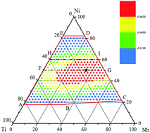
In the present study, we first constructed a long-range empirical potential for a ternary Ni–Nb–Ti system consisting of fcc, bcc and hcp metals, and then employed the verified potential in atomic simulations to study the formation of Ni–Nb–Ti glassy alloys. Atomic simulations derived a pentagon composition region of the Ni–Nb–Ti system, within which glassy alloys are inclined to form. Furthermore, the driving force for the transformation from a crystalline solid solution to a glassy alloy could be correlated to the glass-forming ability (GFA) of a particular alloy. The GFA of ternary Ni–Nb–Ti alloys with various compositions were assessed on the basis of atomic simulation results, obtaining an optimized composition region, within which the alloys possess larger GFA, as well as an optimum composition with the largest GFA. The optimum alloy is expected to be the most stable and the size of the obtainable glass may be the largest in the ternary Ni–Nb–Ti system. The optimized composition region and optimum composition could provide guidance to design the compositions of Ni–Nb–Ti metallic glasses.

---

1. Introduction

Due to their remarkable properties, such as high elastic modulus, good corrosion resistance and high strength, bulk glassy alloys (BMG) are considered to have broad prospects in industrial applications.^1–6 Among the BMG, lots of Ni-based BMG have been produced by copper mold casting, which reveals good ductility.^7–11 As representative Ni-based BMG, Ni–Nb–Ti metallic glasses exhibit high compressive fracture strength of over 3 GPa and high thermal stability.^12,13 In particular, the Ni–Nb–Ti alloys have been focused on due to their intriguing properties such as considerable shape memory effect and pseudo-elasticity and hence could be used as functional materials for micro-electromechanical system devices.^14,15 These findings stimulated us to study the formation of ternary Ni–Nb–Ti glassy alloys, which would facilitate our understanding of the underlying glass formation mechanism.

Researchers in the BMG area focus on searching for bulk metallic glass with large glass-forming ability (GFA).^16,17 To search for the desired metallic glass formers, the empirical rules, such as deep eutectic criteria,¹⁸ atomic size difference rule¹⁹ and Inoue's rules,²⁰ have been put forward, but some related issues are not solved yet.²¹ As a consequence, it is necessary and significant to develop a model capable of predicting the GFA of glassy alloys so as to design optimized glassy alloys with large GFA.^21–23 From a physical perspective, GFA can be deemed as the intrinsic property of an alloy and is predominated by the interactions of the constituent atoms. Consequently, one is able to utilize an atomic approach to derive the GFA from the potential that represents the prime atomic interaction.

To give a comprehensive consideration of the formation of ternary Ni–Nb–Ti glassy alloys, the glass formation region (GFR) is first taken into account. The GFR indicates the alloy composition region of the system within which glassy alloys could be fabricated by certain production techniques.²⁴ Once the GFR is determined, the GFA of glassy alloys with various compositions within the GFR could be evaluated through some simulation methods.^23,25

Considering the preparation process of glassy alloys, glass formation is occurred due to the suppression or failure of crystallization, or the result of a stabilized state inherited from liquids below the glass transition temperature. As the glassy alloys always undergo a nonequilibrium process, owing to the kinetic restrictions, intermetallics with complex structures are frequently suppressed from nucleating or growing, leading to the formation of either simple structured crystals or disordered phases.²⁴ It can be deduced that the major competing phase against glassy alloys is the crystalline solid solution with simple structures, i.e., body-centered cubic (bcc), face-centered cubic (fcc), or hexagonal close packed (hcp), considering the suppressing of the formation of intermetallics.²⁶ In fact, the formation enthalpy difference between amorphous and crystalline alloys is approximately considered as the driving force for amorphization of a solid solution, which can correlate to the GFA of a particular alloy.²⁵ It is deduced that the larger the driving force, the more easily a glassy alloy can form, or the lower the critical cooling rate, or the larger the critical casting size. In consequence, the GFA could be evaluated based on the magnitude of the driving force for metallic glass formation.

In the literature, atomic simulations usually focus on the formation and structure of those metallic glasses whose constituent metals have two different structures, i.e. fcc–bcc, fcc–hcp, or bcc–hcp.^25,27–29 In the present research, a long-range realistic empirical potential was built for ternary Ni–Nb–Ti metallic system with three different constituent structures (fcc, bcc, and hcp). After that, the potential was utilized in atomic simulations to study the formation of Ni–Nb–Ti glassy alloys. According to the atomic simulation results, the GFA of Ni–Nb–Ti alloys were estimated and the optimized compositions with large GFA were derived.

2. Ni–Nb–Ti interatomic potential

Recently, Dai and Li put forward a long-range empirical potential (LREP) that can be applied in transition metallic systems comprising bcc, fcc, or hcp metals.^30–32 The LREP is utilized in the present research due to its efficiency and validity in expressing the atomic interactions of transition metallic systems. Therefore, the LREP energy E_i of an atom i can be computed by the following equations:

V(r_ij) = (r_c1 − r_ij)^m(c₀ + c₁r_ij + c₂r_ij² + c₃r_ij³ + c₄r_ij⁴), 0 < r_ij ≤ r_c1 (2)

ϕ(r_ij) = α(r_c2 − r_ij)ⁿ, 0 < r_ij ≤ r_c2 (3)

m, n, α, and c_i are the LREP parameters to be determined in the fitting procedure. r_c1 and r_c2 are the cutoff distance of the LREP. The details on eqn (1)–(3) can be found in ref. 28. From eqn (1)–(3), it can be found that the LREP energy converges to zero continuously and smoothly at the cutoff distances, therefore obviating the energy leaps and force leaps as well as the related unphysical behaviors during atomic simulations. Compared with other potentials such as the MEAM potential proposed by Baskes,³³ the LREP greatly simplifies the computation of interactions without considering the angular factors, which is reasonable in transition metallic systems while the metallic bonding exhibits a non-directional feature. Applying the LREP rather than the MEAM, the time cost of an atomic simulation can be reduced to a fraction between one fifth and one tenth, indicating a much faster running speed. The LREP can also be applied in metals with different structures (fcc, bcc, and hcp), while the MEAM meets some problems when applied in bcc metals.

In the Ni–Nb–Ti system, LREP parameters for Ni–Ni, Nb–Nb, Ti–Ti, Ni–Nb, Ni–Ti, and Nb–Ti interactions are requisite. The Ni–Ni and Nb–Nb LREP parameters have been given in ref. 29 and were directly employed in the present work. Therefore, it is just required to determine the Ti–Ti LREP parameters by fitting to the reference physical properties (lattice constants, cohesive energies, and elastic modulus) of hcp-Ti experimentally. To fit Ni–Nb, Ni–Ti, and Nb–Ti cross LREP, intermetallics with different compositions and atomic configurations are utilized to make sure that the obtained LREP is good enough to express the atomic interactions in different atomic configurations. Without enough experimental data for Ni–Nb–Ti intermetallics, especially the binary Nb–Ti compounds, ab initio calculations based on density functional theory (DFT) were conducted using CASTEP.^34,35 In the ab initio calculations, nonlocal ultrasoft pseudopotentials were employed to represent the electron–ion interaction. The energy cutoff for the plane-wave basis was 700 eV and the Brillouin zones of various structures were sampled with the same k-points spacing, which approximately equals to a mesh of 20 × 20 × 20 for a bcc unit cell. The exchange–correlation functional was constructed based on the generalized gradient approximation of Perdew and Wang (PW91).³⁶ Those setting parameters were verified to make sure that the calculation satisfied the requirements for energy convergence and precision. At first, geometry optimization was conducted to acquire the lattice constants and enthalpies of the intermetallics. The elastic moduli of the optimized intermetallics were consequently computed. The cohesive energies of the intermetallics are able to be obtained from the enthalpies. The formation heats and cohesive energies can be deduced from each other. For convenience, only the cohesive energies are listed in this article. The constructed Ni–Nb–Ti LREP parameters are presented in Table 1. The physical properties (lattice constants, cohesive energies, elastic moduli, and bulk modulus) of hcp-Ti obtained from LREP and experimentally^37–39 are shown in Table 2. The physical properties of intermetallics in binary Ni–Nb, Ni–Ti, and Nb–Ti systems obtained from the LREP and experiment^28,40 (or ab initio calculations) are exhibited in Tables 3, 4, and 5. It can be seen that the physical properties obtained from LREP and experimentally (or ab initio calculations) exhibit consistency, proving the validity of the constructed LREP.

Table 1 The six sets of constructed LREP parameters for the Ni–Nb–Ti system

	Ni	Nb	Ti	Ni–Nb	Ni–Ti	Nb–Ti
m	4	4	4	4	4	4
n	5	8	4	6	5	6
rc1 (Å)	5.768881	4.802790	5.795909	5.333995	4.420312	5.241036
rc2 (Å)	7.245217	6.818734	6.957239	5.041915	7.818882	6.880792
c0 (10^−19 J)	0.452613	16.724606	0.549500	5.984657	2.450642	2.227142
c1 (10^−19 J/Å^m+1)	−0.550598	−22.895200	−0.623598	−7.564475	−2.652920	−3.162071
c2 (10^−19 J/Å^m+2)	0.249231	11.810592	0.273602	3.592397	1.159837	1.746392
c3 (10^−19 J/Å^m+3)	−0.049850	−2.696127	−0.054871	−0.752354	−0.261233	−0.434629
c4 (10^−19 J/Å^m+4)	0.003751	0.228753	0.004280	0.057993	0.029584	0.040796
α (10^−19 J/Å^n)	0.002146	0.000473	0.032226	0.125790	0.005924	0.004534

---

Table 2 Physical properties (lattice constants (a, c Å), cohesive energies (E_c, eV), bulk modulus (B₀, Mbar), elastic constants (C_ij, Mbar)) of hcp-Ti obtained from the LREP (first line) and the experimental data (second line)^33–35

hcp-Ti	a	c	Ec	C11	C12	C13	C33	C44	B0
Fitted	2.946	4.681	4.845	1.647	0.729	0.683	1.863	0.412	1.039
Exprt	2.95	4.68	4.85	1.624	0.92	0.69	1.807	0.467	1.05

---

Table 3 Physical properties of the Ni–Nb intermetallics obtained from the LREP (first line) and those from ab initio calculations (second line)^36–38

	Nb3Ni		NbNi	NbNi3
	L12	D019	B2	L12	D019
a or a, c or a, b, c (Å)	3.864	5.433, 4.661	3.165	3.721	5.213, 4.395
	4.05	5.655, 4.765	3.095	3.70	5.151, 4.342
Ec (eV)	6.546	6.597	6.110	5.443	5.427
	6.707	6.648	6.047	5.439	5.478
B0 (Mbar)	1.466	1.304	2.205	1.892	2.175
	1.765	1.513	2.166	1.898	2.123

---

Table 4 Physical properties of the Ni–Ti intermetallics obtained from the LREP (first line) and those from ab initio calculations (second line) or experiment data (indicated by asterisk)³²

	Ni3Ti		NiTi	NiTi2	NiTi3
	L12	D024	B2	E93	L12
a or a, c (Å)	3.578	5.052, 8.339	2.933	11.139	3.833
	3.618	5.101, 8.307*	3.007*	11.293*	3.936
Ec (eV)	5.182	5.175	4.932	5.079	4.839
	5.080	5.095	5.062	5.039	4.868
B0 (Mbar)	1.939	1.855	1.528	1.260	1.205
	1.941	1.882	1.618	1.418	1.281

---

Table 5 Physical properties of the Nb–Ti intermetallics obtained from the LREP (first line) and those from ab initio calculations (second line)

	Nb3Ti	NbTi	NbTi3
	L12	B2	L12
a (Å)	4.141	3.278	4.160
	4.183	3.263	4.123
Ec (eV)	6.665	6.117	5.463
	6.666	6.135	5.446
B0 (Mbar)	1.299	1.379	1.261
	1.346	1.365	1.236

---

It is significant to assess the reliability of the LREP in a non-equilibrium environment by comparing the equation of state (EOS) deduced from the LREP with the Rose Equation (RE).⁴¹ The EOS for the metals and intermetallics obtained from the LREP and the RE are displayed in ESI Fig. S1 and S2.† It can be seen that the major part of the energy curve obtained from the LREP exhibits good consistency with the RE in the overall variation range. Although deviations between the blue and red dot curves in Fig. S2† can be seen, the deviations emerge in the vicinity of a = 1.5a₀ which are so far from equilibrium that it hardly takes place in reality. Therefore, it is considered that the Ni–Nb–Ti LREP is able to describe the atomic interactions in a non-equilibrium environment reasonably.

3. Atomic simulation methods

As discussed in Section 1, the nucleation and growth of intermetallic compounds were suppressed due to kinetic restrictions, and the intermetallics were hardly observed during the short time of the simulation process (several nanoseconds). Consequently, the prime competing phase against amorphous alloys is the fcc, bcc, or hcp solid solution, especially when the alloy composition is located close to the pure metals. Therefore, one can translate the issue involved with the GFR of Ni–Nb–Ti system into that of comparing the energy stability of a crystalline solid solution with its corresponding amorphous state (glassy alloy). The solid solution model has been successfully applied in several ternary metallic systems such as Cu–Zr–Al and Ni–Zr–Al systems to investigate the formation of ternary glassy alloys.²³

Applying the Ni–Nb–Ti LREP, a sequence of molecular dynamics (MD) simulations were first performed employing Large-scale Atomic/Molecular Massively Parallel Simulator (LAMMPS) packages⁴² to investigate the GFR of Ni–Nb–Ti system. During the atomic simulations, fcc, bcc and hcp solid solutions were built considering the fact that the stable structures of Ni, Nb, and Ti metals at the simulation temperature (300 K) are fcc, bcc, and hcp, respectively. The structure of a solid solution was determined according to the major component of the alloy. The fcc solid solution comprises 2916 (9 × 9 × 9 × 4) atoms, the bcc solid solution comprises 3456 (12 × 12 × 12 × 2) atoms, and the hcp solid solution comprises 3328 (13 × 8 × 8 × 4) atoms. For both the fcc and the bcc solid solutions, the x, y, and z axes are parallel to the [100], [010], and [001] crystalline orientations, respectively. In the hcp solid solutions, the x, y, and z axes are parallel to the [112̄0], [1̄100], and [0001] crystalline orientations, respectively. Periodic boundary conditions were set in the x, y, and z axes. In constructing the solid solutions, the solvent atoms were replaced stochastically by a set number of solute atoms to acquire an expected concentration. MD simulation was performed in the framework of an isothermal–isobaric ensemble with a time step of 5 femtoseconds. The simulation proceeded at 300 K and 0 Pa for 1 million time steps (5 nanoseconds) to achieve a stable state.

In addition to the MD simulation, a sequence of Monte Carlo (MC) simulations was conducted to calculate the formation enthalpy of the solid solutions.⁴³ The initial solid solutions were constructed analog to those conducted in the MD simulation. Periodic boundary conditions were applied in the three axes. MC simulations proceeded at 300 K and 0 Pa under the isothermal–isobaric ensemble.⁴⁴ During the relaxation period of the solid solutions, the fractional coordinates of atoms in the simulation box were fixed, while the simulation box either expanded or contracted. In other words, the atoms cannot move relative to the simulation box but move along with the simulation box. In this way, the MC simulation proceeded in the box deformation mode and the solid solutions can achieve the minimum energy state by adjusting the lattice constants while the crystallographic symmetry remained invariable. The relaxation period for solid solutions towards the minimum energy state lasted for thousands of steps. The stable solid solutions preserved the initial structure with lattice constant, which was usually different from the initial settings.

To investigate the structural variation in detail, the pair correlation functions⁴⁵ and atomic projections were employed to analyze the atomic coordinates based on the atomic simulations. The total pair correlation functions g(r) and the partial pair correlation functions of atoms A and B g_AB(r) can be computed by:

and

Details for eqn (4) and (5) can be found in ref. 45. The g(r) presents the average radial arrangements of neighboring atoms around a particular atom, which can reflect the long-range order of the atomic configurations. For ordered structures such as crystalline solids, the g(r) shows a sequence of peaks, while for disordered structures such as liquids or amorphous solids, the g(r) reveals a sequence of oscillating peaks, which decays and approaches one at long distance. In consequence, the g(r) can be used to characterize the crystalline or amorphous atomic configurations of the simulated alloys.

In addition to the pair correlation functions, Voronoi tessellation⁴⁶ was adopted to inspect the structure variation of the simulated atoms. The tiny facets of Voronoi polyhedra (area lower than 1% of the average area) were excluded in the statics of the coordination number and the Voronoi index. Based on Voronoi tessellation, the coordination number and Voronoi polyhedra can be analyzed, which uncovers the information of the neighboring atoms within a given cutoff radius. The variation of atomic arrangements contributes to the distinction between crystalline and amorphous atomic configurations, which assists us in characterizing the atomic structure variation.

4. Metallic glass formation in the Ni–Nb–Ti system

To verify the reliability of the simulated glass formation revealed by the MD simulations, the atomic configurations of the simulated metallic glasses were compared with experimental data. Considering the lack of experimental data on the atomic structure of ternary Ni–Nb–Ti metallic glass, the g_AB(r) of the simulated Ni₆₂Nb₃₈ amorphous alloy and Ni₄₀Ti₆₀ alloy were compared with experimental data,^47,48 as shown in Fig. 1. From Fig. 1(a), one can see the nearest-neighbor atomic distances of r_Ni–Ni, r_Ni–Nb and r_Nb–Nb of the Ni₆₂Nb₃₈ metallic glass are 2.40 Å, 2.60 Å, and 2.70 Å, respectively, in agreement with the experimental values⁴⁷ (r_Ni–Ni = 2.48 Å, r_Ni–Nb = 2.63 Å, and r_Nb–Nb = 3.05 Å) for the Ni₆₂Nb₃₈ amorphous alloy from neutron diffraction at room temperature. Moreover, it can be found from Fig. 1(b) that the r_Ni–Ni, r_Ni–Ti and r_Ti–Ti of the Ni₄₀Ti₆₀ metallic glass are 2.50 Å, 2.55 Å, and 2.80 Å, respectively, conforming with the experimental data⁴⁸ (r_Ni–Ni = 2.63 Å, r_Ni–Ti = 2.60 Å, and r_Ti–Ti = 3.01 Å) from X-ray and neutron diffractions. Although there are deviations between the nearest-neighbor atomic distances of the simulated alloy and those from the diffraction data, the outlines of the g_AB(r) are similar, which revealed similar disordered features of the metallic glasses. According to the comparison above, the structures of simulated Ni₆₂Nb₃₈ and Ni₄₀Ti₆₀ alloys are thought to be analogous to those of real alloys, indicating that the formation of Ni–Nb–Ti metallic glass revealed by MD simulations is valid and believable.

Fig. 1 The partial pair correlation functions g_AB(r) of simulated (a) Ni₆₂Nb₃₈ alloy and (b) Ni₄₀Ti₆₀ alloy.

To provide an overall and comprehensive understanding of the metallic glass formation in ternary Ni–Nb–Ti system, the Ni_xNb_yTi_100−x−y (x, y vary with a separation of 5) solid solutions were first created within all the composition regions and, subsequently, MD simulations were run on the basis of the realistic LREP in Section 2. Viewing the atomic simulation results, the atomic configurations of the Ni–Nb–Ti alloys display two structure types, that is an ordered crystalline structure (OCS) and a disordered amorphous structure (DAS). To illustrate both the typical atomic structures, Ni₁₅Nb₄₅Ti₄₀ and Ni₂₅Nb₄₀Ti₃₅ alloys served as an example. The pair correlation functions g(r) and atomic projections for both crystalline and amorphous structures are presented in Fig. 2. It was found that the g(r) of the Ni₁₅Nb₄₅Ti₄₀ alloy reveals typical bcc crystalline peaks in Fig. 2(a), which is testified by the ordered atomic projections of bcc crystals exhibited in Fig. 2(b). Fig. 2(a) and (d) indicate that the Ni₁₅Nb₄₅Ti₄₀ alloy has maintained the initial ordered crystalline structure. The g(r) of the Ni₂₅Nb₄₀Ti₃₅ alloy in Fig. 2(c) exhibits a typical amorphous g(r), which implies a structure feature of long-range disorder. The amorphous structure is manifested by the disordered atomic projections in Fig. 2(d), which suggests that the initial crystalline structure of the Ni₂₅Nb₄₀Ti₃₅ alloy has been destroyed and transformed to an amorphous structure.

Fig. 2 The g(r) and atomic projections for (a) and (b) crystalline structure (Ni₁₅Nb₄₅Ti₄₀) and (c) and (d) amorphous structure (Ni₂₅Nb₄₀Ti₃₅), respectively.

To further inspect the atomic configurations of the Ni₁₅Nb₄₅Ti₄₀ and Ni₂₅Nb₄₀Ti₃₅ alloys, the distributions of coordinate number (CN) and Voronoi volume as well as populations of the Voronoi polyhedra are presented in Fig. 3 and 4. Fig. 3(a) shows that although the prime CNs of the Ni₁₅Nb₄₅Ti₄₀ and Ni₂₅Nb₄₀Ti₃₅ alloys are both 13, 14 and 15, the fraction of CN = 14 in the Ni₁₅Nb₄₅Ti₄₀ alloy is close to 60% and much more than the factions of CN = 13 or 15, implying a typical bcc crystal feature and an obvious distinction from the lower fraction of CN = 14 in the Ni₂₅Nb₄₀Ti₃₅ alloy. In Fig. 3(b), a sharp bulge emerged on the Voronoi volume curve of the Ni₁₅Nb₄₅Ti₄₀ alloy rather than that of Ni₂₅Nb₄₀Ti₃₅ alloy. Except for the distribution of CN and Voronoi volume, the Voronoi indexes of the most common Voronoi polyhedra are exhibited in Fig. 4. From Fig. 4(a), one can see that the most common Voronoi polyhedra of the Ni₁₅Nb₄₅Ti₄₀ alloy are (0, 6, 0, 8) and (0, 4, 4, 6), which can be considered as the bcc crystal structure or distorted bcc structure. It can be seen from Fig. 4(b) that the most common Voronoi polyhedra of the Ni₂₅Nb₄₀Ti₃₅ alloy are (0, 3, 6, 4) and (0, 2, 8, 4), implying that the main coordination numbers are 13 and 14. However, it is noted that the fractions of the Voronoi polyhedra with different Voronoi indexes in Fig. 4(b) are very close and are all lower than 5%, which indicates that the crystalline structure of Ni₂₅Nb₄₀Ti₃₅ alloy was destroyed and the atomic structure has evolved to an amorphous glass. According to the above Voronoi tessellation analysis, it is deduced that the Ni₁₅Nb₄₅Ti₄₀ alloy has preserved the initial bcc structure, while the Ni₂₅Nb₄₀Ti₃₅ alloy has transformed to an amorphous alloy. Based on the structure analysis above, the transformation from crystalline solid solutions to amorphous glasses reveals that the atomic process of glass formation is the crystalline lattice destabilization of solid solutions in circumstances that the solute concentration surpasses the threshold of solid solubility.

Fig. 3 The distribution of coordination number (a) and Voronoi volume (b) for crystalline Ni₁₅Nb₄₅Ti₄₀ alloy (cyan) and amorphous Ni₂₅Nb₄₀Ti₃₅ alloy (orange).

Fig. 4 Fraction of the most common Voronoi polyhedra for (a) the crystalline Ni₁₅Nb₄₅Ti₄₀ alloy and (b) the amorphous Ni₂₅Nb₄₀Ti₃₅ alloy.

Considering the atomic configurations derived from the atomic simulations, all the simulated Ni_xNb_yTi_100−x−y alloys were sorted into the OCS and DAS, and consequently, the Ni–Nb–Ti glass formation composition region was plotted in Fig. 5. It can be seen from Fig. 5 that two OCS-ACS boundaries (polyline ABC and line DE) partition the whole composition region into three areas. The two lines are considered as solid solubility boundaries as well. One can find from Fig. 5 that when the composition is located over line DE towards the Ni vertex, or over polyline ABC towards the Nb–Ti side, the Ni–Nb–Ti alloy inclines to maintain its initial crystalline structure (OCS). In consequence, the two areas are defined as the crystalline regions. When the alloy composition is located inside the shaded zone surrounded by the polyline ABC and line DE (red lines) and the triangle edges, the crystalline solid solution becomes destabilized and collapses, transforming into a disordered structure (DAS). The shaded zone is identified as the amorphous region. As a consequence, we define the shaded pentagon region (amorphous region) as the GFR of Ni–Nb–Ti system, within which the metallic glasses are inclined to form energetically.

Fig. 5 The GFR (shaded zone) obtained from atomic simulations with experimental results (green triangles for IBM, red hexagons for RS, orange rhombuses for CAPD, and blue inverted triangles for MA) for the Ni–Nb–Ti system.

It is necessary and significant to make a comparison between the derived Ni–Nb–Ti GFR with experimental observations. One notes that plenty of metallic glasses were obtained in binary Ni–Nb and Ni–Ti systems and ternary Ni–Nb–Ti systems by various production techniques such as ion beam mixing (IBM),⁴⁹ rapid solidification (RS),^12,50,51 combinatorial arc plasma deposition (CAPD)¹³ and mechanical alloying (MA).⁵² The compositions of glassy alloys synthesized by the above techniques were flagged by colorful symbols as indicated in Fig. 5. Fig. 5 indicates that the GFR of binary Ni–Nb system is acquired from the IBM data as 15–80 at% Nb, while the RS results reveal the GFR of 30–60 at% Nb. Both the GFR obtained from experiments are either close to or within the GFR of 20–75 at% Nb derived from atomic simulations, implying that the experimental observations and the atomic simulations of Ni–Nb alloys are in good consistency, considering the 5 at% composition error. The GFR of 28–72 at% Ti in the Ni–Ti system achieved through MA was compared with that of 20–80 at% Ti predicted in Fig. 5, showing good accordance. The Ni–Nb–Ti metallic glasses were produced through CAPD within the composition region of 25–80 at% Ni, 0–70 at% Nb, and 0–75 at% Ti,¹³ which is very close to the predicted GFR. In brief, all the experimental results are located in the predicted GFR, indicating that the predicted GFR in the present research are realistic and reliable.

It is interesting to compare the predicted GFR of the Ni–Nb–Ti system with those predicted GFR of the Ni–Nb–Mo²⁹ and Ni–Nb–Zr⁵³ systems as well. It was found that the GFR of Ni–Nb–Zr reveals the largest glass formation composition region covering the Nb–Zr side, and the GFR of Ni–Nb–Ti indicates a relatively smaller glass formation composition region, while the GFR of Ni–Nb–Mo exhibits the smallest glass formation composition region. The GFR of the three metallic systems signifies that the Zr, Ti and Mo elements all contribute to improving the GFR of the Ni–Nb system while the alloying effects of the three elements on the Ni–Nb metallic glasses show some distinctions. The comparison also indicates that the GFR of metallic systems with three different metal structures (Ni–Nb–Ti and Ni–Nb–Zr) indicate a larger composition region than that of the metallic system with only two metal structures (Ni–Nb–Mo). In particular, the predicted GFR of the Ni–Nb–Ti system indicated the glass formation composition range of the Ni–Nb system as 20–75 at% Nb, which was close to that of 15–75 at% Nb predicted in the Ni–Nb–Mo system and 15–80 at% Nb predicted in the Ni–Nb–Zr system. The consistency of the glass formation composition range of the Ni–Nb system provided further evidence for the reliability of the present simulations.

5. Composition optimization of Ni–Nb–Ti glassy alloys

As discussed in Section 4, the GFR of the Ni–Nb–Ti metallic system was derived. If one refers to the GFR, one is able to predict whether glassy alloys can be produced at a chosen composition of the Ni–Nb–Ti system. Nonetheless, other issues that how to access the GFA of ternary Ni–Nb–Ti alloys and how to find the optimized compositions for the alloys with large GFA are not solved yet. As mentioned in Section 1, the driving force for the amorphization of a crystalline phase can be correlated to the GFA of a particular alloy. From the perspective of thermodynamics, the formation enthalpy difference between the amorphous glassy alloy and the corresponding crystalline solid solution can be thought of as the driving force for amorphization or vitrification, while the formation enthalpy difference between the intermetallic and amorphous alloy could be considered as the resistance for glass formation against crystallization.⁵⁴ As intermetallics were difficult to form during the atomic simulations and the formation enthalpy of the intermetallics was also complex to calculate, so the resistance for glass formation was not considered for the sake of simplifying the calculation. Besides, the growth of intermetallics is frequently related to the quenching and reheating process of the metallic glasses, which are not involved in the present research. As a consequence, the GFA of the Ni–Nb–Ti alloys are able to be assessed based on the driving force for the transformation from crystalline solid solutions to metallic glasses, indicating that the larger the driving forces, the larger the GFA. Furthermore, the optimized compositions can be determined according to the large driving forces of the corresponding alloys.

Suppose that H_mg is the average enthalpy (one atom) of the ternary Ni_xNb_yTi_100−x−y metallic glass that can be derived from MD simulation and H_Ni, H_Nb, and H_Ti, are the enthalpies (one atom) of fcc-Ni, bcc-Nb and hcp-Ti lattices, respectively. The formation enthalpy of metallic glass ΔH^mg can be calculated as follows:

ΔH^mg = H_mg − [x/100H_Ni + y/100H_Nb + (100 − x − y)/100H_Ti] (6)

The corresponding formation enthalpy of a crystalline solid solution can be derived from MC simulations. Similar to eqn (6), the formation enthalpy of the Ni_xNb_yTi_100−x−y solid solution ΔH^css can be calculated as follows:

ΔH^css = H_css − [x/100H_Ni + y/100H_Nb + (100 − x − y)/100H_Ti], (7)

combining eqn (6) and (7), the formation enthalpy difference between the metallic glass and the corresponding crystalline solid solution ΔH^dif can be determined as:

ΔH^dif = ΔH^mg − ΔH^css = H_mg − H_css (8)

and ΔH^dif is considered as the driving force for a solid solution to vitrify, which can be seen as an indicator of the GFA.

Fig. 6 presents the formation enthalpy difference (driving force) and GFA of the Ni–Nb–Ti alloy. The driving forces of more compositions were created through interpolation for visual appeal. From Fig. 6, it is noted that ΔH^dif is negative within the GFR (region surrounded by red lines), signifying that the formation enthalpy of the glassy alloy is less than that of the corresponding crystalline solid solution and further, glassy alloys are energetically inclined to form. In addition, the alloys with compositions in the red dot region have less ΔH^dif than those with other compositions, implying that the driving forces for amorphization and correlated GFA are larger. The red dot composition region is defined as the optimized composition region, within which the metallic glasses have a larger GFA and are considered to be more thermally stable. Furthermore, within the optimized composition region, the Ni₅₀Nb₃₅Ti₁₅ alloy symbolized by a black pentagram possesses the lowest ΔH^dif (−0.5257 eV per atom). So, the maximum driving force for the Ni–Nb–Ti alloy to transform to metallic glass is determined at the Ni₅₀Nb₃₅Ti₁₅ alloy, implying that the Ni₅₀Nb₃₅Ti₁₅ alloy has the largest GFA. Therefore, the optimum alloy composition of Ni–Nb–Ti metallic glasses can be defined as Ni₅₀Nb₃₅Ti₁₅, signifying that the glassy alloy with the composition of Ni₅₀Nb₃₅Ti₁₅ could be more thermally stable and easily attainable than other Ni–Nb–Ti alloys.

Fig. 6 The formation enthalpy difference (eV per atom) between the metallic glass and its corresponding solid solution of the Ni–Nb–Ti system. The black pentagram indicates the optimum composition with the largest GFA.

To verify the validity of the evaluated GFA, the GFA revealed by atomic simulations were compared with experimental observations. Sakurai et al.¹³ discovered that the composition region of the amorphous alloy with a high heat resistance was Ni: 40–75, Nb: 10–50, and Ti 0–30 at%, which overlaps a large part of the optimized composition region shown in Fig. 6. The metallic glasses with the compositions in the optimized composition region have large GFA, indicating high thermal stability, which corresponds to the high heat resistance revealed by experimental data in ref. 13. The good agreement has corroborated that the prediction of the optimized compositions with large GFA in this simulation is reasonable and valid. Besides, Sakurai et al.¹³ also found that the Ni₅₆Nb₃₃Ti₁₁ and Ni₄₉Nb₃₅Ti₁₆ alloys possess high heat and corrosion resistances and good mechanical properties. Wei et al.¹² discovered that the Ni₆₀Nb₂₅Ti₁₅ bulk glassy alloy exhibited high thermal stability and excellent mechanical properties with high compressive fracture strength. All the above three alloy compositions are located within the optimized composition region suggesting that the optimized compositions could offer helpful reference for searching for alloys with good physical, chemical or mechanical properties.

In the discussion above, the driving force or formation enthalpy difference has been correlated to the readiness of glass forming, i.e. GFA. This deduction has been applied in several alloy systems such as Ni–Nb–Mo²⁹ and Ni–Nb–Zr⁵³ systems, which could offer reference to the calculation of the driving force in the present research. It is seen that all the optimized composition region (red dot region) of the three Ni–Nb-based systems are located close to the Ni–Nb side and further, the prime elements of the optimized compositions are Ni and Nb. Nevertheless, the optimized composition regions of the three systems are located in different areas, in which the evaluated driving forces exhibit some distinctions. The maximum driving forces of the Ni–Nb–Mo or Ni–Nb–Zr alloys are in the range from −0.4 to −0.5 eV per atom, which is in accordance with the maximum driving force (−0.5257 eV per atom) in the Ni–Nb–Ti system. The consistency implies that the calculation of the driving force of the Ni–Nb–Ti alloy is reasonable and reliable. However, it should be noted that the GFA evaluation of the Ni–Nb–Ti alloys with three different structures (fcc, bcc and hcp) has shown precise consistency with the experimental observations, which reveals some distinctions from the previous research.

To illustrate the variation of driving force more clearly, two profiles were selected, i.e. line FG (Ni₅₀Nb_xTi_50−x alloys, x = 0–50) and line HI (Ni₆₀Nb_yTi_40−y alloys, y = 0–40) as shown in Fig. 6. The driving forces of the two series of alloys for amorphization are shown in Fig. 7. All the driving forces of the Ni₅₀Nb_xTi_50−x alloys are negative, indicating that the Ni₅₀Nb_xTi_50−x metallic glasses are inclined to form. Moreover, the driving forces of the Ni₅₀Nb_xTi_50−x alloys first increased and then reduced, implying a maximum driving force at the composition of Ni₅₀Nb₃₅Ti₁₅. The variation of the driving forces reveals that the Ni₅₀Nb₃₅Ti₁₅ alloy has the largest driving force among the Ni₅₀Nb_xTi_50−x alloys, meaning the Ni₅₀Nb₃₅Ti₁₅ metallic glass has the largest GFA and is more energetically stable than other Ni₅₀Nb_xTi_50−x metallic glasses. From the inset in Fig. 7, one can find that the driving forces of Ni₆₀Nb_yTi_40−y alloys show similar variation tendency as those of Ni₅₀Nb_xTi_50−x alloys, manifesting that the Ni₆₀Nb₂₅Ti₁₅ metallic glasses possess the largest driving force among the Ni₆₀Nb_yTi_40−y alloys. As a consequence, the Ni₆₀Nb₂₅Ti₁₅ metallic glass possesses larger GFA and is more easily attainable than other Ni₆₀Nb_yTi_40−y metallic glasses, revealing excellent consistency with the fact that the largest attainable size of the bulk glassy alloy was 1.5 mm for the Ni₆₀Nb₂₅Ti₁₅ alloy among all the Ni₆₀Nb_yTi_40−y alloys.¹² The excellent consistency between the simulation results and experimental observations provides further evidence for the validity of the atomic simulation results.

Fig. 7 The driving forces of the Ni₅₀Nb_xTi_50−x alloys for amorphization (inset: driving forces of Ni₆₀Nb_yTi_40−y alloys for amorphization).

From the discussion above, the GFAs of Ni–Nb–Ti alloys were evaluated based on the driving force for amorphization through atomic simulations. According to the predicted GFAs, the optimized composition region within which the alloys have larger GFAs was designed and, furthermore, the optimum composition was pinpointed at Ni₅₀Nb₃₅Ti₁₅. The compositions predicted and optimized by atomic simulations have been corroborated to be reasonable and valid through comparison with experiment data.

6. Concluding remarks

A long-range realistic potential (LREP) of Ni–Nb–Ti system was first constructed, and hereby utilized in MD simulation to investigate the formation of Ni–Nb–Ti glassy alloys. The atomic simulations uncovered the atomic process that crystalline solid solutions evolved to glassy alloys, and derived a quantitative pentagon Ni–Nb–Ti glass formation region (GFR) within which amorphous alloys are inclined to form. The formation enthalpy difference between the glassy alloy and corresponding crystalline solid solution was thought to be the driving force for amorphization, which could be correlated to the glass-forming ability (GFA) of the alloy. According to the GFA of the alloys, the optimized composition region within which metallic glasses have larger GFAs or are more thermally stable was optimized and, furthermore, the optimum composition with the largest GFA was determined at Ni₅₀Nb₃₅Ti₁₅. The compositions predicted and optimized by atomic simulations have been certified to be reasonable and valid through comparing with experimental observations and simulation results of other similar alloys, offering guidance to design the optimized compositions of Ni–Nb–Ti metallic glasses with desired GFA.

Acknowledgements

The authors greatly appreciate the financial assistance from the National Natural Science Foundation of China (51131003), the Ministry of Science and Technology of China (973 Program 2011CB606301, 2012CB825700) and the Administration of Tsinghua University.

References

1. A. Inoue, Acta Mater., 2000, 48, 279–306.
2. W. L. Johnson, MRS Bull., 1999, 24, 42–56.
3. A. L. Greer, Science, 1995, 267, 1947–1953.
4. L. Tian, Y. Cheng, Z. Shan, J. Li, C. Wang, X. Han, J. Sun and E. Ma, Nat. Commun., 2012, 3, 609.
5. Q. Zeng, H. Sheng, Y. Ding, L. Wang, W. Yang, J. Jiang, W. L. Mao and H. Mao, Science, 2011, 332, 1404–1406.
6. J. C. Ye, J. Lu, C. T. Liu, Q. Wang and Y. Yang, Nat. Mater., 2010, 9, 619–623.
7. A. Inoue and B. Shen, Formation and Applications of Bulk Glassy Alloys in Late Transition Metal Base System, 2006.
8. A. Inoue, B. Shen and A. Takeuchi, Mater. Trans., 2006, 47, 1275.
9. T. Nagase, M. Ueda and Y. Umakoshi, J. Alloys Compd., 2009, 485, 304–312.
10. L. Y. Chen, Z. D. Fu, W. Zeng, G. Q. Zhang, Y. W. Zeng, G. L. Xu, S. L. Zhang and J. Z. Jiang, J. Alloys Compd., 2007, 443, 105–108.
11. S. Jayalakshmi, V. S. Vasantha, E. Fleury and M. Gupta, Appl. Energy, 2012, 90, 94–99.
12. Z. Wei and A. Inoue, Mater. Trans., 2002, 43, 2342–2345.
13. J. Sakurai, H. Kozako, N. Mukai, Y. Ohnuma, T. Takahashi and S. Hata, Jpn. J. Appl. Phys., 2011, 50, 8720181.
14. W. Cai, X. L. Meng and L. C. Zhao, Curr. Opin. Solid State Mater. Sci., 2005, 9, 296–302.
15. F. Yongqing, D. Hejun, H. Weimin, Z. Sam and H. Min, Sens. Actuators, A, 2004, 112, 395–408.
16. W. H. Wang, C. Dong and C. H. Shek, Mater. Sci. Eng., R, 2004, 44, 45–89.
17. Z. P. Lu, H. Bei and C. T. Liu, Intermetallics, 2007, 15, 618–624.
18. D. Turnbull, J. Phys. Colloq., 1974, 35, C1–C4.
19. T. Egami and Y. Waseda, J. Non-Cryst. Solids, 1984, 64, 113–134.
20. A. Inoue, Bulk Amorphous Alloys-Preparation and Fundamental Characteristics Materials Science Foundations 4, Trans Tech Publications, Netherlands, 1998.
21. J. H. Li, Y. Dai, Y. Y. Cui and B. X. Liu, Mater. Sci. Eng., R, 2011, 72, 1–28.
22. K. Zhang, M. Wang, S. Papanikolaou, Y. Liu, J. Schroers, M. D. Shattuck, O. Apos and C. S. Hern, J. Chem. Phys., 2013, 139, 12453.
23. J. H. Li, Y. Dai and X. D. Dai, Intermetallics, 2012, 31, 292–320.
24. B. X. Liu, W. S. Lai and Q. Zhang, Mater. Sci. Eng., R, 2000, 29, 1–48.
25. J. H. Li, S. Z. Zhao, Y. Dai, Y. Y. Cui and B. X. Liu, J. Appl. Phys., 2011, 109, 113538.
26. H. W. Sheng, G. Wilde and E. Ma, Acta Mater., 2002, 50, 475–488.
27. J. H. Li, Y. Dai, X. D. Dai, T. L. Wang and B. X. Liu, Comput. Mater. Sci., 2008, 43, 1207–1215.
28. Y. Dai, J. H. Li, X. L. Che and B. X. Liu, J. Phys. Chem. B, 2009, 113, 7282–7290.
29. Y. Li, S. Y. Luo, J. H. Li, J. B. Liu and B. X. Liu, J. Mater. Sci., 2014, 49, 7263–7272.
30. X. D. Dai, Y. Kong and J. H. Li, Phys. Rev. B: Condens. Matter Mater. Phys., 2007, 75, 104101.
31. X. D. Dai, J. H. Li and Y. Kong, Phys. Rev. B: Condens. Matter Mater. Phys., 2007, 75, 52102.
32. Y. Dai, J. H. Li and B. X. Liu, J. Phys.: Condens. Matter, 2009, 21.
33. M. I. Baskes and B. Lee, Phys. Rev. B: Condens. Matter Mater. Phys., 2000, 62, 8564–8567.
34. M. D. Segall, P. J. Lindan, M. J. Probert, C. J. Pickard, P. J. Hasnip, S. J. Clark and M. C. Payne, J. Phys.: Condens. Matter, 2002, 14, 2717.
35. S. J. Clark, M. D. Segall, C. J. Pickard, P. J. Hasnip, M. I. Probert, K. Refson and M. C. Payne, Z. Kristallogr., 2005, 220, 567–570.
36. J. P. Perdew and Y. Wang, Phys. Rev. B: Condens. Matter Mater. Phys., 1992, 45, 13244.
37. C. Kittel, Introduction to solid state physics, Wiley, New York, 1996.
38. G. Simmons and H. Wang, Single crystal elastic constants and calculated aggregate properties: A handbook, MIT Press, Cambridge, 2nd edn, 1971.
39. W. M. Haynes, D. R. Lide and T. J. Bruno, CRC Handbook of Chemistry and Physics 2012–2013, CRC press, 2012.
40. P. Villars, Pearson's Handbook Desk Edition: Crystallographic Data for Intermetallic Phases, ASM International, Materials Park, OH, 1997.
41. J. H. Rose, J. R. Smith, F. Guinea and J. Ferrante, Phys. Rev. B: Condens. Matter Mater. Phys., 1984, 29, 2963.
42. See http://lammps.sandia.gov for LAMMPS package.
43. S. Y. Luo, J. H. Li, Y. Y. Cui, Y. Dai and B. X. Liu, Intermetallics, 2012, 25, 109–114.
44. A. Z. Panagiotopoulos, N. Quirke, M. Stapleton and D. J. Tildesley, Mol. Phys., 1988, 63, 527–545.
45. Y. Dai, J. H. Li, X. L. Che and B. X. Liu, J. Mater. Res., 2009, 24, 1815–1819.
46. Y. Q. Cheng and E. Ma, Prog. Mater. Sci., 2011, 56, 379–473.
47. E. Sváb, G. Mészáros, G. Konczos, S. N. Ishmaev, S. L. Isakov, I. P. Sadikov and A. A. Chernyshov, J. Non-Cryst. Solids, 1988, 104, 291–299.
48. T. Fukunaga, N. Watanabe and K. Suzuki, J. Non-Cryst. Solids, 1984, 61–62(Part 1), 343–348.
49. Z. J. Zhang, H. Y. Bai, Q. L. Qiu, T. Yang, K. Tao and B. X. Liu, J. Appl. Phys., 1993, 73, 1702–1710.
50. H. Kimura, A. Inoue, S. Yamaura, K. Sasamori, M. Nishida, Y. Shinpo and H. Okouchi, Mater. Trans., 2003, 44, 1167–1171.
51. A. I. Oreshkin, V. N. Mantsevich, S. V. Savinov, S. I. Oreshkin, V. I. Panov, A. R. Yavari, D. B. Miracle and D. V. Louzguine-Luzgin, Acta Mater., 2013, 61, 5216–5222.
52. R. B. Schwarz, R. R. Petrich and C. K. Saw, J. Non-Cryst. Solids, 1985, 76, 281–302.
53. S. Y. Luo, J. H. Li, J. B. Liu and B. X. Liu, Acta Mater., 2014, 76, 482–492.
54. L. Xia, W. H. Li, S. S. Fang, B. C. Wei and Y. D. Dong, J. Appl. Phys., 2006, 99, 261032.

---

Footnote

† Electronic supplementary information (ESI) available. See DOI: 10.1039/c4ra08852b

---