High-resolution CMOS MEA platform to study neurons at subcellular, cellular, and network levels

Abstract

Studies on information processing and learning properties of neuronal networks would benefit from simultaneous and parallel access to the activity of a large fraction of all neurons in such networks. Here, we present a CMOS-based device, capable of simultaneously recording the electrical activity of over a thousand cells in in vitro neuronal networks. The device provides sufficiently high spatiotemporal resolution to enable, at the same time, access to neuronal preparations on subcellular, cellular, and network level. The key feature is a rapidly reconfigurable array of 26 400 microelectrodes arranged at low pitch (17.5 μm) within a large overall sensing area (3.85 × 2.10 mm²). An arbitrary subset of the electrodes can be simultaneously connected to 1024 low-noise readout channels as well as 32 stimulation units. Each electrode or electrode subset can be used to electrically stimulate or record the signals of virtually any neuron on the array. We demonstrate the applicability and potential of this device for various different experimental paradigms: large-scale recordings from whole networks of neurons as well as investigations of axonal properties of individual neurons.

---

1. Introduction

To understand how neuronal networks perform information-processing tasks, such as information storage and learning, it is desirable to have means to simultaneously record the electrical activity of many single neurons and to stimulate defined neurons at the same time. There are growing efforts to record from ever larger networks of neurons¹ with the ultimate aim of recording from complete brains.² Having simultaneous access to the activity of virtually every cell in a network will lead to a much better understanding of the functional connectivity underlying such networks,³ and of how the connections within such a network change over time and exhibit plasticity.

Besides the collective activity of cell assemblies, cellular features, such as synaptic plasticity⁴ or intrinsic excitability,⁵ are also relevant for information processing in neurons. Recent evidence suggests that more subtle cellular aspects, such as axonal information processing,⁶ changes in propagation velocities,^7,8 and changes in spike shapes,⁹ may contribute to a rich set of modalities for tuning population dynamics. Thus, information processing in neurons at the network level also depends on properties of individual cells.

Commercially available microelectrode arrays (MEAs) are an established technology for recording from networks of neurons.^10,11 However, due to their limited spatial resolution (pitch >30 μm) and number of electrodes (usually less than 300), such passive MEAs typically do not allow for recording from targeted individual neurons in large networks. Recently, a different class of MEAs, based on complementary metal-oxide-semiconductor (CMOS) technology, has been developed to address some of these issues.^12–17 By integrating circuitry on the same substrate as the recording electrodes, CMOS MEAs can overcome some of the inherent limitations of passive MEAs. Most importantly, CMOS MEAs allow for overcoming the connectivity problem so that thousands of microelectrodes can be arranged at high spatial resolution through using multiplexing techniques, whereby electronic switches are employed to access shared signal wires. This approach drastically reduces the number of required interconnections between electrodes and amplifiers, thus allowing for a more effective use of available routing area. By integrating the amplifiers and analog-to-digital converters (ADCs) on the same substrate as the electrodes, the number of off-chip connections can also be reduced, since the digitized signals can be sent off-chip sequentially through only a small number of connections. Moreover, since the signals are amplified and filtered close to the signal source, the influence of noise picked up during signal transmission is minimized. However, CMOS MEAs developed so far are limited either in noise performance,^12,13,18 spatial resolution,^12,19 or suffer from a comparably low readout channel count.²⁰

In this work, we present a CMOS-based high-density MEA (HD-MEA) device capable of recording and stimulating with bidirectional microelectrodes at high spatial resolution and high signal-to-noise ratio. We circumvent the tradeoff between electrode pitch and readout noise performance by further advancing an approach of Frey et al.¹⁴ Instead of packing readout circuitry underneath each electrode, we use the available area below the electrodes to implement programmable routings of electrodes to readout channels. Placing the readout and stimulation units at the periphery of the sensor array decouples (i) the electrode pitch from area constraints for readout and stimulation circuitry and (ii) the number of readout and stimulation units from the available number of electrodes. This enables us to implement a large sensing area (8.09 mm²), suitable for placement of, for example, large acute preparations including retina patches or brain slices. Compared to ref. 14, the device design here features 8 times more parallel readout channels (1024 total), more than twice as many microelectrodes (26 400), and an increased flexibility to freely choose specific recording sites or subsets of those. Furthermore, fivefold-larger contiguous patches of neighboring electrodes (23 × 23 electrodes ≅ 402 × 402 μm² ≅ 0.16 mm²) at arbitrary positions can be connected to readout channels, and every individual electrode can be electrically stimulated.

The pivotal feature of our new device is the large flexibility in configuring the electrodes, as various biological preparations have distinct requirements in terms of distribution of recording sites and spatial resolution. Some preparations, such as networks of cultured neurons, may require sparsely distributed recording spots, whereas retinal patches with densely packed ganglion cells, for example, will require high-density arrangements to resolve the populations of different cell types that form mosaic-like repetitive structures.²¹

We demonstrate that the CMOS-based HD-MEA presented here is well suited to accommodate such different preparations in that it allows for selection of the most suitable electrodes for a particular experiment. The details of the device circuitry have been described,²² so that we only briefly abstract the CMOS HD-MEA circuitry here, while we focus on the details of the flexible-system architecture and on demonstrating the related device performance. In particular, we will show how the device can be used to record at different levels of spatial resolution from neuronal preparations grown or placed over the electrode array. Once a preparation overview has been gained by systematically scanning the full array, all putative single neurons of the preparation can be identified, and global recordings on, e.g., the network level can be performed. It will be demonstrated how the flexibility in recording electrode selection helps to improve spike sorting yield and permits the recording of neuronal activity with fewer electrodes than targeted neurons. Techniques to find and record from subcellular structures, such as axonal arbors of single neurons, will be presented and used to analyze the propagation of axonal action potentials.²³ Finally, the array performance will be demonstrated by stimulating an axonal segment with electrical pulses while tracking the evoked neuronal activity over multiple axonal branches of the same neuron at high spatial resolution over a distance exceeding 1.5 mm.

2. Materials and methods

2.1. Microelectrode array

The CMOS device as depicted in Fig. 1 features an active sensing area of 3.85 × 2.10 mm² with 26 400 platinum microelectrodes. The electrodes are arranged in a grid-like configuration with a center-to-center pitch of 17.5 μm, yielding an electrode density of 3265 microelectrodes per mm². Below each of the 9.3 × 5.45 μm² platinum electrodes are two SRAM cells and switches, which can be used to (i) connect the electrode to one out of 12 metal tracks and (ii) connect two different metal tracks together. Below all electrodes, a matrix consisting of a total of 86 000 switches has been implemented, which is controlled by 59 000 SRAM cells.²⁴ This matrix is instrumental in connecting arbitrary subsets of electrodes to the readout and stimulation units residing at the periphery of the sensing area. In order to increase routing flexibility and to accommodate for potentially arbitrary electrode-to-readout mappings, routing wires are on average 420 μm long. Every wire connects through switches to at least four other wires, so that possible routing options grow exponentially with every additional wire in the routing path. For instance, one electrode has at least 256 (4 × 4 × 4 × 4) different options to transmit signals through a 1680 μm (i.e. 4-wire)-long path. Having many different options for a given electrode's routing path enables efficient and flexible use of resources (such as switches and wires) for realizing a large variety of potential electrode configurations. Due to the available area for wiring, the largest number of adjacent electrodes in a configuration includes a contiguous block of 23 × 23 electrodes, in an area of 402 × 402 μm² at arbitrary positions of the 3.85 by 2.1 mm² array. Multiple such high-density blocks (e.g., 23 × 23 plus 22 × 22) can be selected simultaneously.

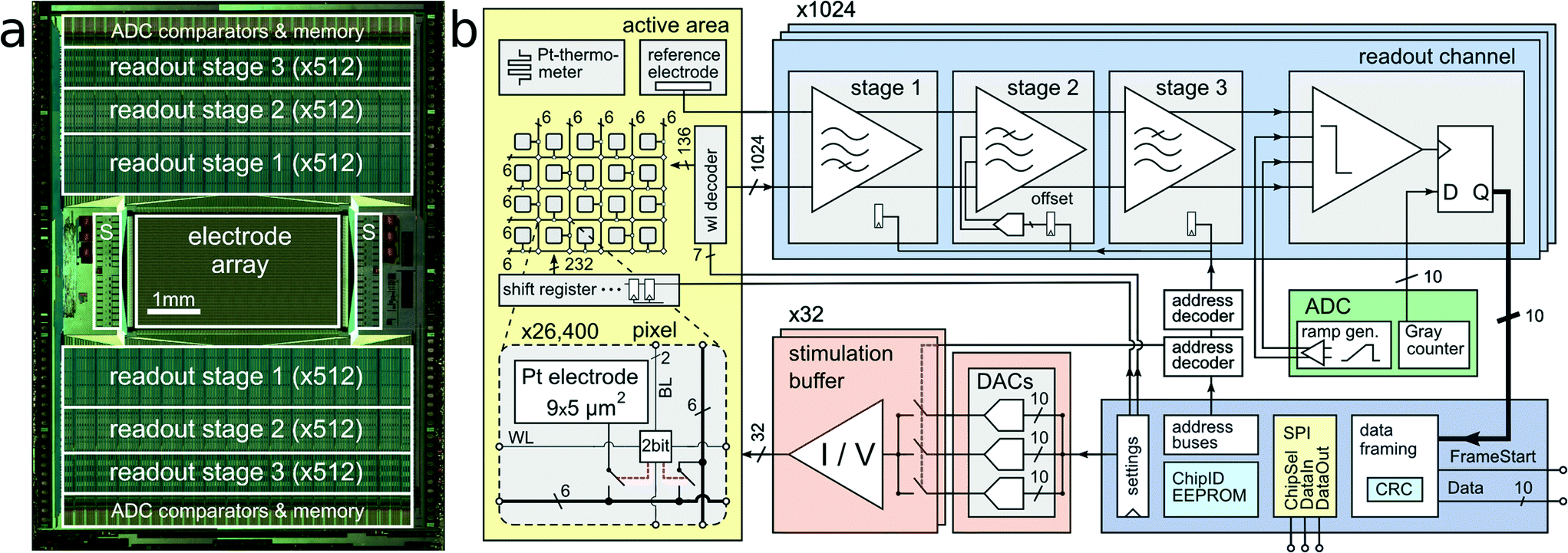Fig. 1 System Architecture. CMOS MEA system architecture. (a) Micrograph of the CMOS device (10.1 × 7.6 mm²). The 1024 readout channels are arranged at the top and bottom of the 3.85 × 2.10 mm² microelectrode array. The 32 stimulation units (S) are located on the left and right side of the array. (b) Block diagram of the implemented circuitry. A close-up view into the electrode array shows details of one individual pixel including the 9.3 × 5.45 μm² platinum electrode, a two-bit SRAM cell, and two switches.

2.2. Reconfiguration of the microelectrode array

To accommodate different experimental needs, the microelectrode array can be reconfigured within milliseconds. Fig. 2A shows a subset of the array with its electrodes, switches, and wires used to implement the flexible routing. Fig. 2B shows an example mathematical graph representing a drastically simplified part of the array. In this example, three out of the four available electrodes can be connected to readout channels by closing the appropriate switches. As it is impossible to manually determine the best routing paths from all 1024 selected electrodes to the respective readout units, a custom software algorithm has been developed to calculate optimum routing paths and to set the states for all 86 000 switches. Fig. 2C shows a flowchart of the steps involved to record from a certain, freely selectable subset of all available 26 400 electrodes. First, custom software maps the electrode array into a mathematical graph. Each electrode and wire is represented as a node in the graph, and each switch as an arc between two nodes. Then, an integer linear programming (ILP) algorithm optimizes a max-flow min-cost problem,¹⁴i.e. the number of readable recording electrodes is maximized (max-flow), while the number of used resources (switches, wires) is minimized (min-cost). To this end, the algorithm needs to apply a set of constraints, such as (i) each assigned electrode is a signal source, (ii) every available readout channel is a signal sink, and (iii) no more than one routing signal is allowed per node and arc. Once the algorithm found a solution to the constrained optimization, the serial interface of the CMOS MEA is employed to download the configuration to all switches in the chip, and neural data can be recorded. As depicted in Fig. 2C, a typical experimental session consists of iterative execution of the flowchart. The operator chooses initial sets of 1024 electrodes either randomly, according to some scanning scheme, or manually. Neural activity, as captured by these electrodes, is analyzed for measures such as firing rate, signal amplitude, or response characteristics to a given stimulus. Once an overview over the preparation under study has been attained, the most appropriate electrodes can be selected, and the actual experiment can be performed.

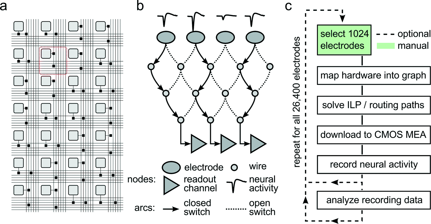Fig. 2 Reconfigurable Electrode Array. (a) Schematic of the wiring in a part of the array. Light gray squares represent electrodes; black squares represent switches controlled by SRAM cells. Buses of 6 horizontal and 6 vertical wires are arranged per row and column. The area highlighted with the red square corresponds to one pixel unit. (b) Simplified mathematical graph showing a drastically reduced subset of the array. Three of the four electrodes picking up neural signals are connected through a set of switches and wires to three readout channels by closing the respective switches. (c) Flow chart of a typical experiment run. After choosing 1024 out of 26 400 electrodes, the hardware is mapped into a mathematical graph representing the array. Within this graph, an integer linear programming (ILP) max-flow min-cost problem is solved, and optimal signal routing paths are determined. The corresponding switch configuration is then downloaded into the CMOS MEA, and neural activity can be recorded. Once the activity on all 26 400 electrodes has been analyzed, best-suited recording electrode candidates are determined so that the final experiment can be performed.

2.3. Readout and stimulation units

The 1024 readout channels consist of three amplification stages, providing a programmable total gain of up to 78 dB for the accommodation of a wide range of different signal amplitudes.²² The first stage includes a 1.4 pF input capacitance to provide AC coupling and to filter the offset and low-frequency drift in the electrode potential. The second stage implements a digitally-assisted offset compensation scheme to cancel output offset of the first stage. Anti-aliasing low-pass filtering is implemented through the second and third stage. The input-referred readout noise in the action-potential signal band (300 Hz–10 kHz) is 2.4 μV_rms.²² The amplified and band-pass filtered signals are sampled at 20 kHz with 1024 on-chip 10 bit analog-to-digital converters (ADCs). By digitizing the signals on-chip, digital codes can be multiplexed and transmitted off-chip. In contrast to analog signals, digital signals are very resistant to interference noise that may be caused by nearby measurement equipment or culturing incubators. Each packet of data is protected with a cyclic redundancy code (CRC) checksum to detect data corruption.

A total of 32 stimulation buffers,²⁵ capable of providing arbitrary voltage or current-controlled stimulation waveforms, resides at the left and right side of the sensing area. The stimulation units can be connected to an arbitrary selection of electrodes. Multiple electrodes can be connected together to form larger stimulation patches.^26,27 Although featuring low static power consumption, the buffers can drive loads as large as 11 nF, while a signal rise time below 50 μs for a 2.5 V step is preserved. This load corresponds roughly to 200–500 connected Pt bright electrodes or 5–20 Pt black electrodes, depending on the electrode impedances. In current mode, the deliverable current can be as large as 50 μA at a resolution of 2 nA. Three digital-to-analog converters (DACs) can be programmed to provide independent stimulus waveforms. In an alternative stimulation mode, the output voltages of the DACs can be kept fixed, but the input of the stimulation buffers can be switched between the available DAC voltages. This allows for implementation of independent waveforms for each of the 32 stimulation units with arbitrary phase timing but fixed voltage or current amplitudes.

2.4. Fabrication and post-processing

The CMOS device has been fabricated in a 0.35 μm technology (2P4M) and post-processed at wafer level to (i) produce long-term stable Pt-electrodes and to (ii) further enhance the passivation layer to protect the circuitry against culturing media. During the same post-processing step, a Pt-thermoresistor was fabricated, which allows for measuring the temperature at the chip surface during experiments in order to strictly preserve physiological temperatures. The post-processing steps have been abstracted before.²⁴ In brief, Si₃N₄ was first deposited by means of plasma-enhanced chemical vapor deposition (PECVD), and the pads and electrodes were subsequently re-opened through reactive-ion etching (RIE). Next, TiW (50 nm), for promotion of adhesion, and Pt (270 nm), as electrode material, were ion-beam-deposited and then patterned by using an ion-beam etching step. A 4-layer 1.6 μm-thick passivation stack, consisting of alternating SiO₂ and Si₃N₄ layers was deposited by PECVD; finally, a re-opening of the platinum electrodes was achieved through an RIE step. The top-metal layer below the electrode openings is free of features to provide flat structures and to ensure good connectivity and adhesion of the post-processed Pt-layer.

2.5. Chip preparation

Once the wafers were post-processed, and diced, the chips were bonded to custom printed-circuit boards (PCBs). A biocompatible epoxy was used to encapsulate the bond-wires and PCB tracks in order to protect them from the culturing media. This packaging makes the devices stable and suitable for experiments involving culturing of cells over periods of months. To reduce the impedance of the microelectrodes, Pt-black was electrochemically deposited on the electrodes.¹⁹ The on-chip Pt thermoresistor was calibrated by using a two-point calibration procedure.

2.6. Culturing and imaging

Cortical neurons and glia were grown over the CMOS-MEA to test the performance of the system. Briefly, E18 rat cortices were dissociated enzymatically in trypsin (Invitrogen), followed by mechanical trituration. A layer of poly(ethyleneimine) (Sigma) and a layer of laminin (Sigma) were used to adhere between 20 k to 40 k cells. The media used for plating consisted of 850 μL of Neurobasal, supplemented with 10% horse serum (HyClone), 0.5 mM GlutaMAX (Invitrogen), and 2% B27 (Invitrogen). After 24 hours, the plating medium was changed to growth medium: 850 μL of DMEM (Invitrogen), supplemented with 10% horse serum, 0.5 mM GlutaMAX, and 1 mM sodium pyruvate (Invitrogen). Prior to experimentation, cultures matured for 3 to 4 weeks, and experiments were conducted inside an incubator to control environmental conditions (36.5 °C and 5% CO₂). All animal handling protocols were approved by the Basel Stadt veterinary office according to Swiss federal laws on animal welfare. To visualize clusters of neurons grown on the HD-MEA, cells were sparsely transfected with a human synapsin I promoter driving DsRedExpress from the Callaway laboratory, Salk Institute, La Jolla, USA (Addgene plasmid 22909) with Lipofectamine 2000 (Invitrogen 11668). After experiments, cell cultures were fixed in 4% paraformaldehyde (Invitrogen) in PBS (phosphate-buffered saline; Sigma) and permeabilized (0.25% Triton X-100 (Sigma) in PBS), Then, the primary antibody to MAP2 (Abcam ab5392) diluted 1 : 500 in PBS with 1% BSA (bovine serum albumin; Sigma) and 0.1% Tween20 was added and left overnight at 4 °C on a shaker at low speed. The secondary antibody containing Alexa Fluor 647 (Invitrogen A21449), diluted to 1 : 200, was applied for 1 h at room temperature in the dark. A Leica DM6000 FS microscope with a 10× long-working-distance objective lens and a Leica DFC 345 FX camera were used to collect images at room temperature. For further details see ref. 23.

2.7. Single cell identification

The extracellular field of a single neuron can be measured up to tens of micrometers away from the soma.^20,28,29 Due to the densely spaced microelectrodes, multiple electrodes usually record the extracellular field potential of a single neuron. Exploiting this fact facilitates the task of assigning extracellularly recorded field potentials to individual neurons.³⁰ As it is computationally intractable to process all thousand channels at once, prior to analysis, the recording electrodes were clustered into groups of up to 16 neighboring electrodes. Spike identification and sorting was performed within these electrode groups, and, subsequently, spike trains of neurons, present in more than one electrode group, were merged based on (i) the Euclidean distance of the extracellular field potential and (ii) the similarity in the spike train time stamps.

Analysis within these electrode groups was carried out as follows. First, traces were band-pass filtered (300–2500 Hz). Then, spikes were identified when the negative voltage peak crossed a threshold, which was set to 4.5 times the standard deviation of the noise.³¹ Spike waveforms were cut out from 2 ms before to 3 ms after reaching their negative peak values on all electrodes of the corresponding group. The cut out traces were first up-sampled 8 times and subsequently aligned with respect to the negative peaks. Principal component analysis (PCA) was performed on the concatenated waveforms to reduce dimensionality of the data, and principal components were clustered by fitting a mixture of Gaussians through an expectation maximization (EM) algorithm as further described in ref. 32.

Once spike times for the individual neurons have been identified, the spike triggered average on all 1024 recorded electrodes (the extracellular electrical signature of one single neuron on all electrodes, on which it is visible, is sometimes denoted electric ‘footprint’) has been estimated by re-extracting and averaging the events from the raw data, which now have been band-pass filtered between 100 and 9000 Hz.

It frequently happens that two nearby neurons spike simultaneously, or very shortly after one another, causing overlapping electrical fields. Depending on the exact relative timing of the overlaps, this causes significant distortions to the recorded traces, and spike sorting becomes more difficult. However, unless the cells are active multiple times with the exact same relative timing, the overlaps will not produce the same compound waveform shape so that during the clustering process, these overlaps can be identified as outliers and discarded. Although there have been techniques developed to address this problem,^33–36 we decided to discard such events, as we were primarily interested in reconstructing the accurate extracellular electric footprint for every single cell and not in reconstructing the exact spike train for each cell. To this end, we computed the spike-triggered-average (STA) for single cells by taking the median over many time-aligned AP occurrences.

When long recordings were analyzed (on the range of tens of minutes to hours), a slightly different approach was used, since overlaps may occur frequently, to the extent that they form their own clusters and are erroneously identified as neurons. For the first few minutes of the recordings, the clustering process described above was applied, but then template matching was performed on the remaining data using the extracted electrical footprints as templates.^35,37

2.8. Identification of axonal arbors

The large sensing area and the large amount of microelectrodes allow for electrical identification of potentially large axonal arbors of single cells. Compared to the relatively large amplitudes of extracellular somatic signals (hundreds of μV), signals from axons are very small and often buried in noise (on the order of a few μV's). Therefore, a special technique must be applied in order to reveal such axonal signals. Once, somatic APs of a single cell have been identified through spike sorting, the axonal arbor of this cell can be reconstructed by spike-triggered-averaging of multiple instances of single axonal APs to reduce the influence of uncorrelated noise. Since not all electrodes can be read out at the same time, a scheme to scan through all electrodes is employed. To this end, a few electrodes recording with the best available signal-to-noise ratio (SNR) are used to continuously record from the soma of a given cell, while the remaining recording channels are used to consecutively scan the activity on all other electrodes. Template matching is performed on the fixed electrodes to identify spike timings of the single cell (see 2.7. Single cell identification). Averaging of all identified events reduces noise and helps to reveal electrical signals originating from small neurites far away from the cell body.²³ For robustness and to eliminate outliers (in this case spikes from other neurons), the median was calculated instead of the mean.

3. Results

We used the HD-MEA to analyze information processing in neuronal networks at different scales of spatial resolution. First, a coarse overview of the neuronal network was obtained. At the next level of higher resolution, a smaller area of the network was examined and analyzed in more detail, revealing many spatially overlapping different single neurons. A fluorescence image of a MAP2 staining of the respective cell culture provided the correlations between electrical recordings and optical imaging. Finally, at the highest resolution, subcellular properties of single neurons were identified, showing axonal arbors spanning over all the active sensing area. Furthermore, precise and spatially-confined electrical stimulation was used to evoke electrical activity of individual axons. When an axon is stimulated, the elicited AP can be tracked as it propagates down the axonal arbor through several different branches. As outlined above, the HD-MEA architecture is designed in a way that electrodes are not equipped with individually dedicated amplifiers. Instead an arbitrary subset out of all electrodes is connected to 1024 low-noise readout channels (including amplifiers), residing at the periphery of the sensing area (see Methods). Thus, before information processing in the neural network can be analyzed, the most suitable electrodes must be chosen; the respective selection strategies are described below.

3.1. Network-wide analysis

Recording of electrical activity on all electrodes gives an activity map of the biological preparation and reveals areas with no activity, which can be excluded from further analysis. Initially, dense blocks of electrodes were scanned through the array, and activity was recorded for 2.5 minutes for each such block. To cover all 26 400 electrodes, 27 different configurations were used. After the data were recorded, a threshold-crossing algorithm, applied offline, identified spike timings. In Fig. 3A the neural spiking activity on each electrode is presented on a logarithmic gray scale between 1 Hz and 2 kHz. Areas with no detectable electrical signals can be excluded from further analysis, and the available recording channels can be focused on areas exhibiting activity.

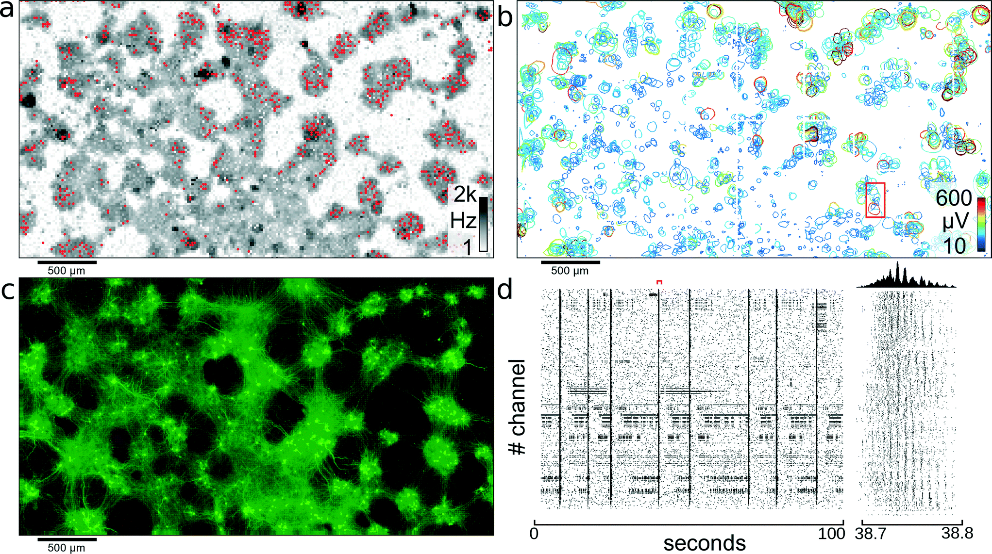Fig. 3 Network of cortical neurons. Network of cortical neurons grown over the 3.85 × 2.10 mm² microelectrode array area. (a) Average action potential firing rate as measured by each electrode and displayed on a logarithmic gray-scale between 1 Hz and 2 kHz. Red dots indicate the 1024 electrodes used for recording of the network activity. (b) Representation of all 2000 individual single cells that could be identified through spike sorting the signals of high-density electrode configurations. A circle is drawn around each detectable cell and indicates the level where the amplitude of the electrical signals of a cell footprint exceed −4.5 standard deviations of the electrode noise. The color-coding indicates the maximum amplitude of the most negative peak for each neuronal electrical footprint. The red rectangle indicates the area used for further analysis shown in Fig. 4. (c) Fluorescence image of transfected cells. Transfection ratio was around 5% (according to the manufacturer) of all cells; therefore, only a subset of all cells lights up; clearly visible are clusters of neurons and the tracks of interconnecting neurite bundles. (d) Raster plot of 100 seconds of activity for all 1024 recording channels. The red marker indicates the time period shown in the close up view to the right. Between 38.7 and 38.8 seconds, waves of activity propagate through the network. The histogram at the top shows the number of spikes per time bin.

Once areas with active neurons have been identified, the readout channels can be connected to electrodes most suitable for recording from many neurons in parallel. To generate a suitable recording electrode selection, one of two strategies was applied: In the more time-consuming strategy, single electrodes were carefully chosen to record reliably and in parallel from as many cells as possible. The electrodes were selected in a way to maximize the number of recorded neurons and to minimize redundancies in recordings. This approach requires careful analysis of all neuronal footprints and is computationally intensive. It is further described in section 3.4.

Alternatively, a more heuristic approach can be employed by first estimating the cell density from the activity map. In the presence of dense neurons with spatially overlapping extracellular field potentials, a single electrode picks up electrical activity from more than one neuron. Thus electrodes recording high activity and many APs short after each other, i.e., within less than a single cells refractory period (between 1.5 ms and 3 ms), indicate overlapping extracellular action potentials from multiple cells and may indicate areas with high cell densities. Previous experiments done with tetrodes³⁸ have shown that the spike-sorting yield of locally-dense electrode clusters is markedly better than distributing the readout sites into isolated spots. Because the extracellular electric fields rapidly decay in amplitude with increasing distance,³⁹ the fields of neighboring neurons can be distinguished on nearby electrodes, which helps to capture shapes of field potentials of individual neurons more reliably. To maximize the number of recorded single cells, active recording sites have, therefore, been arranged in several hundred locally-dense, globally-sparse electrode clusters.

The red dots in Fig. 3A represent a configuration of locally-dense, globally-sparse distributed clusters of 1024 electrodes used to record from the neuronal network. Following application of this configuration of electrodes, 1105 cells could be identified after spike sorting. Fig. 3D shows a raster plot of 100 seconds recorded with the 1024 electrodes highlighted in Fig. 3A.

3.2. Single-cell analysis

The previously recorded data obtained from blocks of densely-spaced electrodes was spike-sorted to yield not only temporal information about individual neuron spike timings but also the spatial distribution of single-cell extracellular electrical action potentials, termed “footprints,” as described in the section 2.6. Two distinct temporal network states were observed: one with the majority of cells spiking sparsely in time and weakly correlated with each other; the second state was one in which most cells of one cell cluster were bursting and thus were synchronously active. It is difficult to identify single-cell activity, when all neurons are active at the same time, due to their strongly overlapping electrical fields. To reduce the number of overlapping extracellular action potentials and to, thereby, obtain best sorting performance, only time periods with no or small cell-cluster bursts involving no more than a few tens of cells were analyzed (for identification of bursts, see also ref. 40). For visualizing extracellular AP footprints (Fig. 3B), a contour line was plotted in regions where the electrical activity signals of that cell exceeded 4.5 standard deviations of the noise threshold, to indicate electrodes capable of picking up the signal from that cell. With spike sorting, an estimated total of 2000 neurons could be identified in the culture shown in Fig. 3. From Fig. 3A–C, it is apparent that cells in this culture aggregated into clusters of densely-packed neurons. The activity map, as well as the spike-sorted overview (Fig. 3A, B) matches closely to the fluorescence image of the culture in Fig. 3C. Furthermore, it can be seen from Fig. 3C that these islands of cell clusters are interconnected with tracks of neuronal processes; see also section 3.5.

3.3. Correlation of electrical activity with fluorescence imaging

To prove correct identification of single cells, the electrical activity data have been compared to the fluorescence image of a MAP2 immunostaining of the respective cell culture. Through staining, the cell bodies and dendrites become fluorescent and can be imaged on top of the array with a microscope. As can be seen in Fig. 4A, the spike-triggered averages (STA) of the action potentials of a single cell align with the fluorescently marked cell bodies. The largest voltage signal is not necessarily at the cell body but offset towards the axon initial segment, which has the highest ion-channel density. The cell in the upper left corner (STAs plotted in green) exhibits action potentials with very large amplitudes. The largest peak-to-peak signal of this cell has an amplitude of almost 3 mV and is recorded on the electrode labeled with “5”. The very same same cell exhibits electrical activity with large amplitudes even at electrodes quite distant from the soma (more than 180 μm), which can be assigned to the axon of this cell (see section 3.5).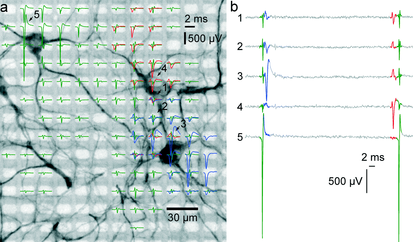

Fig. 4 Electrical activity superimposed to a MAP2 staining of the neurons. (a) The electrical activity of three neurons is superimposed to a fluorescence image of a MAP2 staining of the cell culture in the respective area. Spike-triggered averages of signals from 3 different neurons over 50 trials are drawn in green, red and blue. Averaged traces are only displayed for electrodes with a peak-to-peak signal amplitude exceeding 50 μV. The activity of a single cell can be recorded on fairly distant electrodes. Particularly, the green traces exhibit signals of very large amplitudes (almost 3 mV peak-to-peak), and putative axonal signals can be seen at electrodes at more than 180 μm distance from the soma. The red set of signal traces exhibits the largest negative peak value in the 4th row, 9th column and features signals with negative peaks in the first row and signals with positive peaks in the 8th row. (b) Sixty milliseconds of raw data as recorded on the five electrodes marked with arrows and numbers in (a). At least three individual spikes can be identified in this period. The activities of the single cells can be recorded through multiple electrodes.

3.4. Determination of best recording electrodes

A procedure to determine the smallest number of necessary electrodes that are optimal for recording from a given set of neurons was developed. In order to simultaneously record from as many neurons as possible, only electrodes strictly needed to properly identify neurons should be allocated for recording and connected to readout channels. When zooming into the culture of Fig. 3 within the area marked with the red frame in Fig. 3B, electrical footprints of at least five overlapping cells are revealed. Fig. 5A shows these five cells with their STA signal on all electrodes where the amplitude of their action potential exceeds the 4.5 std noise threshold. As the neurons in this cell cluster exhibit overlapping electrical activity in space as well as in time, proper cell identification is difficult, and spike-sorting algorithms are challenged. However, spike sorting is most effective when the activity of a cell is recorded on many electrodes, which is made possible by the high spatial electrode density. Each of the five neurons could be detected, on average, on 45 electrodes on which their signal amplitudes exceeded 4.5 std noise levels. For two neighboring neurons (e.g., the red and the green shapes in Fig. 5A), the recorded signals might differ only marginally on a single electrode. But by taking together many small differences from many electrodes, the cumulative difference gets more significant, and activities of these two cells can more reliably be differentiated.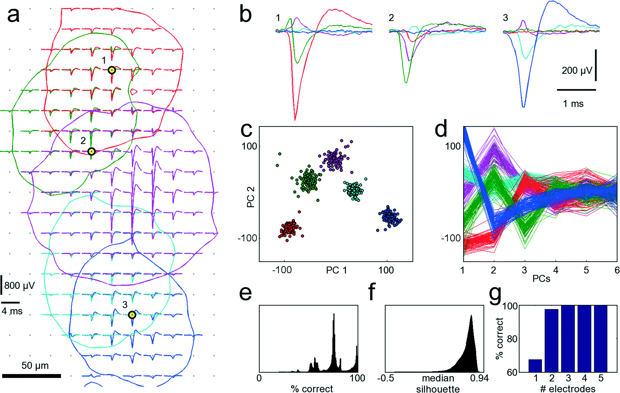

Fig. 5 Single-cell resolution. The electrical activity of five neurons has been identified and spike-sorted with 209 electrodes. Subsequently, the performances of all combinations of selecting 3 out of 209 electrodes were analyzed in terms of correctly classified APs. Refer to text for a detailed discussion of the procedure. (a) Spike-triggered averages of five identified neurons with overlapping electrical footprints. For each neuron, a circle is drawn where the amplitude of their electrical signal exceeds a threshold of 4.5 standard deviations of the noise level. Black-yellow circles indicate the three electrodes yielding best sorting performance. (b) Spike-triggered average waveforms recorded with the three electrodes marked in (a). (c) Principal component (PC) projection of 500 AP waveforms recorded with the three electrodes marked in (a). The PC projection is used for clustering. (d) First six PCs of all 500 AP waveforms. Color coding of the neurons is identical for all subfigures. (e) Distribution of performances for all 1.45 million tested electrode combinations. A considerable fraction yields more than 95% correct classifications. (f) Distribution of medians of the silhouette coefficients for all 1.45 million tested electrode combinations for the clustered waveforms as in (c). (g) Comparison of the best achievable spike-sorting performance for different numbers of electrodes. With just one electrode, only about 65% of all APs can be correctly classified. With three electrodes and more, the performance saturates at 100%, thus three electrodes chosen at suitable spots are sufficient to reliably record and distinguish the signals from the five neurons displayed in (a). The supplementary material contains more figures that show the analysis for one, two, four and five out of 209 selected electrodes (see ESI,† SF1_a–SF1_e).

Thus, in a first step, all 209 electrodes below these five neurons were used for recording AP activity. Since AP events were recorded with approx. 45 electrodes per neuron, spike sorting could be performed with relatively high reliability, and its results were considered the ground truth for further analysis.^30,41 The waveforms for 100 AP occurrences per neuron and for each electrode were aligned in time, and data between 2 ms before and 3 ms after the AP peak were cut out. Next, all 1.45 million different combinations of choosing 3 out of 209 electrodes were sampled, and their spike-sorting performances were analyzed. To this end, the 100 AP waveforms for each neuron together with 100 noise waveforms (to accommodate for the case of no AP) were taken from each electrode. Next, PCA was performed on the concatenated waveforms to reduce dimensionality and, subsequently, the first 10 PCs were clustered with the k-means algorithm.⁴² Since it is a priori known that there should be 6 different clusters, i.e., the 5 neurons plus the white noise, k-means was performed with k = 6. As the k-means algorithm has a stochastic component, which can mistakenly lead to correct classifications by chance, the clustering was repeated 10 times, and the most frequently occurring solution was chosen. For each electrode combinations, the number of correctly classified AP waveforms that could be clustered was analyzed. If multiple electrode combinations performed equally well, the one that also provided the best cluster separation, as quantified by the median of the silhouette coefficients,⁴³ was chosen. Fig. 5A indicates the three best-performing electrodes, marked with black and yellow circles. In Fig. 5B, the STA for all five neurons on these three electrodes is shown. It is apparent that the shapes provide good separability, which can also be seen from the clustering results in the PCA space in Fig. 5C, D. This procedure was repeated iteratively by choosing 1, 2, 4 or 5 out of 209 electrodes. Instead of analyzing the clustering results in the PCA space, other measures, such as Fisher information, could be used.⁴⁴Fig. 5G shows the best achievable spike-sorting performance for the different numbers of selected electrodes. It is no surprise that the electrodes yielding the largest peak signals for the respective neurons are chosen upon searching for the 5 optimally placed electrodes (see ESI† Fig. SF1_e). This selection result is in accordance with intuition. It is worth noting, however, that upon choosing a subset of electrodes to identify different cells, in particular, when the electrode number is smaller than the number of neurons to be distinguished, the electrodes that record the largest spike amplitudes are not necessarily chosen; rather, those that collectively provide best separability for all neurons are selected.

With 3 electrodes and more, performance saturates at 100% correctly classified APs, and, therefore, the three electrodes indicated in Fig. 5A are sufficient to record the activities of these five neurons. Hence, it is possible to reliably record from a number of neurons that exceeds the number of available electrodes. Figures with more clustering and electrode selection results are shown in the ESI,† SF1.

3.5. Subcellular-resolution analysis

The minute extracellular signals of the axonal arbor of a single cell can be identified and tracked over the large sensing area of the HD-MEA by spike-triggered averaging of the electrical signals. The method described in section 2.8 was applied, where three electrodes capturing the electrical signal with the largest amplitude for a defined cell were kept fixed, and all other array electrodes were scanned through. Between 30 and 50 AP occurrences were recorded per configuration. Large axonal arbors of single cells could be revealed with this method; Fig. 6A and B show the axonal arbor of one single cell. The axonal arbor spans over almost the entire electrode array, and signals of individual axons can be recorded at up to 3 mm distance from the soma and up to 6 ms after the somatic spike. The availability of multiple electrodes around one axon enables averaging in space in addition to averaging in time. Averaging in the time-domain, as done previously to get the STAs, reveals the spatial arrangements of axonal segments through their electrical footprints. Once the spatial arrangement of the axon has been identified, spatial averaging can be used to reduce the noise of an individual axonal AP (amplitudes of 5–20 μV). Fig. 6E shows 25 traces recorded with electrodes that pick up signals of an axonal branch. The spike-triggered average in the time domain (50 averages) is shown at the right, and a single axonal AP buried in noise at the left. Temporal alignment of the signals from neighbored electrodes with respect to the negative peak value of the axonal AP (Fig. 6F left) and subsequent averaging of all signals (Fig. 6F right) enhances the correlated signal amplitude much more than that of the uncorrelated noise.

Fig. 6 Axonal arbors. Identified axonal arbor of a single cell revealing subcellular features up to more than 2 mm distance from the cell body. (a) All electrodes capturing activity attributed to a single neuron. Color-coding indicates the time of arrival of the AP at the respective electrode. It takes 6 ms for the AP to arrive at the left-most visible axonal segment. A video showing the AP propagation down the axonal arbor is available as ESI† Video SM1. (b) The same neuron and electrodes as in (a), this time showing the amplitude of the most negative peak on a logarithmic color-scale. Its putative soma is inside the box indicated with (c). (c) And (d) spike-triggered averages (30 to 50 averages) of the electrical footprint from two areas of the array as indicated in (b). The scale bars of (d) apply to the signals in (c) and (d). (e) Left: 25 traces from electrodes that detect axonal signals. Spike-triggered averaging (50 APs) reduces noise. Right: traces from the same electrodes showing a single axonal AP hidden in the noise. Red dots indicate the timing of the negative peak. (f) Left: all 25 recording traces of one axonal AP overlaid and aligned in time with respect to the negative peak. Right: spatial averaging of traces aligned in time with respect to the negative peak from multiple neighbored electrodes that detect axonal signals improves axonal AP detectability. The Gaussian-like distribution of the noise is shown, and dashed red lines indicate one standard deviation. Green lines indicate 4.5 standard deviations, the detection threshold. (g) The signal amplitude (green curve, right ordinate) scales linearly with an increasing number of electrodes (#electrodes), whereas the noise floor (blue curve, left ordinate) scales with a square root function. The dashed blue curve indicates the scaling of uncorrelated noise. When summing signals from more than four electrodes, the signal amplitude is more than 4.5 times larger (70 μV) than the standard deviation of the noise (15 μV), so that the signals can be considered detectable. See text for a more detailed discussion.

Fig. 6G shows how the signal amplitude increases linearly, while the standard deviation (std) of the noise increases according to a square-root function of the number of summed time-aligned electrode signals. The time-aligned summation is shown in Fig. 6G to display the linear and square-root dependence, whereas the time-aligned average is shown in Fig. 6E and F. In the particular case displayed in Fig. 6G, the use of more than four electrodes makes the signal amplitude exceed 4.5 std of the noise floor and thus makes it detectable. Under the assumption of statistically independent noise, the power of noise on multiple electrodes adds up linearly with the number of used electrodes, whereas the power of the signal features a square-law dependence.⁴⁵ Noise is typically not statistically independent on nearby electrodes (blue curve). However, by whitening the signals prior to summing them, uncorrelated noise can be approximated.³⁴ The dashed blue curve shows how uncorrelated noise would add up in the ideal case.

3.6. Electrical stimulation of axonal tissue

Electrical stimulation of neural tissue through single microelectrodes reliably elicits time-locked action potentials. Fig. 7 shows a configuration where 841 electrodes were chosen below an axonal segment. The electrode denoted with “stimulation site” in Fig. 7A was repeatedly stimulated with biphasic, first positive then negative voltage pulses of 200 μs duration per phase and ±400 mV amplitude. Such a stimulation pulse activates the axonal segment passing across the microelectrode so that an action potential is initiated and travels down the axon. It takes 2.1 ms to travel 1.56 mm, i.e., the average propagation speed for this axon is 0.74 m s⁻¹. The propagation speed has been calculated by dividing the linear distance between two electrodes marked with the red-white circle by the time it takes for the negative peak of the AP to travel that same distance. While the measured speed is highest close to the stimulation site (0.9 m s⁻¹) it decays with increasing distances down to 0.4 m s⁻¹. The measured values are in agreement with reported propagation speeds for unmyelinated axons.⁴⁶ In Fig. 7B, a stereotypical positive-first waveform of the traveling axonal AP can be seen at three different time points. Close to electrode 3, around 800 μm from the stimulation site, the axon splits into two branches, an upper and a lower branch. Interestingly, it appears that the AP in the upper branch travels faster than in the lower one. At t₂ = 1.0 ms the AP in the upper branch is further advanced than that in the lower branch. It is unclear, however, whether this difference in propagation velocity is due to, e.g., a longer axon, i.e., an extra loop, which is not visible, or whether it is due to differences in axonal diameters⁴⁷ or other properties. The cause for this difference in propagation velocity cannot clearly be identified without further analysis, such as high-resolution imaging of the axon geometry. An analysis directly on the device is, however, very challenging due to the nontransparent nature and corrugated surface of the CMOS substrate (super-resolution optical methods are not applicable).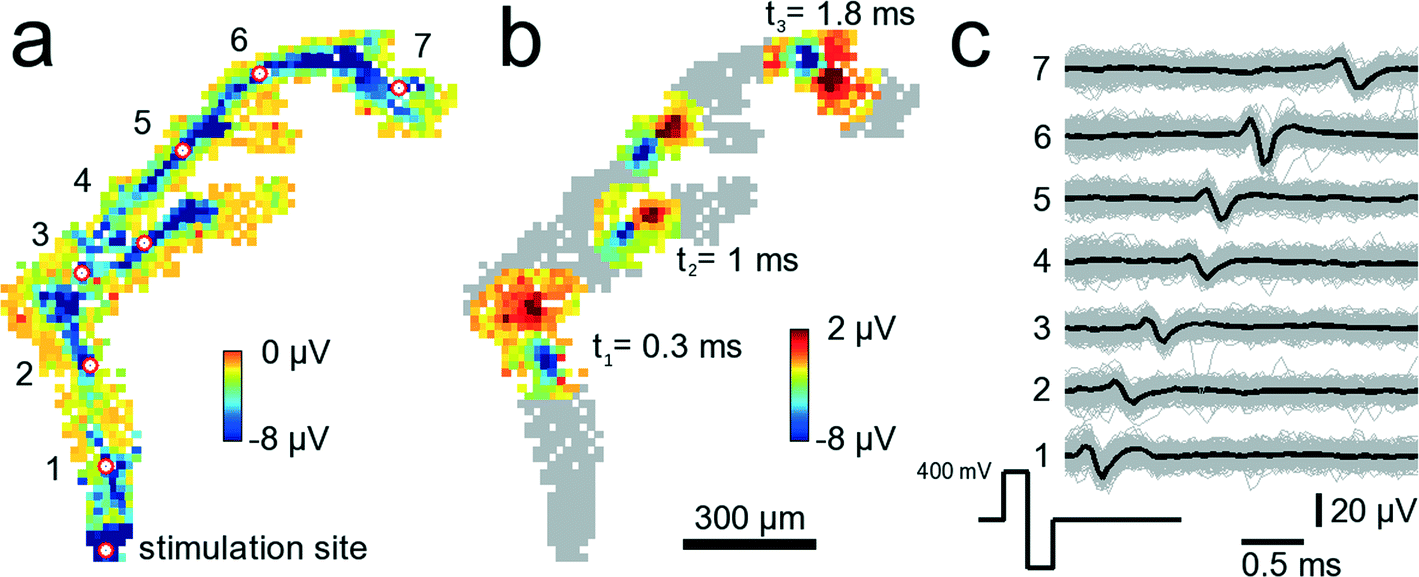

Fig. 7 Tracking of stimulated signals in axonal arbors. 841 electrodes below an axonal arbor record the stimulation-induced axonal propagation of an AP. A video showing the propagating AP is available as ESI† Video SM3. (a) The site at the bottom denoted stimulation site has been stimulated 200 times with biphasic 300 mV voltage pulses at 300 ms inter-stimulus intervals. Each square shows the average AP minimum value on a clipped color scale over the 200 trials for each recorded electrode within 3 ms after stimulation. The red circles with white fillings indicate electrodes for which voltage traces are shown in (c). Close to the electrode indicated with 3, the axon splits into two different branches. (b) Same neuron and electrodes as in (a). This time, the propagating AP is shown at three different time points, t₁ = 0.3, t₂ = 1.0 and t₃ = 1.8 ms after stimulation occurred. At t₂, the AP has already passed the branch point such that the AP can be seen in both branches. (c) Voltage traces from the 7 electrodes marked with the red-white circles in (a). Shown are voltage traces for single trials (gray) and the median over all trials (black).

The amplitude of the axonal signal in Fig. 7 was larger than 20 μV in some locations and varied along the axon. These variations could be a consequence of biological material, such as another neuron or glia residing between the axon and the electrode, the effect of which would locally reduce signal amplitudes. Also, such material could reside on top of the axon towards the solution and then enhance signal amplitudes by spatially confining the area through which charge-carrying ions could spread.

3.7. Microelectrode characterization

A series of measurements was performed to characterize the microelectrodes and to quantify electrode-to-electrode variations, as well as their stability over time. Impedance values for 300 randomly selected bright Pt and 300 Pt-black electrodes were measured at 1 kHz (see section 2.4 and 2.5 for how Pt-black electrodes are fabricated). At this frequency, the electrodes can be approximated as being purely capacitive.⁴⁸ The electrode capacitances were determined via the measured impedance at 1 kHz according to the formula: Z_imp = 1/(jωC_el), where Z_imp is the measured impedance, C_el is the determined electrode capacitance, and ω is the angular frequency. Using the on-chip stimulation buffers, a sinusoidal current with amplitudes of ±20 nA was applied to bright Pt electrodes and ±200 nA to Pt-black electrodes. On-chip amplifiers were used to measure the voltage drop across the electrodes. The capacitances of bright Pt electrodes were found to be 45.0 ± 10 pF (mean ± std). Capacitance values of Pt-black electrodes amounted to 2.0 ± 0.26 nF (mean ± std). Measurements for a device with Pt-black electrodes, after being exposed to more than 5 months of cell culturing were shifted to 0.65 ± 0.27 nF (mean ± std) (Fig. 8). The impedance did not measurably change over tens of thousands of stimulations. Finally, electrodes survive long periods of cell culturing. Two devices exposed to more than 5 months of cell culturing were submerged in PBS, and a test signal was applied to a counter Pt-electrode held in the PBS. All electrodes recorded the test signal without degraded amplitude as compared to an unused device.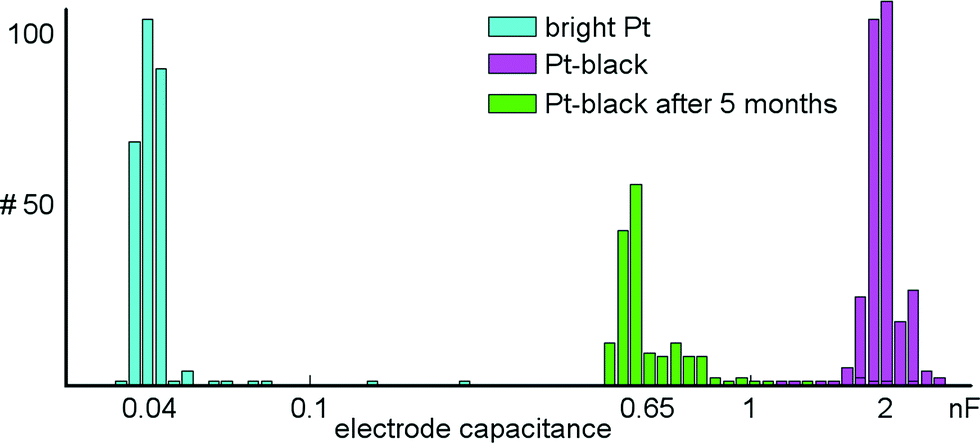

Fig. 8 Electrode impedance measurements. Shown are the capacitances of 300 randomly selected bright Pt and Pt-black electrodes based on impedance measurements at 1 kHz. The capacitances are plotted on a logarithmic scale. The capacitances of Pt-black electrodes are about 50 times larger than those of the bright Pt electrodes. The distribution shown in green indicates the capacitances for 300 randomly selected electrodes after 5 months of culturing cells on top of them.

4. Discussion and outlook

We presented a CMOS based HD-MEA capable of, at the same time, recording from neuronal networks with hundreds of cells as well as of capturing subtle subcellular signal details from the axonal arbor of single neurons. This performance is made possible by the inherent system flexibility as well as a large number of parallel low-noise readout and stimulation channels.

We think that the system presented here constitutes a favorable combination of high signal quality and high spatial resolution. The number of 1024 channels that can be simultaneously read out is on the same order of magnitude albeit somewhat lower than that of other devices,^12,13,16 whereas the noise in the recordings is considerably lower (2.4 μV_rms in the action-potential band between 300 Hz and 10 kHz). The low noise and high recording quality together with the large dynamic range of the on-chip ADCs, enable not only tracking of the spreading of multiple APs over many different neurons, but, at the same time, also their propagation along the axonal arbor of a single cell.

Compared to previous implementations, such as^49,50 and, in particular,¹⁴ the switch matrix was advanced through the following features: instead of a few long wires running across the whole array, we implemented hundreds of thousands of comparably short routing wires (420 μm average length) in order to massively increase the number of potential routing paths for all array electrodes; moreover, the number of wires per line and column was increased to 6 horizontal and 6 vertical wires, and the number of switches was increased to two per electrode, enabled through the use of 0.35 μm CMOS technology , to achieve a highly flexible electrode to readout-circuitry routing. This flexible switch matrix structure together with the large overall number of available array electrodes enables the device to record the activity of neuronal networks consisting of hundreds of cells by employing globally-sparse, locally-dense configurations of recording electrodes. The electrode array supports operation in three different modes, or arbitrary combinations thereof: (i) locally-dense electrode clusters of up to 23 × 23 (529) contiguous electrodes at arbitrary positions massively improve the separation of spatially overlapping extracellular action potentials; (ii) sparse distribution of such clusters or single electrodes across the whole array allows for recording from many cells in distant regions at the same time; (iii) by recruiting all available electrodes below a certain axonal arbor, it is also possible to observe how cellular parameters, such as signal propagation velocities,^7,51–53 fluctuate over time, and how axons spatially move during the course of an experiment. Signals originating from axons are often on the same order of magnitude as the noise floor, making it difficult to detect such signals without averaging. However, temporal averaging only gives a population average over all observed spikes and does not permit studying single APs. Spatial averaging, enabled by the high spatial resolution of electrodes and the low noise, can be employed to study temporal changes in propagation velocity or branch point failures^46,54 of single APs. Besides spatial averaging, more sophisticated signal processing algorithms will be developed in the future in an effort to more reliably detect axonal signals.

Concerning the number of readout channels, it has to be noted that the data volume produced by HD-MEAs can be enormous and amounts to, e.g., 1.4 GB per minute for reading from 1024 channels at 20 kHz. An option to deselect electrodes with no relevant information can be very useful, as exclusion of non-active areas saves disk storage space, as well as data analysis time.

To make most efficient use of available resources, recording channels can be allocated only to electrodes in the vicinity of neurons that are producing signals relevant to the ongoing investigation.

Electrode-to-electrode variations in impedance values were found to be very small over the whole array. All 26 400 microelectrodes could be reliably used even after long periods of culturing cells on top. The shift in impedance values for Pt-black electrodes, which had cells on top for more than 5 months, can be due to various reasons: (i) mechanical damage to the fine Pt-black structures upon washing/cleaning the chips, (ii) residual adhesion or protein layers from the culturing that cover the dendritic Pt structures, or (iii) cell debris, all of which would cause an increase in impedance.

Recording the dynamics of large networks at a spatiotemporal resolution sufficient to simultaneously resolve individual APs of single cells is challenging for conventional techniques and arrays. For example, single cells can be resolved upon imaging calcium activity. However, in addition to being phototoxic, the temporal resolution is limited making it difficult to capture the waveform shape and the temporal-dynamics of single APs (in the range of kHz).⁵⁵ Genetically targeted all-optical electrophysiology methods have recently emerged that provide better temporal and spatial resolution and hold the promise of all-optical electrophysiology,⁵⁶ but experiments at resolutions necessary for studying axonal signals have, however, not been demonstrated to date. Intracellular electrical recordings carried out with patch-clamp are well-suited for the study of cellular or subcellular properties of individual neurons; they can be used to record and resolve synaptic currents with high SNR, but fail at recording from populations of more than a few cells. Extracellular recordings based on passive MEAs on the other hand, can access many neurons at the same time with temporal resolutions high enough to resolve individual action potentials. However, due to the comparably large electrode spacing (>30 μm), it is often the case that not all neurons in a population can be captured, that the resolution of overlapping neurons is difficult, or that, for example, axonal signals cannot be reliably detected. Recent developments also include small arrays of mushroom shaped electrodes^57,58 or nanowires on electrodes,⁵⁹ which can be engulfed by the cell membrane and allow for pseudo-intracellular recordings. The arrays currently feature, however, only tens of simultaneously readable recording sites.

Although extracellular recordings are better suited to investigate network-wide activity than recordings with patch-clamp setups, inferences about neuronal plasticity in extracellular recordings are inherently more difficult, as the postsynaptic potentials are not directly measurable.⁶⁰ Exploiting, e.g., homeostasis in neuronal networks,⁶¹ measuring changes in network functional connectivity estimations could be used as a proxy for quantifying changes in postsynaptic potentials and network plasticity.⁶² This approach, will, however, require access to potentially every cell in a network.

Possible future research with a configurable HD-MEA, as used in this study, may include constraining a few hundred neurons to grow on the active area of the HD-MEA. By capturing the full activity of this complete neuronal population, under-sampling of the network is avoided, and the number of hidden variables is reduced. In this case, the inference of network parameters, such as functional connectivity, is significantly more robust.⁶³ Care has to be taken, however, when interpreting data recorded on such a network-wide scale: spikes originating from the same cell but recorded on different neighboring electrodes might falsely show up as strongly correlated cells, or two or more cells might be recognized as a single cell, thus underestimating connectivity. Spike sorting of such datasets prior to analyzing network activity is a crucial step, since failing to do so can distort or bias the data.

Contributions

Experimental design, data analysis and software/hardware development was done by J.M.; J.M., M.B., Y.C., P.L., developed CMOS circuitry; A.St. did post-processing of CMOS wafers; technical support was provided by A.Sh., V.V., D.J.B., R.D. and U.F.; experimental support was provided by D.J.B., M.R., I.L.J. and M.F.; J.M., D.J.B., U.F., Y.C., I.L.J. and A.H. wrote the manuscript; supervised the project: A.H. and D.J.B.

Acknowledgements

The authors would like to thank Jörg Rothe for support and consulting while developing the electronic components for the setup, David Jäckel for help with the imaging, Dr. Felix Franke for helpful discussion on spike-sorting algorithms and Dr. Thomas Russell for culturing assistance. This work was supported by the ERC Advanced Grant “NeuroCMOS” under contract number AdG 267351. M. Radivojevic and D. J. Bakkum received funding support from the Swiss National Foundation through an Ambizione Grant (PZ00P3_132245).

References

1. A. P. Alivisatos, A. M. Andrews, E. S. Boyden, M. Chun, G. M. Church, K. Deisseroth, J. P. Donoghue, S. E. Fraser, J. Lippincott-Schwartz and L. L. Looger, ACS Nano, 2013, 7, 1850–1866.
2. A. H. Marblestone, B. M. Zamft, Y. G. Maguire, M. G. Shapiro, T. R. Cybulski, J. I. Glaser, D. Amodei, P. B. Stranges, R. Kalhor, D. A. Dalrymple, D. Seo, E. Alon, M. M. Maharbiz, J. M. Carmena, J. M. Rabaey, E. S. Boyden, G. M. Church and K. P. Kording, Front. Comput. Neurosci., 2013, 7, 137,  DOI:10.3389/fncom.2013.00137.
3. F. Gerhard, T. Kispersky, G. J. Gutierrez, E. Marder, M. Kramer and U. Eden, PLoS Comput. Biol., 2013, 9, e1003138.
4. P. J. Sjöström, E. A. Rancz, A. Roth and M. Häusser, Physiol. Rev., 2008, 88, 769–840.
5. W. Zhang and D. J. Linden, Nat. Rev. Neurosci., 2003, 4, 885–900.
6. D. Debanne, Nat. Rev. Neurosci., 2004, 5, 304–316.
7. D. J. Bakkum, Z. C. Chao and S. M. Potter, PLoS One, 2008, 3, e2088.
8. E. M. Izhikevich, Neural Comput., 2006, 18, 245–282.
9. H. Alle and J. R. Geiger, Science, 2006, 311, 1290–1293.
10. G. W. Gross, B. K. Rhoades, H. M. E. Azzazy and W. Ming-Chi, Biosens. Bioelectron., 1995, 10, 553–567.
11. A. Stett, U. Egert, E. Guenther, F. Hofmann, T. Meyer, W. Nisch and H. Haemmerle, Anal. Bioanal. Chem., 2003, V377, 486–495.
12. L. Berdondini, K. Imfeld, A. Maccione, M. Tedesco, S. Neukom, M. Koudelka-Hep and S. Martinoia, Lab Chip, 2009, 9, 2644–2651.
13. B. Eversmann, M. Jenkner, F. Hofmann, C. Paulus, R. Brederlow, B. Holzapfl, P. Fromherz, M. Merz, M. Brenner, M. Schreiter, R. Gabl, K. Plehnert, M. Steinhauser, G. Eckstein, D. Schmitt-Landsiedel and R. Thewes, IEEE J. Solid-State Circuits, 2003, 38, 2306–2317.
14. U. Frey, J. Sedivy, F. Heer, R. Pedron, M. Ballini, J. Mueller, D. Bakkum, S. Hafizovic, F. D. Faraci, F. Greve, K.-U. Kirstein and A. Hierlemann, IEEE J. Solid-State Circuits, 2010, 45, 467–482,  DOI:10.1109/JSSC.2009.2035196.
15. A. Hierlemann, U. Frey, S. Hafizovic and F. Heer, Proc. IEEE, 2011, 99, 252–284.
16. G. Bertotti, D. Velychko, N. Dodel, S. Keil, D. Wolansky, B. Tillak, et al., A CMOS-based sensor array for in-vitro neural tissue interfacing with 4225 recording sites and 1024 stimulation sites, in Biomedical Circuits and Systems Conference (BioCAS), Lausanne, 1199, 2014.
17. R. Huys, D. Braeken, D. Jans, A. Stassen, N. Collaert, J. Wouters, J. Loo, S. Severi, F. Vleugels and G. Callewaert, Lab Chip, 2012, 12, 1274–1280.
18. B. Eversmann, A. Lambacher, T. Gerling, A. Kunze, P. Fromherz and R. Thewes, A neural tissue interfacing chip for in-vitro applications with 32k recording/stimulation channels on an active area of 2.6 mm², 2011 Proceedings ESSCIRC, Helsinki, 2011, pp. 211–214.
19. F. Heer, S. Hafizovic, W. Franks, A. Blau, C. Ziegler and A. Hierlemann, IEEE J. Solid-State Circuits, 2006, 41, 1620–1629.
20. U. Frey, U. Egert, F. Heer, S. Hafizovic and A. Hierlemann, Biosens. Bioelectron., 2009, 24, 2191–2198.
21. H. Wässle, Nat. Rev. Neurosci., 2004, 5, 747–757.
22. M. Ballini, J. Muller, P. Livi, Y. Chen, U. Frey, A. Stettler, A. Shadmani, V. Viswam, I. L. Jones and D. Jackel, 2014.
23. D. J. Bakkum, U. Frey, M. Radivojevic, T. L. Russell, J. Müller, M. Fiscella, H. Takahashi and A. Hierlemann, Nat. Commun., 2013, 4, 2181,  DOI:10.1038/ncomms3181.
24. J. Müller, M. Ballini, P. Livi, Y. Chen, A. Shadmani, U. Frey, I. Jones, M. Fiscella, M. Radivojevic, D. Bakkum, A. Stettler, F. Heer and A. Hierlemann, Conferring Flexibility and Reconfigurability to a 26'400 Microelectrode CMOS Array for High Throughput Neural Recordings, Proceedings of the 17th IEEE International Conference on Solid-State Sensors, Actuators and Microsystems, Transducers, Barcelona, Spain, 2013, pp. 744–747.
25. P. Livi, F. Heer, U. Frey, D. J. Bakkum and A. Hierlemann, IEEE Trans. Biomed. Circuits Syst., 2010, 4, 372–378.
26. M. R. Behrend, A. K. Ahuja, M. S. Humayun, R. H. Chow and J. D. Weiland, IEEE Trans. Neural. Syst. Rehabil. Eng., 2011, 19, 436–442.
27. M. Eickenscheidt and G. Zeck, J. Neural. Eng., 2014, 11, 036006.
28. F. Mechler, J. D. Victor, I. Ohiorhenuan, A. M. Schmid and Q. Hu, J. Neurophysiol., 2011, 106, 828.
29. C. Gold, D. A. Henze, C. Koch and G. Buzsáki, J. Neurophysiol., 2006, 95, 3113–3128.
30. F. Franke, D. Jackel, J. Dragas, J. Muller, M. Radivojevic, B. Douglas and A. Hierlemann, Front. Neural Circuits, 2012, 6, 105,  DOI:10.3389/fncir.2012.00105.
31. M. S. Lewicki, Network: Computation in Neural Systems, 1998, 53–78.
32. S. N. Kadir, D. F. Goodman and K. D. Harris, 2013, arXiv preprint arXiv:1309.2848.
33. J. W. Pillow, J. Shlens, E. Chichilnisky and E. P. Simoncelli, PLoS One, 2013, 8, e62123.
34. C. Pouzat, O. Mazor and G. Laurent, J. Neurosci. Methods, 2002, 122, 43–57.
35. F. Franke, M. Natora, C. Boucsein, M. H. Munk and K. Obermayer, J. Comput. Neurosci., 2010, 29, 127–148.
36. D. Jackel, U. Frey, M. Fiscella, F. Franke and A. Hierlemann, J. Neurophysiol., 2012, 108, 334–348.
37. R. Vollgraf and K. Obermayer, IEEE Signal Process Lett., 2006, 13, 121–124.
38. C. M. Gray, P. E. Maldonado, M. Wilson and B. McNaughton, J. Neurosci. Methods, 1995, 63, 43–54.
39. W. Rall, Biophys. J., 1962, 2, 145–167.
40. D. J. Bakkum, M. Radivojevic, U. Frey, F. Franke, A. Hierlemann and H. Takahashi, Front. Comput. Neurosci., 2013, 7, 193.
41. I. D. Ruz and S. R. Schultz, J. Neurosci. Methods, 2014, 233, 115–128.
42. J. MacQueen, Some methods for classification and analysis of multivariate observations, Proceedings of the fifth Berkeley symposium on mathematical statistics and probability, 1967, vol. 1, no. 14.
43. P. J. Rousseeuw, J. Comput. Appl. Math., 1987, 20, 53–65.
44. T. R. Cybulski, J. I. Glaser, A. H. Marblestone, B. M. Zamft, E. S. Boyden, G. M. Church and K. P. Kording, 2014, arXiv preprint arXiv:1402.3375.
45. H. Ku, Precision Measurement and Calibration, NBS SP 3D0, 1969, vol. 1, pp. 331–341.
46. D. Debanne, E. Campanac, A. Bialowas, E. Carlier and G. Alcaraz, Physiol. Rev., 2011, 91, 555–602.
47. A. Schierwagen and M. Ohme, in COLLECTIVE DYNAMICS: TOPICS ON COMPETITION AND COOPERATION IN THE BIOSCIENCES: A Selection of Papers in the Proceedings of the BIOCOMP2007 International Conference, ed. A. Buonocore, E. Pirozzi and L. M. Ricciardi, 2008, vol. 1028, Vietri sul Mare, Italy, pp. 98–112.
48. W. Franks, I. Schenker, P. Schmutz and A. Hierlemann, IEEE Trans. Biomed. Eng., 2005, 52, 1295–1302.
49. K. Seidl, S. Herwik, T. Torfs, H. P. Neves, O. Paul and P. Ruther, J. Microelectromech. Syst., 2011, 20, 1439–1448.
50. C. M. Lopez, A. Andrei, S. Mitra, M. Welkenhuysen, W. Eberle, C. Bartic, R. Puers, R. F. Yazicioglu and G. G. Gielen, IEEE J. Solid-State Circuits, 2014, 49, 248–261.
51. D. Bakkum, U. Frey, M. Radivojevic, T. Russell, J. Müller, M. Fiscella, H. Takahashi and A. Hierlemann, Nat. Commun., 2013, 4.
52. M. Greschner, G. D. Field, P. H. Li, M. L. Schiff, J. L. Gauthier, D. Ahn, A. Sher, A. M. Litke and E. Chichilnisky, J. Neurosci., 2014, 34, 3597–3606.
53. G. Zeck, A. Lambacher and P. Fromherz, PLoS One, 2011, 6, e20810.
54. Y.-T. Kim, K. Karthikeyan, S. Chirvi and D. P. Davé, Lab Chip, 2009, 9, 2576–2581.
55. C. Grienberger and A. Konnerth, Neuron, 2012, 73, 862–885.
56. D. R. Hochbaum, Y. Zhao, S. L. Farhi, N. Klapoetke, C. A. Werley, V. Kapoor, P. Zou, J. M. Kralj, D. Maclaurin and N. Smedemark-Margulies, Nat. Methods, 2014, 825–833.
57. M. E. Spira, D. Kamber, A. Dormann, A. Cohen, C. Bartic, G. Borghs, J. P. M. Langedijk, S. Yitzchaik, K. Shabthai and J. Shappir, TRANSDUCERS '07 & Eurosensors XXI. 2007 14th International Conference on Solid-State Sensors, Actuators and Microsystems, 2007, pp. 1247–1250.
58. A. Hai and M. E. Spira, Lab Chip, 2012, 12, 2865–2873.
59. J. T. Robinson, M. Jorgolli, A. K. Shalek, M.-H. Yoon, R. S. Gertner and H. Park, Nat. Nanotechnol., 2012, 7, 180–184.
60. J. Müller, D. J. Bakkum and A. Hierlemann, Front. Neural Circuits, 2013, 6, 121,  DOI:10.3389/fncir.2012.00121.
61. G. G. Turrigiano and S. B. Nelson, Curr. Opin. Neurobiol., 2000, 10, 358–364.
62. I. H. Stevenson and K. Koerding, Inferring spike-timing-dependent plasticity from spike train data, in Advances in Neural Information Processing Systems, 2011, pp. 2582–2590.
63. F. Gerhard, G. Pipa, B. Lima, S. Neuenschwander and W. Gerstner, Front. Comput. Neurosci., 2011, 5, 4.

---

Footnote

† Electronic supplementary information (ESI) available: See DOI: 10.1039/c5lc00133a

---