Source apportionment of polycyclic aromatic hydrocarbons in PM2.5 using positive matrix factorization modeling in Shanghai, China

Abstract

Providing quantitative information on the sources of PM2.5-bound polycyclic aromatic hydrocarbons (PAHs) in urban regions is vital to establish effective abatement strategies for air pollution in a megacity. In this study, based on a year data set from October 2011 to August 2012, the sources of PM2.5-bound 16 USEPA priority PAHs (16 PAHs) in Shanghai, a megacity in China, were apportioned by positive matrix factorization (PMF) modeling. The average concentrations (in ng m⁻³) of 16 PAHs in PM2.5 in the fall, winter, spring and summer were 20.5 ± 18.2, 27.2 ± 24.0, 13.7 ± 7.7 and 6.4 ± 8.1, respectively, with an annual average of 16.9 ± 9.0. The source apportionment by PMF indicated that coal burning (30.5%) and gasoline engine emission (29.0%) were the two major sources of PAHs in the PM2.5 in Shanghai, followed by diesel engine emission (17.5%), air-surface exchange (11.9%) and biomass burning (11.1%). The highest source contributor for PAHs in the fall and winter was gasoline engine emission (36.7%) and coal burning (41.9%), respectively; while in the spring and summer, it was diesel engine emission that contributed the most (52.1% and 43.5%, respectively). It was suggested that there was a higher contribution of PAHs from engine emissions in 2011–2012 compared with those in 2002–2003. The major sources apportioned by PMF complemented well with this of using diagnostic ratios, suggesting a convincing identification of sources for the PM2.5-bound 16 PAHs in a megacity.

---

Environmental impact

This is the first study that quantitatively apportioned the sources of PM2.5-bound polycyclic aromatic hydrocarbons (PAHs) in Shanghai using positive matrix factorization (PMF) modeling. Five distinct source categories, namely, gasoline engine emission, diesel engine emission, coal burning, biomass burning, and air-surface exchange were identified. The major sources apportioned by PMF complemented well with that of using diagnostic ratios, suggesting a convincing identification of sources for the PM2.5-bound 16 PAHs in a megacity. This work, we believe, can provide insight into the identification of organic contamination in the megacity in China, and perhaps in the world.

Introduction

Polycyclic aromatic hydrocarbons (PAHs), a family of organic compounds that consist of fused aromatic rings, are byproducts of the incomplete combustion of organic materials. They mainly originate from anthropogenic sources, such as pyrogenic processes including domestic and industrial coal combustion, biomass burning and vehicle emissions.^1,2 Due to their carcinogenic or mutagenic properties, PAHs have been of great concern and a highlight of air pollution research. PAHs were ubiquitous in the atmosphere, and had side effects on human health through inhalation or ingestion.^3,4 Therefore, understanding the sources of the PAHs in the atmosphere is very important for controlling the air quality and reducing human exposure to these toxic pollutants.

In recent years, air quality research has focused on fine particles (i.e., PM2.5, aerodynamic diameter less than 2.5 μm) due to their strong effects on atmospheric visibility, human health and global climate. Shanghai, the largest city in China by population (i.e., ∼24 million in 2013), is one of the global financial centers and a transport hub with the world's busiest container port. According to the monitored data, the PM2.5 pollution in Shanghai deteriorated in the recent decade, and its significant role in the air quality of Shanghai has been a source of great concern for researchers. For example, Hou et al. (2011) reported the carbonaceous pollutants in PM2.5 in Shanghai in 2006–2007, and assessed their implication on heavy haze formation.⁵ Huang et al. (2012) observed three typically episodic hazes associated with 2009 PM2.5 in Shanghai, and found that the chemical composition of PM2.5 played a key role in air quality.⁶ Furthermore, there have been studies emphasizing specific components, such as PAHs, in the PM2.5 of Shanghai. Feng et al. (2006) measured the composition and sources of organic matter in PM2.5, and found that engine exhausts made a prominent contribution to PAHs in urban areas.⁷ Gu et al. (2010) presented the occurrence and compositions of PAHs based on over two years of PM2.5 samples, and revealed the sources of petroleum and coal/biomass combustion for PAHs.⁸ These studies provided qualitative information on PAH sources, and implied that PAHs played a significant role in the air quality of Shanghai. It should be noted that, although the air quality of Shanghai has been ameliorated since the mid-1990s, fine particles (i.e., PM2.5) and the associated organic fraction still remain priority pollutants in the atmosphere.⁹ Therefore, in order to more effectively abate the organic contamination and especially the PAH fraction in the PM2.5 in Shanghai, it is necessary to quantitatively apportion the sources of these pollutants. However, to the best of our knowledge, no work has been published on the quantitative apportionment of PAH sources in the atmosphere of Shanghai. In this study, 72 PM2.5 samples from October 2011 to August 2012 were collected at an urban site in Shanghai. The objectives of this work are to examine the seasonal variation of PAH occurrence and composition, and to apportion the sources of the PAHs using positive matrix factorization (PMF) modeling.

Materials and methods

Sampling site and sample collection

The sampling site (31.3°N, 121.5°E) is located on the roof of the no. 4 teaching building, a five-storey building with a height of ∼15 m, on the campus of Fudan University in the northeast of Shanghai. This site is a super air quality monitoring station of Fudan University in Shanghai.⁶ This sampling location is approximately 1 km away from the Wujiaochang shopping center, one of the four sub-centers in Shanghai. The closest industry to this site is mainly located to the southeast and northwest, and it is about 10.5 km distant.¹⁰ Two roadways with heavy traffic, Guoding road and Handan road, surround a major part of the campus. The resident population in this area (Yangpu District) is about 1.3 million (http://www.yprk.com/).

The PM2.5 samples were collected by an aerosol sampler (Guangzhou Mingye Huanbao Technology Company) with quartz filters (20 × 25 cm², 2500 QAT, PALL, USA) at a flow rate of 18 m³ h⁻¹. The sampler began to collect samples at 9:00 am on day one and stopped at 8:30 am the following day, ensuring the duration time for a sample was about 23.5 h. A total of 72 PM2.5 samples were taken during 24 Oct. to 16 Nov. 2011 (fall, n = 20), 24 Dec. 2011–11 Jan. 2012 (winter, n = 18), 29 Mar.–28 Apr. 2012 (spring, n = 19) and 24 Jul.–12 Aug. 2012 (summer, n = 15). Each paired sampling campaign consisted of a 23.5 h sampling, starting at 9:00 am on the first day to 8:30 am the following day. There were at least two parallel operational sampling blanks in each season. Sample media were prepared as follows: the filters were wrapped in aluminum foil and baked together at 450 °C for 4 h to remove residual organic contaminants; they were then sealed in marked valve bags and stored in the laboratory prior to sample collection. All post-sampling filters were stored at −20 °C for later analysis.

Sample analysis for PAHs

The analytical procedure for PAHs has been described previously.^11,12 In brief, half of each PM2.5 sampling filter was used for Soxhelt extraction. For the recovery rate, a mixture of compounds including deuterated naphthalene (Nap-d₈, m/z 136), deuterated acenaphthene (Ace-d₁₀, m/z 164), deuterated phenanthrene (Phe-d₁₀, m/z 188), deuterated chryene (Chr-d₁₂, m/z 240) and deuterated perylene (Per-d₁₂, m/z 264) was added into all the samples prior to extraction. The extraction was for 48 hours using dichloromethane (DCM) as the extracting solvent. The total extracts were concentrated to about 5 ml using a rotary evaporator. Then, the solvent was exchanged to hexane (HEX) and samples were further concentrated to about 2 ml with a stream of highly purified N₂. The concentrated extracts were sequentially purified in the chromatography column filled with 3 cm deactivated alumina (Al₂O₃), 3 cm silica gel (SiO₂) and 1 cm anhydrous sodium sulfate (Na₂SO₄) and eluted with 20 ml of DCM/HEX (1 : 1, v:v). A sample vial (2 ml) was prepared for the final concentrated extract and hexamethylbenzene (HMB) was used as the internal standard to quantify the PAHs. The PAHs were USEPA priority PAHs (16 PAHs). The standard 16 PAHs and five deuterated PAHs were purchased from Accu Standard, Inc. (USA). The 16 targeted PAHs were as follows: 2-ring, naphthalene (Nap); 3-ring, acenaphthylene (Ac), acenaphthene (Ace), fluorene (Fl), phenanthrene (Phe), anthracene (Ant); 4-ring, fluoranthene (Flu), pyrene (Pyr), benzo[a]anthracene (BaA), chrysene (Chr); 5-ring, benzo[b]fluoranthene (BbF), benzo[k]fluoranthene (BkF), benzo[a]pyrene (BaP), dibenzo[a,h]anthracene (DBA); and 6-ring: indeno[1,2,3-cd] pyrene (IP), benzo[ghi]perylene (BghiP). For the GC-MS analysis, all the samples were injected with HMB and then concentrated to about 200 μl. The GC-MSD (Agilent GC 6890 N coupled with 5975C MSD, equipped with a DB5-MS column, 30 m × 0.25 mm × 0.25 μm) had helium as the carrier gas. The GC operating processing was held at 60 °C for 2 min, ramped to 290 °C at 3 °C min⁻¹ and held for 20 min. The sample was injected split-less with the injector temperature at 290 °C. The post-run time was 5 min with the oven temperature at 310 °C.

Sample analysis for organic carbon (OC) and elemental carbon (EC)

The OC and EC fractions were detected by the IMPROVE thermal/optical reflectance (TOR) method which was initiated by the Desert Research Institute (DRI).¹³ A 0.544 cm² area of each sample was punched to analyze the targeted carbon fractions including four OC (OC1, OC2, OC3, and OC4), three EC (EC1, EC2, and EC3) fractions, and a pyrolyzed carbon fraction (OP). OC1, OC2, OC3, and OC4 were formed in a helium atmosphere at temperatures of 140 °C, 280 °C, 480 °C and 580 °C, respectively. EC1, EC2 and EC3 were formed in a 2% oxygen/98% helium atmosphere under the temperature of 580 °C, 740 °C and 840 °C, respectively. OC was operationally defined as the total carbon in the sample when heated up to 550 °C in a 100% helium atmosphere. EC was defined as all carbon when heated up to 800 °C in an atmosphere of 2% oxygen and 98% helium after removal of OC. OP was determined as reflecting a transmittance laser light attained its original intensity after oxygen was added to the analysis atmosphere. Therefore, OC and EC were obtained as OC1 + OC2 + OC3 + OC4 + OP and EC1 + EC2 + EC3 − OP, respectively.

QA/QC

Organic reagents (DCM, HEX) extracting PAHs were purchased from the Shanghai ANPEL Scientific Instrument Company (HPLC grade, purity: 95%). All vessels were first rinsed with hot potassium dichromate–sulfuric acid lotion, then left overnight and washed using 18.2 MΩ Milli-Q water. After packing these vessels with aluminum foil, they were put in muffle furnace at 450 °C for 4 hours. All utensils were rinsed twice with reagents before use. The mean recoveries for all PM2.5 samples were 71% ± 12% for Nap-d₈, 78% ± 10% for Ace-d₁₀, 91% ± 13% for Phe-d₁₀, 103% ± 15% for Chr-d₁₂ and 105% ± 12% for Per-d₁₂, respectively. Procedural blanks, standard-spiked blanks and matrices were analyzed. The targeted 16 PAH compounds were not detected in the procedural blank; the PAH recoveries of the standard-spiked matrix ranged from 85% to 95%; and the paired duplicate samples agreed to within 15% of the measured values (n = 10). Sample results were displayed as a blank correction by subtracting an average blank from each sample. The reported concentrations here are not recovery corrected. The QA/QC procedures of OC and EC were: 10.56 μg of sucrose was used to calibrate the analyzer every day with a difference <6% for the recovery rate. One replicate analysis was conducted for every ten samples. The differences determined from the replicate analyses were <5% for OC and EC. Two parallel blank filters were analyzed following the same procedures in each season for the samples. Results were corrected with respect to the average blank concentrations. The detection limits for OC and EC were below 1.0 μg m⁻³.

PMF modeling

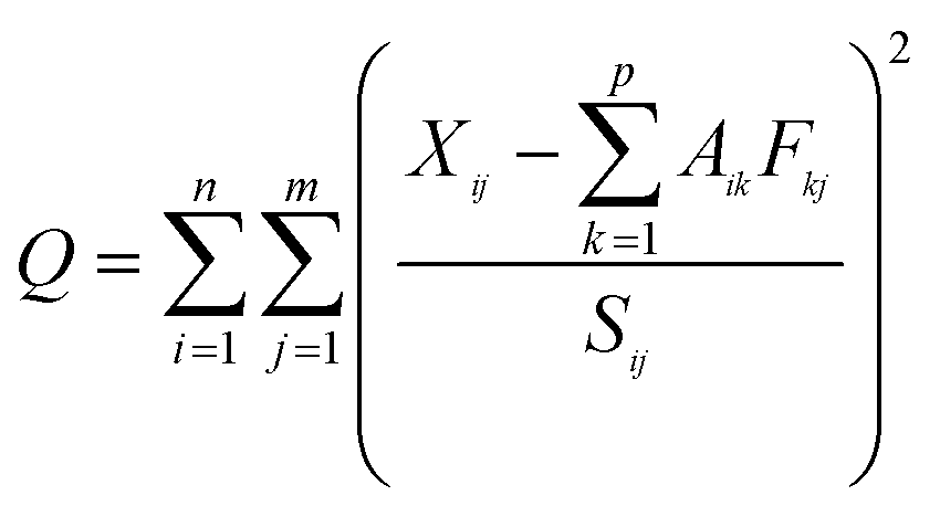
Detailed descriptions of the PMF application on source apportionment are given at EPA PMF 3.0 Fundamentals & User Guide (http://www.epa.gov/heasd/products/pmf). In brief, the PMF model is based on the following equation:
where X_ij is the concentration of the j^th congener in the i^th sample of the original data set; A_ik is the contribution of the k^th factor to the i^th sample; F_kj is the fraction of the k^th factor arising from congener j; and R_ij is the residual between the measured X_ij and the estimated X_ij using p principal components.
where S_ij is the uncertainty of the j^th congener in the i^th sample of the original data set containing m congeners and n samples. Q is the weighted sum of squares of differences between the PMF output and the original data set. One of the objectives of PMF analysis is to minimize the Q value. Importantly, there is a critical step in PMF analysis to determine the number of factors. A detailed determination for such types of “factors” is described elsewhere.¹⁴ In this study, the number of factors from 3 to 7 was examined with the optimal number of factors determined from the slope of the Q value versus the number of factors. For each run, the stability and reliability of the output were checked based on the Q value, residual analysis and correlation coefficients between observed and predicted concentrations. Finally, a 5-factor solution, which gave the most stable results and easily interpretable factors compared with the source factors apportioned by Wang et al. (2014),¹² was chosen for the data sets. Before the analysis, a data set that included unique uncertainty values of each data point was created and inserted into the model. An uncertainty of 20% for each PAH dataset was used in this study according to Mai et al. (2003).¹¹

Results and discussion

Occurrence and composition of PAHs

Seasonal variation of the concentrations of 16 PAHs (in ng m⁻³) in the PM2.5 samples during the sampling period are shown in Fig. 1. An obvious seasonal variation of the 16 PAH concentrations could be observed, with the highest in the winter (27.2 ± 24.0), the lowest in the summer (6.4 ± 8.1), and intermediate values in the fall and spring, (20.5 ± 18.2 and 13.7 ± 7.7 respectively). The concentrations of the individual 16 PAHs are given in Table S1.† The annual average concentration of the 16 PAHs was 16.9 ± 9.0. As shown in Table 1, the mean value of the PAHs in PM2.5 in Shanghai was lower than that of the northern cities in China, such as Beijing,¹⁵ Harbin¹⁶ and Qingdao,¹⁷ by a factor of 3–5, but comparable with those of Guangzhou¹⁸ and Xiamen,¹⁹ two coastal cities in South China. However, compared to studies conducted in urban areas around the world, such as Los Angeles²⁰ and London,²¹ the concentrations of the PAHs in PM2.5 in Shanghai were much higher.

Fig. 1 Seasonal variation of concentrations of 16 PAH in PM2.5 in Shanghai.

Table 1 Comparison of the concentrations of PAHs (ng m⁻³) from this study with studies at different areas in the world

Site	Period	Size	PAHs	References
Shanghai	2011, 10 to 2012, 08	PM2.5	16.9	This work
Beijing	2002, 07 to 2003, 01	PM2.5	112.7	15
Harbin	2008, 08 to 2009, 07	TSP	45.0	16
Qingdao	2001, 06 to 2002, 05	TSP	87.5	17
Guangzhou	2001, 04 to 2002, 03	TSP	23.7	18
Xiamen	2008, 10 to 2009, 09	TSP	11.9	19
Los Angeles	2001, 05 to 2002, 07	PM2.5	0.8	20
London	1995, 09 to 1996, 06	TSP	5.8	21

---

According to the properties and sources of the 16 PAHs, they can be classified into 2–3-ring (Nap, Ac, Ace, Fl, Phe, Ant), 4-ring (Flu, Pyr, BaA, Chr), and 5–6-ring PAHs (BbF, BkF, BaP, IP, DBA, BghiP). The seasonal composition patterns for the 16 PAHs are shown in Fig. 2. It can be seen that BbF (7.9–20.4%), BkF (5.2–15.6%), BaP (8.7–12.8%) and BghiP (11.6–14.3%) were the main components. A similar composition pattern over the four seasons can be observed, with the highest contribution from the 5–6-ring (56.4%), followed by the 4-ring (30.6%) and the 2–3-ring PAHs (9.4%). According to Dachs et al. (2002), 2–3-ring PAHs can be formed in the pyrolysis of unburned fossil fuel.²² 4-ring PAHs were abundant in coal combustion¹ and biomass burning.²³ 5–6-ring PAHs mainly originate from high-temperature combustion processes such as vehicular exhaust.²⁴ In this study, the combustion-derived PAHs represented 56.4% of the total PAHs, indicating a prominent contribution from the combusted origins of PAHs. These kinds of composition characteristics for the 16 PAHs in PM2.5 could be caused by various factors, such as meteorological conditions, emission sources and transport paths.^8,25 In this study, we mainly focused on the possible influence of emission sources on the PAH characteristics in PM2.5. This will be further discussed below.

Fig. 2 Seasonal variation of composition patterns of 16 PAHs in PM2.5 in Shanghai.

Associations between 16 PAHs with EC and OC

The concentrations of EC and OC in each sample during the sampling period are shown in Table S2.† Seasonal correlations between the 16 PAHs and EC in PM2.5 are shown in Fig. 3a. Good correlations were observed over the four seasons: fall (R² = 0.84, n = 20, Fig. 3a-1), winter (R² = 0.94, n = 18, Fig. 3a-2), spring (R² = 0.61, n = 19, Fig. 3a-3), and summer (R² = 0.76, n = 15, Fig. 3a-4), respectively. EC usually indicates anthropogenic pollutant sources, such as fossil fuel incomplete combustion, including vehicle emission and coal/biomass burning.²⁶ The relationship of PAHs and EC can be used to identify their possible common combustion sources. Therefore, a fossil fuel combustion source, as stated above, could be a prominent contributor to the 16 PAHs in PM2.5 in Shanghai.

Fig. 3 Seasonal correlations between 16 PAHs with EC and OC in PM2.5 in Shanghai (the extremely high concentration represented by “dark rectangle” in the summer of 2012 was excluded).

The correlations between 16 PAHs and OC are shown in Fig. 3b. As shown, the strongest correlations were in the winter (R² = 0.87, n = 20, Fig. 3b-1), followed by the fall (R² = 0.69, n = 18, Fig. 3b-2) and spring (R² = 0.22, n = 19, Fig. 3b-3). The correlation index in the summer was only 0.02 (n = 15, Fig. 3b-4), much poorer than in the other three seasons. This kind of seasonal difference between PAHs and OC could be attributed to emission sources as well as influence from prevailing meteorological conditions. As suggested by Feng et al. (2009), the OC fractions in PM2.5 of Shanghai, based on four seasonal data sets, were mostly from fossil combustion sources, such as vehicular exhaust and/or coal combustion.⁹ Therefore, the good correlations in the winter and fall indicate that the PAHs were partly associated with vehicular emissions and coal burning. According to Turpin et al. (1995),²⁷ OC can be divided into primary organic carbon and secondary organic carbon (SOC), and a more prominent SOC percentage was revealed in warm seasons than in cold seasons.^26,28 Meteorological conditions in warm seasons, such as a higher frequency of sunny days and more intense solar radiation, could result in a higher photochemical activity.²⁸ In this study, the SOC formation through chemical reactions, such as photolytic oxidation, is a likely cause for the weak correlations between PAHs and OC in the spring and summer. In the summer, higher temperatures and more intense solar radiation could provide more favorable conditions for photochemical activity and SOC production,²⁶ leading to a relatively high availability of gaseous VOC precursors in the atmosphere. Therefore, SOC formation in the summer could be much more prominent than that in the spring, resulting in a rather poor correlation between PAHs and OC.

Sources of PAHs assessed by diagnostic ratios

Diagnostic ratios, namely, ratios of selected PAH concentrations, have been widely used to identify and characterize PAH emission sources. The distributions of the homologues are strongly associated with the formation mechanisms of the carbonaceous aerosols.²⁹ The four diagnostic ratios used in this study were Phe/(Phe + Ant), Flu/(Flu + Pyr), BaA/(BaA + Chr) and IP/(IP + BghiP). The results from this study and those obtained previously by Feng et al. (2006) in the same sampling site are summarized in Table 2.⁷ It can be seen that the ratios of Phe/(Phe + Ant) and Flu/(Flu + Pyr) between these two data sets show almost no difference, with both characterizing coal and biomass burning.³⁰ According to Simcik et al. (1999),³ BaA/(BaA + Chr) > 0.35 indicates pyrolytic sources, and between 0.2 and 0.35 could indicate petrogenic and combustion sources. The ratios of BaA/(BaA + Chr) were 0.29–0.46 (mean: 0.37) in the winter of 2011, while they were 0.26–0.35 (mean: 0.30) in the winter of 2002. A similar trend of BaA/(BaA + Chr) also existed between the summers of 2012 and 2003, which were 0.34–0.47 (mean: 0.38) and 0.28–0.38 (mean: 0.31), respectively. The higher values in both the winter and summer of 2011–2012 than those in 2002–2003 possibly indicate a larger presence of pyrolytic sources such as engine exhausts. IP/(IP + BghiP) > 0.5 signals coal/biomass combustion, and <0.5 indicates engine fuel combustion. In the winter of 2011, IP/(IP + BghiP) values were 0.44–0.48 (mean: 0.45); in the winter of 2003, they were 0.43–0.48 (mean: 0.46), both implying engine fuel combustion sources. In the corresponding summer, the IP/(IP + BghiP) values were 0.40–0.51 (mean: 0.43) and 0.44–0.47 (mean: 0.45), respectively. These indicate a dominance of engine fuel combustion sources. The results could suggest that the contribution of engine fuel (i.e., gasoline and diesel) exhaust for 4-ring PAHs in PM2.5 in Shanghai have been increasing in the recent decade. This could be further supported by the evidence that the number of vehicles in Shanghai significantly increased between 2002 and 2012. There were about 1.3 × 10⁶ vehicles in 2002 while in 2012 there were 2.8 × 10⁶, a twofold increase (Shanghai Statistical Yearbook, 2012).

Table 2 Comparisons of the data set from this study with those obtained previously at the same sampling site with respect to diagnostic ratios. “()” are the mean values

Time	Seasons	Phe/Phe + Ant	Flu/Flu + Pyr	BaA/BaA + Chr	IP/IP + BghiP
2011–2012 (This study)	Fall	0.84–0.91(0.88)	0.50–0.58(0.55)	0.27–0.51(0.39)	0.44–0.50(0.47)
	Winter	0.88–0.94(0.91)	0.51–0.58(0.56)	0.29–0.46(0.37)	0.44–0.48(0.45)
	Spring	0.89–0.95(0.92)	0.11–0.59(0.53)	0.24–0.79(0.33)	0.42–0.48(0.44)
	Summer	0.81–0.91(0.89)	0.51–0.56(0.53)	0.34–0.47(0.38)	0.40–0.51(0.43)
2002–2003 (ref. 7)	Winter	0.88–0.95(0.92)	0.49–0.54(0.52)	0.26–0.35(0.30)	0.43–0.48(0.46)
	Summer	0.89–0.94(0.91)	0.45–0.52(0.49)	0.28–0.38(0.31)	0.44–0.47(0.45)
	Diagnostic ratios	0.5 gasoline	<0.4 unburned petroleum	<0.2 petrogenic sources	<0.5 engine fuel combustion
		0.65 diesel	0.4–0.5 liquid fossil fuel	0.2–0.35 petrogenic and combustion
		0.76 coal	>0.5 wood, coal combustion	>0.35 pyrolytic sources	>0.5 coal/biomass burning
	References	30	30	3	30

---

Source apportionment of PAHs by PMF

PMF, a receptor modeling that quantitatively estimates the contributions from specific sources, has been widely used to apportion the major sources of PAHs in aerosols based on spatially distributed datasets. In this study, a 72 × 16 (72 samples with 16 PAHs each) data set was introduced into the EPA PMF 3.0 model to estimate the source contributions of the 16 PAHs. After testing from 3 to 7 factors, a 5-factor solution was adopted. Correlation indices between the estimated concentrations and the measured concentrations were between 0.78 (Nap) and 0.99 (Phe, Flu, BbF, BkF, IP and BghiP), suggesting that the measured concentrations were well explained by the 5 factors selected. 5 source contributions on whole samples and PMF factor profiles of concentration and contribution are shown in Fig. 4. The column corresponds to the concentration profile and the blue dot represents the PAH profiles (% of the factor total).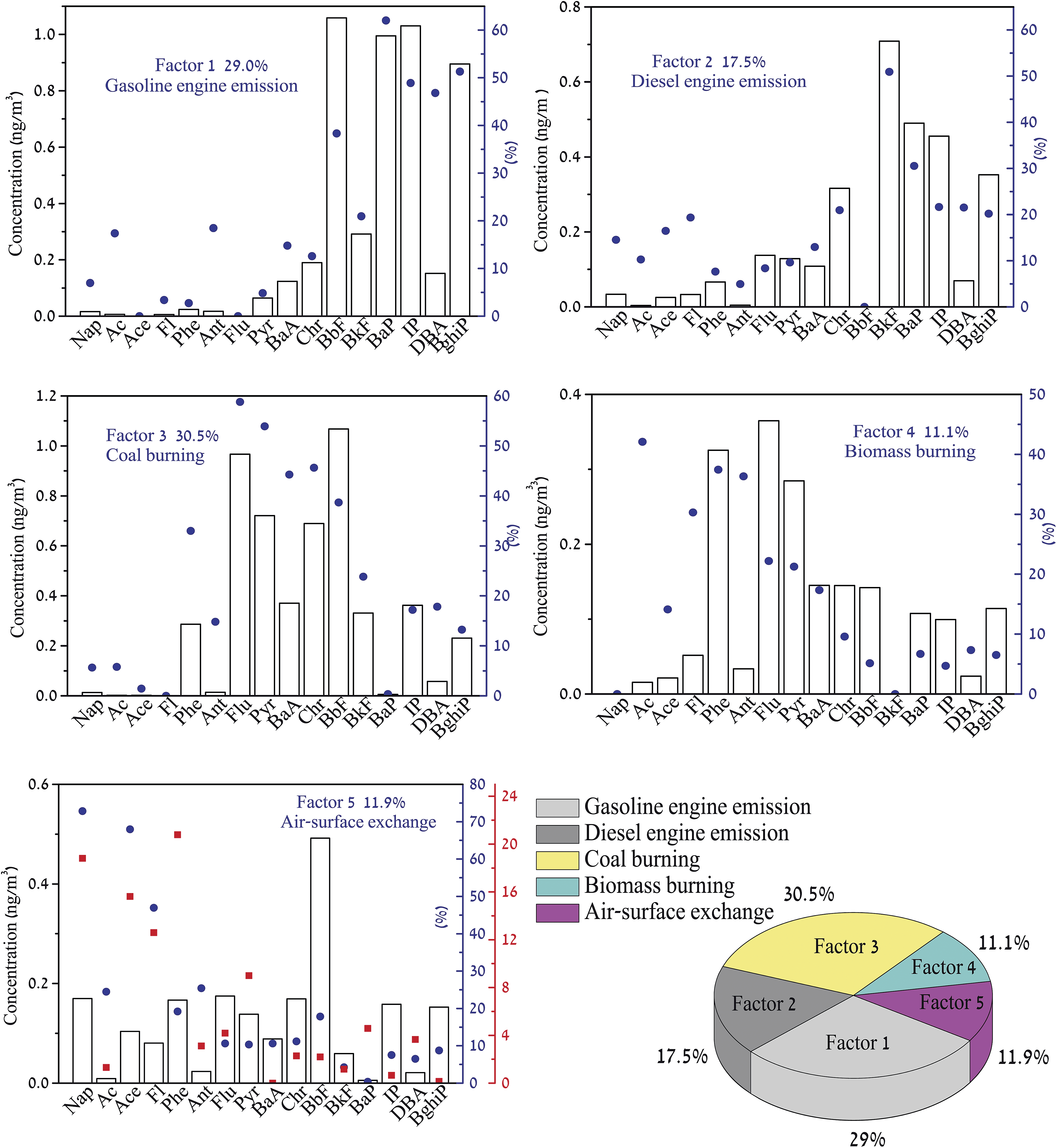

Fig. 4 5-factor loadings by PMF analysis from 16 PAH data of 72 PM2.5 samples collected in Shanghai over four seasons.

Factor 1 accounted for 29.0% of the sum of the measured 16 PAHs. It has a high loading of 5–6 ring PAHs, including BbF, BaP, IP and BghiP, and moderate contributions from BkF, BaA and Chr. This kind of profile is considered to be associated with gasoline engine emission.^31,32 In recent decades, gasoline has been used primarily as a fuel in internal combustion engines of automobiles. As a world megacity, Shanghai has been experiencing a rapid increase in vehicles, especially those for private use. According to ChinaIRN (http://www.chinairn.com/), Shanghai had 1.01 × 10⁶ private vehicles in 2011, a certainly significant use of gasoline by any measure. Therefore, factor 1 is defined as gasoline engine emission sources.

Factor 2 contributed 17.5% of all the measured 16 PAHs. High loadings of BkF, BaP and BghiP and moderate loadings of Flu, Pyr, BaA, and Chr were observed. A similar profile of high loadings of BaP and BghiP was also observed in aerosols in the Hudson River Estuary.³³ By visually comparing with the factor 1, assigned as gasoline engine emission, the profile of factor 2 exhibited more 3–4-ring PAH characteristics. It has been revealed that the diesel emissions are enriched in Flu, Pyr³² and BkF³³ relative to gasoline emissions. Accordingly, factor 2 is characterized as a diesel engine emission source. Diesel fuel has been widely used in trucks and sport utility vehicles (SUVs), since they are more powerful and fuel-efficient than similar-volume gasoline engines.

Factor 3 explained 30.5% of the sum of the measured 16 PAHs. This is dominated by Flu and Pyr, with moderate loadings of BaA, Chr, BbF, and BkF. Flu and Pyr have been considered to be tracers of coal burning.¹ According to NBSC (http://www.stats.gov.cn/english/), coal consumption in China accounted for more than 70% of the total energy used in 2011. As the largest industrial and commercial city in China, Shanghai consumes a large amount of coal. Hence, factor 3 is assigned as coal burning sources.

Factor 4 accounted for 11.1% of all measured 16 PAHs. It was highly loaded with Phe, Ant, Flu, and Pyr, and moderately with BaA, Chr, and BbF. This source profile of PAHs in PM2.5 has been reported in the literature to be mainly from biomass burning.^14,23 In China, including rural areas in the YRD, agricultural refuse, such as straws, stalks, and deadwood, are mostly used for cooking. They are usually burned in primitive stoves without forced blasting, emitting ample organic pollutants, including PAHs.

Factor 5 accounted for 11.9% of all the measured 16 PAHs. This profile contains more volatile PAHs (i.e., 2–3-rings, such as Nap, Ace, Phe) and is readily found in the warm seasons (i.e., fall and summer), as expected for a temperature-driven process. The PAH profiles (% of the factor total) of this factor were similar with those investigated by Wang et al. (2014) (red dot in Fig. 4), which was assigned as an air-surface exchange.¹² In previous studies, Nap has been used as a tracer of the fugitive loss of petroleum products.³⁴ Ace, Fl and Phe are abundant in natural mineral dust transport.²³ Moreover, the low molecular weight (LMW) PAHs are favored in air-surface exchange.³³ Gaseous PAH concentrations have been observed to have an exponential relationship with temperature, due to evaporation from contaminated ground during the warmer weather.³⁵ Dimashki et al. (2001) also recognized this process and suggested that a process of volatilization of these compounds from surfaces might be appreciable for Phe, Fl and Flu.³⁶ In addition, it has been suggested that the soil could also be a potential source of PAHs in the atmosphere, driven by higher temperatures.³⁷ Accordingly, factor 5 could be attributed to air-surface exchange. The “exchange” here indicates a possible re-emission of aged PAHs from “contaminated soil” or volatilization of PAHs directly from the ground into the atmosphere, to be absorbed later by the particles.

The seasonal contributions of each source to the 16 PAHs are shown in Fig. 5. A strong seasonal variation of PAH sources can be seen. Gasoline engine emission and coal burning were the two major sources, both in the fall (36.7% and 27.9, respectively) and in the winter (34.6% and 41.9%, respectively); while diesel engine emission contributed the most in the spring (52.1%) and in the summer (43.5%). In the fall and winter, the prevailing winds in Shanghai are northwesterly. Therefore, aside from the local emission sources, the influence of pollutants transported not only from the YRD but also from northern China on the PAH sources should be taken into account. The intense manufacturing activities of the YRD and northern China demand a large amount of energy, provided mostly by coal-fired power plants, and the large vehicular fleet is a rapidly growing source of emissions. Moreover, the contributions from biomass and coal burning in the winter (57.0%) almost doubled that of the fall (38.3%). Space heating is technically not allowed in the south in winter, while in northern China, centralized heating via coal is provided. For example, in Beijing and Qingdao, the coal and biomass burned in the winter contributed more PAHs in PM2.5 than vehicular emissions,¹⁴ possibly due to the space heating policy in northern China.^17,38 In the spring and summer, the prevailing winds in Shanghai are southeasterly, mostly from the relatively “clean” East China Sea. The prevailing “southeasterly winds” could be further evidenced by the HYSPLIT air mass back trajectory model from the National Oceanic and Atmospheric Administration (http://ready.arl.noaa.gov/hysplit-bin/trajasrc.pl). As a marginal sea off eastern China, the East China Sea has two typical busy ports located adjacent to Shanghai. The Port of Shanghai, the world's busiest container port, set a historic record by handling over 32 million twenty-foot equivalent units (TEUs) in 2012 (http://www.shanghai.gov.cn/). Yangshan Port, a deepwater port for container ships in Hangzhou Bay south of Shanghai, was on track to move 12.3 million TEUs in mid-2011 (http://www.marine-news-china.com). These two ports are used for domestic ferry rides, and also handle cargos for national or international trade. It should be noted that, due to the larger demands of these cargos transported nationwide in China, the number of trucks in Shanghai increased accordingly. In 2011, there were already 3.0 × 10⁴ trucks registered in the Port of Shanghai. Diesel is commonly used instead of gasoline to power the ferry, cargo ships and trucks like this. Considering the wide usage of diesel fuel, as stated above, and the southeasterly winds in the spring and summer off Shanghai, it is reasonable to suggest that the diesel engine emission from maritime activity could be a crucial source of the 16 PAHs in the PM2.5.

Fig. 5 Contributions of the five sources to 16 PAHs in PM2.5 in Shanghai over four seasons.

Conclusions

The annual average concentration of PM2.5-bound 16 PAHs in Shanghai was 16.9 ± 9.0 ng m⁻³. The highest contributor for 16 PAHs was from the 5–6-ring (56.5%), followed by 4-ring (31.1%) and 2–3-ring PAHs (12.4%). Good correlations between the 16 PAHs and organic carbon (OC) were observed in the fall and winter, suggesting their possible common combustion sources; poor correlations were observed in the spring and summer, which could be attributed to the higher SOC formation enhanced by meteorological conditions. PMF identified that gasoline engine emission and coal burning were the two major sources both in the fall and winter (64.6% and 76.5%, respectively); while in the spring and summer, diesel engine emission contributed the most (52.1% and 43.5%, respectively), followed by coal burning (23.9%) and gasoline engine emission (22.5%). These source categories apportioned by PMF could provide valuable information for the possible sources of particle-bound PAHs of megacities in China.

Acknowledgements

This work was supported by the Shanghai Science and Technology Committee (no. 12DJ1400102), and Natural Science Foundation of China (NSFC) (no. 41176085). The anonymous reviewers should be sincerely appreciated for their constructive comments that greatly improved this study.

References

1. R. Harrison, D. Smith and L. Luhana, Environ. Sci. Technol., 1996, 30, 825–832.
2. A. Lima, J. Farrington and C. Reddy, Environ. Forensics, 2005, 6, 109–131.
3. M. Simcik, S. Eisenreich and P. Lioy, Atmos. Environ., 1999, 33, 5071–5079.
4. R. Lohmann, T. Harner, G. Thomas and K. Jones, Environ. Sci. Technol., 2000, 34, 4943–4951.
5. B. Hou, G. Zhuang, R. Zhang, T. Liu and Z. Guo, J. Hazard. Mater., 2011, 190, 529–536.
6. K. Huang, G. Zhuang, Y. Lin, J. Fu and Q. Wang, Atmos. Chem. Phys., 2012, 12, 105–124.
7. J. Feng, C. Chan, M. Fang, M. Hu and L. He, Chemosphere, 2006, 64, 1393–1400.
8. Z. Gu, J. Feng, W. Han, L. Li and M. Wu, J. Environ. Sci., 2010, 22, 389–396.
9. Y. Feng, Y. Chen, H. Guo, G. Zhi and S. Xiong, Atmos. Res., 2009, 92, 434–442.
10. P. Li, X. Li, C. Yang, X. Wang and J. Chen, Atmos. Environ., 2011, 45, 4034–4041.
11. B. Mai, S. Qi, E. Zeng, Q. Yang and G. Zhang, Environ. Sci. Technol., 2003, 37, 4855–4863.
12. F. Wang, T. Lin, Y. Li, T. Ji and C. Ma, Atmos. Environ., 2014, 92, 484–492.
13. J. Chow, J. Watson, L. Pritchett, W. Pierson and C. Frazier, Atmos. Environ., Part A, 1993, 27, 1185–1201.
14. T. Lin, L. Hu, Z. Guo, Y. Qin and Z. Yang, J. Geophys. Res.: Atmos., 2011, 116, D23305.
15. K. He, F. Yang, Y. Ma, Q. Zhang and X. Yao, Atmos. Environ., 2001, 35, 4959–4970.
16. W. Ma, Y. Li, H. Qi, D. Sun and L. Liu, Chemosphere, 2010, 79, 441–447.
17. Z. Guo, L. Sheng, J. Feng and M. Fang, Atmos. Environ., 2003, 37, 1825–1834.
18. J. Li, G. Zhang, X. Li, S. Qi and G. Liu, Sci. Total Environ., 2006, 355, 145–155.
19. J. Zhao, F. Zhang, L. Xu, J. Chen and Y. Xu, Sci. Total Environ., 2011, 409, 5318–5327.
20. M. Minguillón, M. Arhami, J. Schauer and C. Sioutas, Atmos. Environ., 2008, 42, 7317–7328.
21. R. Hamilton, A. Duarte, M. Kendall and T. Rocha-Santos, J. Environ. Monit., 2002, 4, 890–896.
22. J. Dachs, T. Glenn, C. Gigliotti, P. Brunciak and L. Totten, Atmos. Environ., 2002, 36, 2281–2295.
23. K. Moon, J. Han, Y. Ghim and Y. Kim, Environ. Int., 2008, 34, 654–664.
24. J. Dachs and S. Eisenreich, Environ. Sci. Technol., 2000, 34, 3690–3697.
25. Y. Chen, Y. Feng, S. Xiong, D. Liu and G. Wang, Environ. Monit. Assess., 2011, 172, 235–247.
26. J. Cao, S. Lee, K. Ho, S. Zou and K. Fung, Atmos. Environ., 2004, 38, 4447–4456.
27. B. Turpin and J. Huntzicker, Atmos. Environ., 1995, 29, 3527–3544.
28. L. Castro, C. Pio, R. Harrison and D. Smith, Atmos. Environ., 1999, 33, 2771–2781.
29. I. Kavouras, P. Koutrakis, M. Tsapakis, E. Lagoudaki and E. Stephanou, Environ. Sci. Technol., 2001, 35, 2288–2294.
30. M. Yunker, R. Macdonald, R. Vingarzan, R. Mitchell and D. Goyette, Org. Geochem., 2002, 33, 489–515.
31. A. Li, J. Jang and P. Scheff, Environ. Sci. Technol., 2003, 37, 2958–2965.
32. D. Wang, F. Tian, M. Yang, C. Liu and Y. Li, Environ. Pollut., 2009, 157, 1559–1564.
33. J. Lee, C. Gigliotti, J. Offenberg, S. Eisenreich and B. Turpin, Atmos. Environ., 2004, 38, 5971–5981.
34. M. Khairy and R. Lohmann, Chemosphere, 2013, 91, 895–903.
35. K. Gustafson and R. Dickhut, Environ. Sci. Technol., 1997, 31, 3738–3739.
36. M. Dimashki, L. Lim, R. Harrison and S. Harrad, Environ. Sci. Technol., 2001, 35, 2264–2267.
37. T. Agarwal, P. Khillare and V. Shridhar, Environ. Monit. Assess., 2006, 123, 151–166.
38. Z. Guo, T. Lin, G. Zhang, L. Hu and M. Zheng, J. Hazard. Mater., 2009, 170, 888–894.

---

Footnote

† Electronic supplementary information (ESI) available. See DOI: 10.1039/c4em00570h

---