Transition state geometry prediction using molecular group contributions

Abstract

Detailed kinetic models to aid the understanding of complex chemical systems require many thousands of reaction rate coefficients, most of which are estimated, some quite approximately and with unknown uncertainties. This motivates the development of high-throughput methods to determine rate coefficients via transition state theory calculations, which requires the automatic prediction of transition state (TS) geometries. We demonstrate a novel approach to predict TS geometries using a group-additive method. Distances between reactive atoms at the TS are estimated using molecular group values, with the 3D geometry of the TS being constructed by distance geometry. The estimate is then optimized using electronic structure theory and validated using intrinsic reaction coordinate calculations, completing the fully automatic algorithm to locate TS geometries. The methods were tested using a diisopropyl ketone combustion model containing 1393 hydrogen abstraction reactions, of which transition states were found for 907 over two iterations of the algorithm. With sufficient training data, molecular group contributions were shown to successfully predict the reaction center distances of transition states with root-mean-squared errors of only 0.04 Å.

---

Complex chemical systems, such as the combustion of novel renewable fuels, can be better understood with detailed kinetic models. The required detail means a model can contain thousands of species and reactions,¹ making their construction laborious and prone to human error. Automated mechanism generators have been developed to construct detailed kinetic models while avoiding the pitfalls of manual construction.² Thermodynamic and kinetic parameters are preferentially sourced from experimental measurements or high fidelity theoretical calculations to complete a kinetic model, but estimates are also used as many of the required parameters are unknown.³

Parameter estimation methods are computationally efficient strategies to provide thermodynamic and kinetic values.⁴ Most parameter estimation methods are based on Benson's group additivity,⁵ in which the thermodynamics of a molecule are estimated by summing the contributions from the molecular groups present in the molecule, these group values having first been calculated from molecules with known thermodynamic parameters.^6,7 Such group contribution methods have been shown to work well for thermochemistry of hydrocarbon species, and the concept has been extended to kinetic parameter estimation.^8–11 Group contribution methods become less accurate when parameters are estimated using groups values that have not been well determined, due to insufficient training data. For example, group values have been difficult to extend to thermodynamics of fused rings leading to inaccuracies in their estimates.¹²

Such inaccuracies in group-based estimation methods have motivated high-throughput electronic structure calculations for thermodynamics and kinetics.^13,14 Such a procedure was recently developed to calculate thermodynamic parameters within the framework of the automatic Reaction Mechanism Generator (RMG).^12,15,16 In that procedure, 3-dimensional structures were created via distance geometry,¹⁷ with the structures optimized using force-fields and semi-empirical electronic structure calculations to provide molecular parameters, allowing thermodynamic parameters to be calculated. Thermodynamic error was greatly reduced for fused-ring species compared to estimates derived from Benson's group additivity.

In a similar manner, kinetic parameters currently estimated from poorly trained group values could be improved by applying electronic structure calculations and transition state theory, but this requires a high-throughput approach for finding transition state geometries. A transition state geometry estimate, which is typically provided manually, must be quite similar to the correct transition state geometry for the optimization to converge. Manual estimation of transition states is not compatible with the context of automated mechanism generation, which requires thousands or even millions of reaction rates. With continuing advances in computing power, it has become feasible to automate these searches.

One approach used the growing string double-ended method¹⁸ to search for possible transition states.¹⁹ While there is an increased computational cost associated with the transition state search, the use of the string method negates the need for a path analysis step to validate the transition state. This method has been extended to the construction of detailed mechanisms, where the user controls the mechanism generation with restrictions such as barrier height limits.²⁰ Adoption of this method is limited to those with access to software with reliable double-ended methods. Zimmerman has further developed these methods to create a single-ended transition state search.²¹ This makes use of driving coordinates from reactants to find intermediates, from which the transition state can be found using the growing string method.

Zádor and Najm instead use a rule-based approach to direct atoms from a reactant configuration towards the product, using energy calculations at each step to determine the location of the transition state.²² This method is best suited to reaction systems with a small number of atoms, such as the exploration of a pressure dependent reaction network.

The AARON code automates transition state searches to screen potential organocatalysts.²³ A catalyst structure is provided by the user and mapped onto a parent catalyst structure for which the transition state geometry is already known, then a series of partially constrained semiempirical and DFT optimizations allow the new transition state to be found.

Maeda and Morokuma used an artificial force to push reacting molecules together, to probe the potential energy surface around atoms, predicting reactions and finding their transition states.^24,25 This artificial force induced reaction method requires many random starting orientations.

The methods highlighted above explore the potential energy surface for a given set of atoms, finding many reaction pathways for a few reactants. These are not well suited to automated mechanism generation where it is routine to have many reactions of the same type but with varying reactants. For such applications, we propose an alternative method to estimate transition state geometries using molecular group contributions. The group contributions are used to predict inter-atomic distances in the reaction center of the transition states.

Estimated 3D geometries are constructed from the predicted distances using distance geometry. Optimization and validation of the transition state estimates have also been automated. Hydrogen abstraction reactions from a diisopropyl ketone combustion model,²⁶ previously developed using RMG, were used to test the method, with transition states found for over 65% of the 1393 reactions.

Methods

Geometry estimation and optimization

Distance geometry. The open-source cheminformatics toolkit RDKit²⁷ was chosen for its speed and accuracy as a conformer generation tool.²⁸ The distance geometry approach used in RDKit is described by Blaney and Dixon.¹⁷ This approach uses a molecular bounds matrix containing upper and lower bounds on distances separating each atom pair.

Distances separating reactive atoms undergo significant change during a reaction, but the rest of the molecule remains relatively unaffected. As a result, distances between the reactive atoms are unknown at the transition state, but existing methods can be used to determine the remaining distances.

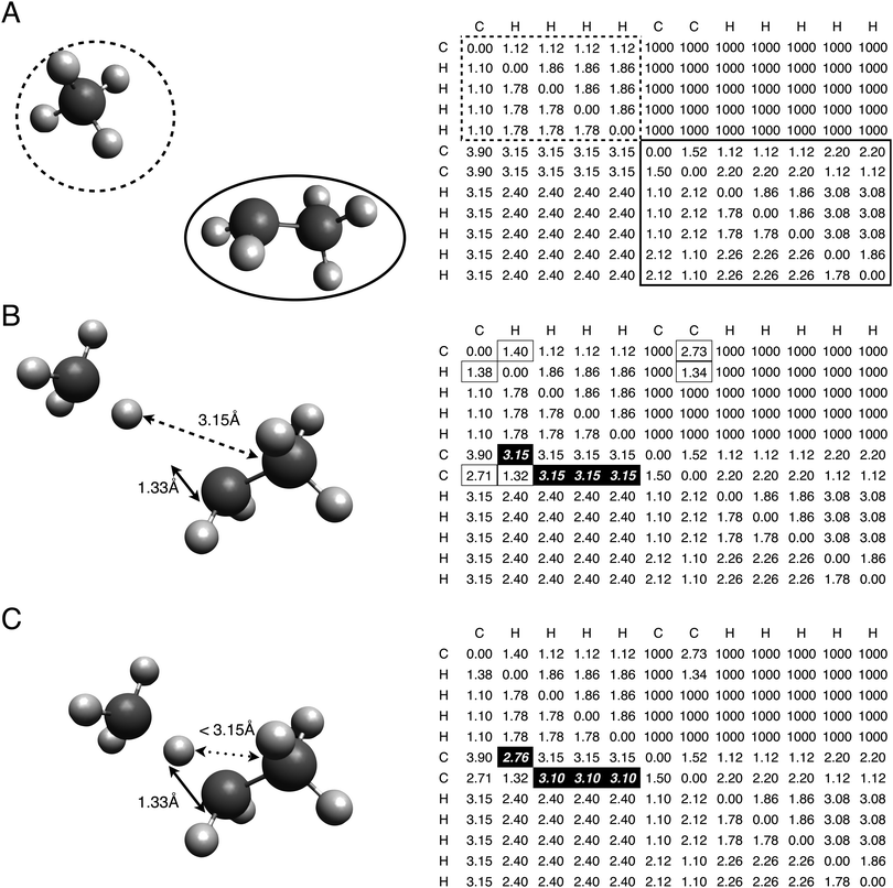
For hydrogen abstraction reactions, three atoms lie in the reaction center: the abstracted hydrogen (H), the atom bonded to the abstracted hydrogen (X), and the radical abstracting the hydrogen (Y). The three distances separating each reactive atom pair are denoted as dXH, dHY, and dXY. Estimating these distances allows the entire transition state geometry to be created using distance geometry. Typically the geometry is specified manually, but we demonstrate here a group contribution method to estimate the required reaction center distances.

Molecular group organization. Molecular groups were used to predict distances separating reactive atoms of transition states. The molecular groups were organized in a hierarchical tree structure, so that distance predictions were made using the most relevant available data. The tree was limited to reactions with only atom types (elements) of C, H, and O, but can be expanded to include other atom types by adding the appropriate groups. Two trees were used as hydrogen abstraction reactions are bimolecular and the reaction center distances are dependent on both reactants. The head nodes (top groups) for the trees were X_H_or_Xanyrad_H and Y_anyrad. The X_H_or_Xanyrad_H tree described the reactant where X is a wildcard atom of any atom type, with zero or more radical electrons, bonded to an H atom (the hydrogen to be abstracted), and the Y_anyrad tree described the abstracting radical of any atom type, with one or more radical electrons. Child nodes were added to be more detailed than the parent nodes, for example, a child of the X_H_or_Xanyrad_H node is X_H (here X is any element but has no radical electrons), itself having a child H2.

The structure of the molecular group tree was first taken from the kinetics database of the RMG software. This tree structure was developed to make efficient use of sparse data for estimating kinetic parameters relevant to hydrocarbon combustion. The development of this tree involved several researchers making independent modifications over a number of years to provide improved kinetic estimates for specific fuels. Sometimes modifications were made with the aim of minimizing disruption of the existing tree, rather than of optimizing the overall tree structure. The uncoordinated nature of the modifications has led to a tree structure that is hierarchical, but lacks obvious logic in its structure, and was certainly not optimized for transition state distances. For example, the O_H group has descendants that are peroxides except for the peroxyradical group (Orad_O_H), which is instead a sibling group.

A new tree structure was also developed for comparison to the RMG designed structure. The new design was built to understand the effect of the tree structure. The same starting head nodes were used for the new tree as they described all possible reacting molecules for the hydrogen abstraction family. Care was taken to ensure subsequent generations had a single characteristic defined across all sibling nodes, and that characteristics thought to be more important were defined earlier (higher in the tree). For example, the children of the head nodes specified the elements of the wildcard atoms (X and Y), but no bonding or radical electrons were specified because, while important, they are less critical than the wildcard atom types. This meant that child nodes to X_H_or_Xanyrad_H were H2, C_H, and O_H (the X is defined as H, C, or O), while the children of Y_anyrad were Hrad, Orad, and Crad. The following two generations defined the radicals and bonding. For the X branch of the tree the bonding was defined first, then the radicals; on the Y branch the radicals were defined first, then the bonding. This convention was continued until the bonding on the nearest neighbor atoms were defined (the R groups in R_X_H and R_Y_rad).

Both the original and the updated trees are available in the ESI.†

Group additive distance estimation. Reaction center distances were collated from previously optimized transition state geometries, creating a training set. Values for molecular groups, organized in a hierarchical tree, were calculated using values from the training set by linear least squares regression, using the distances for every reaction in the training set that match the molecular group. The base value is stored in the top level node, and the value for a descendant is stored as a correction to the top level node value. This means the value of a given node is calculated as the sum of the base value and the node's correction.

The linear least squares regression calculates group values by finding the best fit to the available training data. For each set of distances in the training set, the reactants are matched to groups in the group tree. All groups that match the X_H_or_Xanyrad_H reactant are paired with the groups that match the Y_anyrad reactant, and the sum of each pair and a base value is set equal to the training distances. This creates a system of equations where the variables are the group values and the known values are the training data. The regression is conducted using the linear algebra package in numpy, finding the group values that best fit the data.²⁹ A detailed description of the least squares regression is available in the ESI.†

The reaction CH₄ + C₂H₅ is used as an example. Table 1 shows the sections of the molecular group tree relevant to this reaction. The most specific group that matches each reactant is found by descending the tree. CH₄ matches the C_methane group in the X_H_or_Xanyrad_H tree, while C₂H₅ matches the C_rad/H2/Cs\H3 group in the Y_anyrad tree. An explanation of the naming convention, and complete tree definitions, are provided in the ESI.† The distance estimates are calculated by summing the top node value and the group correction for each reactant, predicting respective values for dXH, dHY, and dXY as 1.388 Å, 1.331 Å, and 2.721 Å.

Table 1 Part of the hierarchical molecular group tree for transition state distances trained using 1071 transition state distances calculated using B3LYP/6-31+G(d,p). The full tree is in the ESI

Group	dXH	dHY	dXY
Base	1.336010	1.336330	2.667560
L1: X_H_or_Xanyrad_H
L2: X_H	−0.002556	0.002864	0.000227
L3: H2	−0.327434	−0.045046	−0.369886
…
L3: Cs_H	0.007461	0.023642	0.032296
L4: C_methane	0.076680	−0.051468	0.028801
L4: C_pri	0.025511	−0.002230	0.025031
L5: etc.
L4: C_sec	−0.026003	0.069757	0.044341
L4: C_ter	−0.025676	0.062321	0.034956
L5: Etc.
L2: Xrad_H	0.094987	−0.106435	−0.008430
Etc.
L1: Y_anyrad
…
L2: Y_rad	0.002857	−0.002500	0.000277
L3: H_rad	−0.044160	−0.330263	−0.371926
…
L3: Cs_rad	0.024200	0.007289	0.032625
L4: C_methyl	−0.050813	0.075919	0.028607
L4: C_pri_rad	−0.001792	0.025273	0.025176
L5: C_rad/H2/Cs	−0.032772	0.051719	0.021617
L6: C_rad/H2/Cs\H3	−0.024753	0.045959	0.024509
L6: C_rad/H2/Cs\Cs2\O	−0.125966	0.025305	−0.097425
Etc.

---

Transition state geometry estimation. With the distances between atoms at the reaction center estimated using molecular group values as described in the previous section, transition state geometry estimates can be created via distance geometry (Fig. 1). For a pair of reactants, a bounds matrix is first generated in RDKit for the stable species, comprising upper and lower limits on the distances between each pair of atoms. For the distances dXH, dXY, and dHY, the values in the bounds matrix are updated to be the distance prediction as described earlier, ±0.05 Å. Some combinations of upper limits from these edits may conflict with previously set lower limits, particularly lower limits between a reactive atom (X, H, or Y) and some non-reacting atoms, forming an inconsistent bounds matrix. In these cases the conflicting lower limits are reduced to be in agreement with the previous edits. Finally, a triangle inequality algorithm is used to smooth the bounds matrix.

Fig. 1 Manipulating the molecular bounds matrix to create transition state geometry estimates. (A) The matrix generated for a pair of stable species. (B) Editing the matrix with the group contribution predictions for transition state distances. (C) Conflicting lower limit distances are corrected, creating a valid transition state distance bounds matrix.

Transition state estimates are created by randomly “embedding” the atoms in 3D space such that they satisfy the bounds matrix. Repeating this process allows multiple conformers to be created. The conformer geometries are then optimized using a UFF force field calculation constrained by the bounds matrix. The lowest energy conformer according to the UFF calculation is selected as the transition state estimate. While the accuracy of the force field energy calculation is low, it is sufficient for conformer selection.

Transition state validation. An algorithm was created to control the transition state refinement and validation. The geometry estimate resulting from the constrained force field optimization, is used as the initial guess for a transition state optimization using electronic structure methods such as density functional theory. The calculation is checked for an absence of errors, and the presence of a single imaginary frequency. The optimized geometry is then used for an intrinsic reaction coordinate (IRC) calculation.³⁰

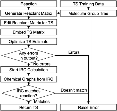
The IRC result should connect the original reactants and products for a successful transition state. The result is typically inspected visually for comparison, but this is not possible for an automatic procedure. In our algorithm, the IRC geometries are extracted and converted into chemical graphs using a simplified version of the connect the dots method in Open Babel.³¹ The atoms are sorted along the z-coordinate, with the method starting with the lowest atom, continuing along the axis, and terminating with the highest. A bond is made between this first atom, A, and its nearest neighbor, B, if all the following are true:

(1) No bond currently exists between A and B

(2) the number of other bonds to A and B is less than their respective valencies

(3) the distance between A and B is less than the sum of their covalent radii +0.2 Å.

The process is repeated with atom A being compared each time to the next-nearest atom from the previous iteration, until either there are no more atoms to be compared or the number of bonds on A equals its valency. The method then proceeds on to the next atom along the z-axis.

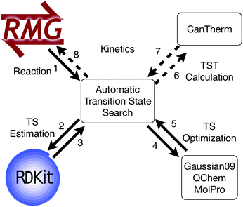
With the bonding complete, the chemical graphs of the IRC molecules are compared to the starting reactants and products using a graph isomorphism algorithm.³² The transition state search is successful if the chemical graphs are isomorphic. The automated algorithm is outlined in Fig. 2.

Fig. 2 The automated transition state search algorithm.

Fig. 3 Distances from 907 validated transition states found at B3LYP/6-31+G(d,p) were compared to predictions derived from molecular group values. The solid line represents parity with the optimized distances, and the dashed lines represent the root mean squared error of the estimates from parity. The predictions improved as the training set used to calculate the group values was expanded.

Training the molecular group values. Molecular group values were trained with known values taken from transition state geometries that were optimized and validated with the B3LYP electronic structure method and a 6-31+G(d,p) basis set. All data added to a training set came from transition states found and validated using the same electronic structure method and basis set. Transition states found and validated with the automated algorithm were also added to the training set at the end of each test of the automated algorithm. Before rerunning the algorithm, the molecular group values were retrained using the training set expanded from the previous run.

Method evaluation

H abstraction reactions from a DIPK combustion model. 1393 hydrogen abstraction reactions from a diisopropyl ketone (DIPK) combustion model (total of 4027 reactions)²⁶ were used to test the automated algorithm. Reactions were passed to the transition state search algorithm, which estimated transition state geometries, then optimized and validated them.

First, a preliminary training set was created from 44 unique hydrogen abstraction transition states, and was used to train the molecular group tree. As few groups were trained, we found the distance estimates to be insufficient for reliably predicting transition states. As a result, the training set was expanded to contain data from a total of 230 transition states. This expansion of the training set was done with geometries found both manually and using the automated algorithm. The reactions from the DIPK model were then passed to the automated algorithm, with data from the successfully found transition states added to the training set. The groups were retrained, and the method was tested again on the same reactions from the DIPK model. This led to the expansion of the training set from data for 230 transition states to 827 and then 1071 transition states. Characteristics of the group contribution method were investigated using 4 training sets (Table 2).

Table 2 Training set information. As the training set was expanded, the RMS error from the validated transition state distances decreases

Training set name	Transition states in training set	Geometries found	RMS error (Å)
			Original tree	Modified tree
44TS	44	Not run	0.181	0.124
230TS	230	658	0.102	0.088
827TS	827	734	0.040	0.042
1071TS	1071	Not run	0.036	0.041

---

Tree structure comparison. The original molecular group tree structure was used to automatically find transition states for hydrogen abstraction reactions in the DIPK combustion model. The new group tree was used to estimate the reaction center distances of the transition states previously found using the original group tree structure. This allowed comparison of the reaction center distance predictions made with either tree for a given training set, without repeating all the electronic structure calculations.

Further comparison tested the performance of the molecular group trees for small training sets. The largest training set (1071TS) was randomly sampled to create many smaller training sets containing data from 44 transition states. With each of the smaller training sets, group values were trained and distances were predicted then compared to known distances from validated transition states. This was done using both the original and new tree structures.

Computational chemistry. Estimated geometries were refined in RDKit using universal force fields (UFF).³³ Geometry optimization and path analysis calculations were run using B3LYP^34,35 with the 6-31+G(d,p)^36,37 basis set in the Gaussian 09³⁸ quantum chemistry package.

Results and discussion

Transition state geometries were successfully estimated using the distance estimates

The algorithm was tested on the DIPK reactions with the groups trained with the training set named ‘230TS’, and found 658 of the 1393 transition state geometries. 597 of the resulting geometries were not already in 230TS, making a set 827TS when added to the training set. The set 827TS was used to retrain the group values, with the algorithm again tested on the DIPK reactions, where 734 transition states were found, of which 244 were unique to the training data. The additional 244 transition states allowed the creation of the 1071TS set. Over the 2 test runs, 907 transition states of the 1393 reactions were found and validated, expanding the training data from 230 to 1071 transition states.

Increasing training data improves the group value predictions. The reaction center distances from the 907 transition states found using the algorithm were compared to distances estimated by molecular group values at differing training set sizes (Fig. 3). The root-mean-squared (RMS) error for each of the 3 distances decreased when the training set containing transition state data was increased from 44 up to 1071 entries. There was little improvement in the estimated values when the training set expanded from 827 geometries to 1071 in comparison to the earlier expansions of the training set.

The observed improvement in the distance predictions as the groups were trained with more data was consistent with our hypothesis. With a larger training set, some untrained groups now have data and some trained groups have more data, improving their accuracy. If the group was newly trained, the algorithm would use more relevant and specific group values, improving the predicted distances. This was observed in the improvement in the distance predictions moving from 44TS to 230TS. With new training data, previously trained groups improve as more data are used to train the group values, as seen when comparing the groups trained using 230TS and 827TS. Little improvement in the RMS error for predictions made with 827TS and 1071TS shows that the 827TS groups were relatively well trained so the extra data from 244 transition state geometries had little effect on group value predictions.

The observations show certain data are more desirable when expanding a training set for molecular group values. For example, if the reactions of interest are hydrogen abstractions from the OH group of an alcohol, the training set should contain such reactions with different types of radicals abstracting the hydrogen. If the training set contains data from a large number of transition states for hydrogen abstractions from alkanes by an alkyl radical, little will be gained by adding a transition state for ethyl abstracting a hydrogen from methane. Both the reactions of interest and the available data should be considered when adding new data to a training set.

Tree structure and data diversity affect prediction accuracy

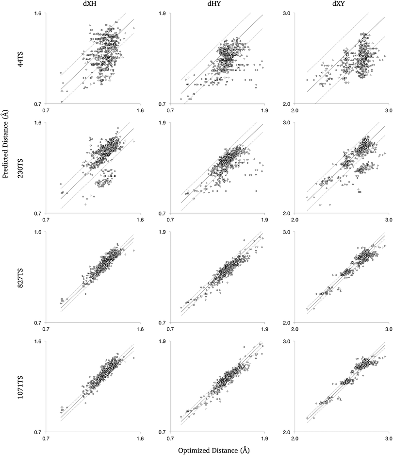
The modified group tree was trained using the same 4 training sets, and distance predictions were made for comparison to the 907 optimized transition states (Fig. 4). Predictions made with the modified structure showed the same trends previously reported: the error decreased as the training sets grew, but the change from 827TS to 1071TS was minimal. The new tree structure produced better estimates than the original for small data sets, where the data is most erroneous. The original tree provides marginally better estimates when trained using large data sets, but the new tree structure is expected to match this accuracy if more detailed groups (more branches in the tree) are added.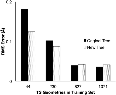

Fig. 4 The RMS error for the distance estimates compared to the optimized transition state distances.

The differences in error observed with the two trees shows the importance of the structure to the distance predictions. While the new tree structure improves the distance predictions from smaller training sets, other tree structures might be able to further improve the predictions.

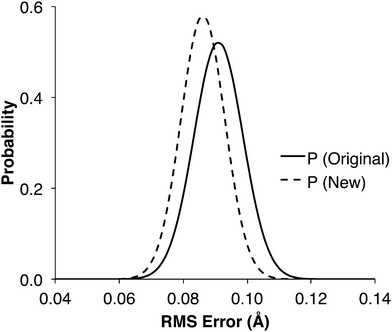
1000 new training sets containing data from 44 transition states were created by randomly selecting data from the 1071TS training set. The new training sets were used to train both the original and new molecular group trees, and reaction center distances were predicted for comparison with the 907 known TS. In over 85% of the 1000 cases, the modified tree had a lower RMS error than the original tree. The probability distribution of the RMS errors (Fig. 5) show that the predictions should be more accurate if made using the modified tree instead of the original tree structure, given the small size of the training set.

Fig. 5 Probability distribution for the root-mean-squared error of the reaction center distances when training the groups with a randomly chosen set of 44 transition state distances, for the original and new tree structures.

The RMS error attained using the 44TS training set was 0.181 Å with the original tree and 0.124 Å with the modified tree (Table 2). Comparing with the probability distributions in Fig. 5, which peak around 0.09 Å, shows that the probability of randomly selecting from 1071TS the 44 transition states used in 44TS is very low, i.e. they are strongly correlated and non-random. This lack of variety in the 44TS set is what leads to the large RMS errors: some specific groups were well trained, but the overall tree was poorly trained. This shows that the value of each transition state in a training set decreases when a similar transition state already exists in that training set, i.e. it is important to have a variety of structures in the training data, distributed evenly across the tree.

Geometry estimation needs improvement to make best use of predicted values

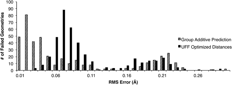
As described earlier, two attempts were made to find all the transition states in the DIPK model: first with the original group tree trained with the 230TS training set, and secondly trained with the 827TS training set. Of the 907 geometries found over these two iterations, 422 were found during one iteration but not the other. This allowed comparison of estimates that were unsuccessful, against the true optimized values from the successful attempts (Fig. 6). One cluster of failures, with RMS errors greater than 0.15 Å, came from the 230TS iteration, and were mostly successful at the 827TS iteration. For distance estimates with RMS errors below 0.05 Å, the conversion from a predicted value into a UFF-optimized 3D geometry using the current algorithm resulted in additional error being introduced into the distances, possibly causing the failure. This suggests that while the group additive method can make accurate distance predictions, further optimization of the algorithm for converting these distances into 3D geometries is necessary.

Fig. 6 422 transition states found in one trial of the algorithm were unsuccessful in another. Comparing optimized distances against the failed estimation attempt showed: (1) poorly estimated distances that were improved when the training set was expanded (2) the conversion from prediction to geometry estimate introduced additional error.

Fig. 7 shows the probability of a failed transition state search increases with increasing root mean squared (RMS) error in the three reacting distances of the starting geometry. The lower bound probabilities are calculated from trials from the 230TS training set. It is a lower bound of P(failure) because only the 249 failures that later succeeded with the 827TS training set were included; for the 486 reactions that continued to fail, the true distances are not known and the RMS error could not be calculated. Because few of our starting geometries were worse than 0.2 Å we do not have many trials in this region and our estimate of the failure probability is quite uncertain, hence the wide Clopper–Pearson³⁹ 95% confidence interval of P(failure) (the vertical bars in Fig. 7). To estimate the upper bound of the failure probabilities, we distributed the 486 additional failures using a variety of assumptions, each giving a different estimate of the P(failure) curve; the upper bound in the figure encompasses all these curves.

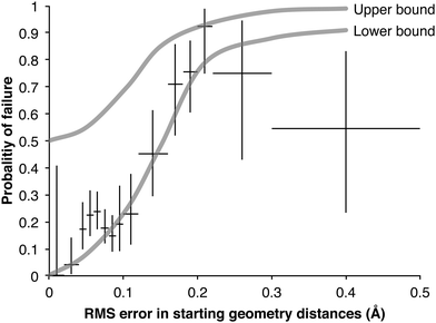Fig. 7 Probability of a failed TS search as a function of RMS error in reactive distances of starting geometry. For each point the vertical bar show the Clopper–Pearson³⁹ 95% confidence interval of the lower bound and the horizontal bar shows the range of RMS errors used to calculate it.

Although uncertain, the shapes of these bounds are informative, and they support the need for good starting geometries for a transition state search: embedded geometries with an RMS error greater than 0.15 Å have a high failure rate. Other reaction families, optimization algorithms, and software packages may behave differently.

Algorithm optimization. The automated algorithm takes advantage of the molecular group estimates to predict, optimize, and validate transition state geometries, but it does not make best use of the group-based distance estimates, and could be improved in future work. In the algorithm tested here, after the atoms are positioned in the 3D space, a constrained UFF refinement step is done in RDKit before the transition state search at DFT. This is designed to improve the geometry of the non-reacting atoms, but the refinement can alter the reaction center distances, dragging them away from their well-predicted values. This could be addressed by tightening the constraint spring constants before the UFF refinement or replacing the refinement step with a DFT optimization with the reaction center distances frozen as is done in the AARON code.²³

The difference between the upper and lower bounds for the reaction center distance estimates is currently set to 0.1 Å, which can be as much as 10% of some distances. This range should be related to the uncertainty calculated when determining the group values by linear regression, allowing well known values to have tight restrictions.

Other reaction families and TST calculations. The algorithm has been tested on hydrogen abstraction reactions, but can be easily extended to other reaction families as long as the reaction is not barrierless. A group tree and an initial training set need to be created for each reaction family, but the algorithm can be used with little modification. Other reaction families may require different levels of precision for eigenvector-following optimization algorithms to succeed, depending on the nature of the Hessian in the vicinity of the transition state.

Transition state searches facilitate kinetic calculations, but automating the entire kinetic calculations would also require the reactant and product geometries. These can be found using the existing automated thermodynamic parameter calculation algorithm.¹² With the required geometries and calculations, the procedure could interface with thermodynamic and kinetic parameter calculators, such as CanTherm (Fig. 8).⁴⁰

Fig. 8 Proposed workflow to complete the automation of kinetic calculations. The solid arrows represent the progress reported in this manuscript, while the dashed arrows represent future work to calculate kinetic parameters via transition state theory.

Conclusion

Automated transition state searches have previously been described as an important challenge for studying complex chemical systems, helping to move mechanism generation closer to being predictive. A group contribution method has been developed to take advantage of available chemical data to make predictions of transition state geometries. The group contribution method performs best with well trained groups, but evidence suggests it can perform reasonably with sparse data if the group tree design is thoughtfully considered. Aside from tree design, predictions can be improved by adding more training data, and the value of the new data increases the more unique it is in relation to the existing training data. The group contributions were used in a novel, fully automated algorithm to create a transition state estimate using distance geometry methods, with the estimate then optimized and validated to find the true transition state structure. The validation step makes it a self-improving machine learning algorithm, as new transition state data are used to improve group values. That a simple sum of contributions from the abstracting and donating groups can so fully determine the transition state geometry offers new physical insight into these reactions. Although the algorithm for generating 3D geometries from distances is a first generation and could be improved, the simple method for predicting the interatomic distances is already remarkably accurate with typical root-mean-squared errors of 0.04 Å.

Acknowledgements

The authors thank the developers of RMG at both Northeastern University and the Massachusetts Institute of Technology for helpful discussions, and Jason Cain for help finding some transition state geometries. Acknowledgment is made to the Donors of the American Chemical Society Petroleum Research Fund for partial support of this research.

References

1. T. Lu and C. K. Law, Prog. Energy Combust. Sci., 2009, 35, 192–215.
2. E. S. Blurock, F. Battin-Leclerc, T. Faravelli and W. H. Green, Cleaner Combustion, Springer London, London, 2013, pp. 59–92.
3. L. J. Broadbelt and J. Pfaendtner, AIChE J., 2005, 51, 2112–2121.
4. J. Yu, R. Sumathi and W. H. Green, J. Am. Chem. Soc., 2004, 126, 12685–12700.
5. S. W. Benson, Thermochemical kinetics: methods for the estimation of thermochemical data and rate parameters, Wiley, New York, 2nd edn, 1976.
6. R. Sumathi and W. H. Green, J. Phys. Chem. A, 2002, 106, 7937–7949.
7. N. Sebbar, H. Bockhorn and J. W. Bozzelli, Phys. Chem. Chem. Phys., 2003, 5, 300–307.
8. M. Saeys, M.-F. Reyniers, G. B. Marin, V. Van Speybroeck and M. Waroquier, J. Phys. Chem. A, 2003, 107, 9147–9159.
9. M. Saeys, M.-F. Reyniers, G. B. Marin, V. Van Speybroeck and M. Waroquier, AIChE J., 2004, 50, 426–444.
10. M. Saeys, M.-F. Reyniers, V. Van Speybroeck, M. Waroquier and G. B. Marin, ChemPhysChem, 2006, 7, 188–199.
11. A. G. Vandeputte, M. K. Sabbe, M.-F. Reyniers and G. B. Marin, Phys. Chem. Chem. Phys., 2012, 14, 12773–12793.
12. G. R. Magoon and W. H. Green, Comput. Chem. Eng., 2012, 52, 35–45.
13. A. McIlroy, G. McRae, V. Sick, D. L. Siebers, C. K. Westbrook, P. J. Smith, C. A. Taatjes, A. Trouve, A. F. Wagner, E. Rohlfing, D. Manley, F. Tully, R. Hilderbrandt, W. H. Green, D. Marceau, J. O'Neal, M. Lyday, F. Cebulski, T. R. Garcia and D. Strong, Basic Research Needs for Clean and Efficient Combustion of 21st Century Transportation Fuels, USDOE Office of Science (SC) (United States) technical report, 2006.
14. C. K. Law, E. A. Carter, J. H. Chen, F. L. Dryer, F. N. Egolfopoulos, W. H. Green, N. Hansen, R. K. Hanson, Y. Ju, S. J. Klippenstein, S. B. Pope, C. J. Sung, D. G. Truhlar and H. Wang, First Annual Conference of the Combustion Energy Frontier Reseach Center (CEFRC), 2010.
15. C. Gao, J. W. Allen, W. H. Green and R. H. West, Comput. Phys. Commun., 2015 , submitted.
16. RMG – Reaction Mechanism Generator, open-source software, http://rmg.mit.edu.
17. J. M. Blaney and J. S. Dixon, Reviews in Computational Chemistry, John Wiley & Sons, Inc., Hoboken, NJ, USA, 1994, vol. 5, ch. 6, pp. 299–335.
18. B. Peters, A. Heyden, A. T. Bell and A. Chakraborty, J. Chem. Phys., 2004, 120, 7877–7886.
19. P. M. Zimmerman, J. Comput. Chem., 2013, 34, 1385–1392.
20. P. M. Zimmerman, Mol. Simul., 2014, 41, 43–54.
21. P. M. Zimmerman, J. Comput. Chem., 2015, 36, 601–611.
22. J. Zádor and H. N. Najm, KinBot: An Automated Code for Exploring Reaction Pathways in the Gas Phase, Sandia National Laboratories Technical Report SAND2012-8095, 2012.
23. B. J. Rooks, M. R. Haas, D. Sepúlveda, T. Lu and S. E. Wheeler, ACS Catal., 2014, 5, 272–280.
24. S. Maeda and K. Morokuma, J. Chem. Theory Comput., 2011, 7, 2335–2345.
25. S. Maeda, T. Taketsugu and K. Morokuma, J. Comput. Chem., 2014, 35, 166–173.
26. J. W. Allen, A. M. Scheer, C. W. Gao, S. S. Merchant, S. S. Vasu, O. Welz, J. D. Savee, D. L. Osborn, C. Lee, S. Vranckx, Z. Wang, F. Qi, R. X. Fernandes, W. H. Green, M. Z. Hadi and C. A. Taatjes, Combust. Flame, 2014, 161, 711–724.
27. G. Landrum, RDKit: Open-source cheminformatics, http://www.rdkit.org.
28. J.-P. Ebejer, G. M. Morris and C. M. Deane, J. Chem. Inf. Model., 2012, 52, 1146–1158.
29. S. van der Walt, S. C. Colbert and G. Varoquaux, Comput. Sci. Eng., 2011, 13, 22–30.
30. K. Fukui, Acc. Chem. Res., 1981, 14, 363–368.
31. N. M. O'Boyle, M. Banck, C. A. James, C. Morley, T. Vandermeersch and G. R. Hutchison, J. Cheminf., 2011, 3, 33.
32. L. P. Cordella, P. Foggia, C. Sansone and M. Vento, IEEE Trans. Pattern Anal. Mach. Intell., 2004, 26, 1367–1372.
33. A. K. Rappe, C. J. Casewit, K. S. Colwell, W. A. Goddard and W. M. Skiff, J. Am. Chem. Soc., 1992, 114, 10024–10035.
34. A. D. Becke, J. Chem. Phys., 1993, 98, 5648–5652.
35. P. J. Stephens, F. J. Devlin, C. F. Chabalowski and M. J. Frisch, J. Phys. Chem., 1994, 98, 11623–11627.
36. T. Clark, J. Chandrasekhar, G. n. W. Spitznagel and P. V. R. Schleyer, J. Comput. Chem., 1983, 4, 294–301.
37. V. A. Rassolov, M. A. Ratner, J. A. Pople, P. C. Redfern and L. A. Curtiss, J. Comput. Chem., 2001, 22, 976–984.
38. M. J. Frisch, G. W. Trucks, H. B. Schlegel, G. E. Scuseria, M. A. Robb, J. R. Cheeseman, G. Scalmani, V. Barone, B. Mennucci, G. A. Petersson, H. Nakatsuji, M. Caricato, X. Li, H. P. Hratchian, A. F. Izmaylov, J. Bloino, G. Zheng, J. L. Sonnenberg, M. Hada, M. Ehara, K. Toyota, R. Fukuda, J. Hasegawa, M. Ishida, T. Nakajima, Y. Honda, O. Kitao, H. Nakai, T. Vreven, Jr, J. A. Montgomery, Jr, J. E. Peralta, F. Ogliaro, M. Bearpark, J. J. Heyd, E. Brothers, K. N. Kudin, V. N. Staroverov, R. Kobayashi, J. Normand, K. Raghavachari, A. Rendell, J. C. Burant, S. S. Iyengar, J. Tomasi, M. Cossi, N. Rega, J. M. Millam, M. Klene, J. E. Knox, J. B. Cross, V. Bakken, C. Adamo, J. Jaramillo, R. Gomperts, R. E. Stratmann, O. Yazyev, A. J. Austin, R. Cammi, C. Pomelli, J. W. Ochterski, R. L. Martin, K. Morokuma, V. G. Zakrzewski, G. A. Voth, P. Salvador, J. J. Dannenberg, S. Dapprich, A. D. Daniels, Ö. Farkas, J. B. Foresman, J. V. Ortiz, J. Cioslowski and D. J. Fox, Gaussian 09, Gaussian, Inc., Wallingford, CT, 2009.
39. C. J. Clopper and E. S. Pearson, Biometrika, 1934, 26, 404.
40. S. Sharma, M. R. Harper and W. H. Green, CanTherm: Open-source software for thermodynamics and kinetics, 2010.

---

Footnote

† Electronic supplementary information (ESI) available: Tables of group values, list of test reactions, and 3-D geometries of transition states. See DOI: 10.1039/c5cp04706d

---