The effect of external heat transfer on thermal explosion in a spherical vessel with natural convection
Received
20th April 2015
, Accepted 1st June 2015
First published on 1st June 2015
Abstract
When any exothermic reaction proceeds in an unstirred vessel, natural convection may develop. This flow can significantly alter the heat transfer from the reacting fluid to the environment and hence alter the balance between heat generation and heat loss, which determines whether or not the system will explode. Previous studies of the effects of natural convection on thermal explosion have considered reactors where the temperature of the wall of the reactor is held constant. This implies that there is infinitely fast heat transfer between the wall of the vessel and the surrounding environment. In reality, there will be heat transfer resistances associated with conduction through the wall of the reactor and from the wall to the environment. The existence of these additional heat transfer resistances may alter the rate of heat transfer from the hot region of the reactor to the environment and hence the stability of the reaction. This work presents an initial numerical study of thermal explosion in a spherical reactor under the influence of natural convection and external heat transfer, which neglects the effects of consumption of reactant. Simulations were performed to examine the changing behaviour of the system as the intensity of convection and the importance of external heat transfer were varied. It was shown that the temporal development of the maximum temperature in the reactor was qualitatively similar as the Rayleigh and Biot numbers were varied. Importantly, the maximum temperature in a stable system was shown to vary with Biot number. This has important consequences for the definitions used for thermal explosion in systems with significant reactant consumption. Additionally, regions of parameter space where explosions occurred were identified. It was shown that reducing the Biot number increases the likelihood of explosion and reduces the stabilising effect of natural convection. Finally, the results of the simulations were shown to compare favourably with analytical predictions in the classical limits of Semenov and Frank-Kamenetskii.
1. Introduction
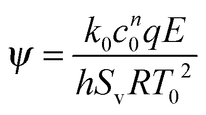
When any exothermic reaction occurs in a closed vessel then there is a risk of thermal explosion. Such explosions occur when the rate of heat production by the reaction exceeds the rate of heat removal through the vessel's walls. The pioneering works on thermal explosion by Semenov1 and Frank-Kamenetskii2 considered two extreme cases. Semenov investigated cases where the mixing within the vessel was so efficient that its contents could be considered to be spatially uniform. He proposed a dimensionless group, which has come to be known as the Semenov number,| |  | (1) |
Semenov showed that an explosion would occur when ψ exceeds the critical value of 1/e. In contrast, Frank-Kamenetskii considered a case without mixing. In such a scenario, spatial temperature gradients develop. Frank-Kamenetskii realised that these gradients would significantly impact the heat removal from the system, and hence the tendency to explode. In particular, he considered cases where heat transfer occurred by conduction only. Frank-Kamenetskii defined the parameter δ = L2k0cn0qE/κρ0CPRT02 and showed that explosion occurred when δ exceeded a critical value, which was dependent on the geometry.
If the temperature gradients become sufficiently large, the resulting buoyancy forces will cause the gas to move. This natural convection can have a significant influence on the progress of the reaction. The nature of the induced flow is determined by the Rayleigh number, Ra = (βgL3ΔT)/(κν). Frank-Kamenetskii2 suggested that in a gaseous system, natural convection becomes significant when Ra > 104; however, further studies3–5 have shown that natural convection becomes important when Ra exceeds ∼500.
The initial experimental evidence3 for a greater influence of natural convection than was allowed for by Frank-Kamenetskii in his model inspired a number of experimental and numerical investigations of exothermic reactions with natural convection. The experimental work of Merzhanov and Shtessel6 on liquid systems in a horizontal cylinder showed that natural convection is significant at Rayleigh numbers well below 104. These empirical observations of the effects of natural convection at lower values of Ra are supported by the analytical and numerical work of Jones7 and Shtessel et al.;8 they showed that when a zeroth-order reaction (i.e. one in which the depletion of the reactant is ignored) occurs between parallel plates, the critical Rayleigh number for the onset of convection is again ∼500. Jones7 also noted that inside a horizontal cylinder or a sphere, there is always some convection, because of the existence of temperature gradients perpendicular to the gravity vector; the ‘onset’ of convection is in fact merely the point where the effects of this flow become observable. In a seminal work on the interaction of thermal explosion and natural convection, Merzhanov and Shtessel9 presented a detailed numerical and experimental analysis of explosion in a liquid system. They showed that natural convection suppresses explosion, and that when explosion does occur, the ignition delay is longer in the presence of natural convection.
In all of these numerical studies, the effect of Ra on thermal explosion was quantified by calculating a new critical value of the Frank-Kamenetskii number, δ. More recently, a new approach was proposed by Liu et al.,10 who presented an analysis in which the explosive limits were described in terms of a series of ratios of characteristic timescales for the important physical processes that are at work, namely natural convection, diffusion (of both heat and mass) and heating due to the chemical reaction. This approach is very attractive, as it describes the transition to explosion in terms of simple groups, which have clear physical meaning. Liu et al.10 summarised their results using a new regime diagram, where the ordinate is the ratio of the timescales for heating and diffusion and the abscissa is the ratio of the timescales for heating and convection. Liu et al.10 also presented clear criteria whereby the effect of consumption of reactant on the progress of an explosion could be ignored. Thus, they identified regions of parameter space when explosions occurred without10 and subsequently with11 reactant consumption included. Significantly, Liu et al.11 also revisited the issue of defining when an explosion can be deemed to have occurred in a system with significant depletion of reactant. This transition to explosion is obvious in systems with minimal reactant consumption, where in an explosive case the temperature will increase without bound; however, when the reactant is depleted, this will significantly reduce the production of heat by the reaction. Consequently, a plot of the temporal development of the maximum temperature in the vessel will display a clear maximum. Liu et al.11 proposed a simple criterion to determine whether an explosion has occurred based solely on the maximum dimensionless temperature achieved. When this exceeds 5, an explosion is said to have occurred. This simple criterion was also shown to be applicable in cases with more complex chemical reactions occuring,12,13 and in reactors where both natural and forced convection are important.14,15
Many other numerical studies have considered the effect of natural convection on explosion in so-called class A geometries (i.e. parallel plates, infinite cylinders and spheres). A comprehensive listing can be found elsewhere.10 These studies, however, all consider cases in which the fixed boundaries of the reactor are held at a constant temperature. This constant temperature at the wall implies there is an infinite heat transfer coefficient between the reactor and its surroundings. In reality, this is unlikely to be the case. There will, of course, be a heat transfer resistance associated with conduction through the solid wall of the reactor, and a finite resistance between the wall and the environment. It is obvious that these additional heat transfer mechanisms may significantly alter the rate of heat removal from the reactor, and hence the tendency of the fluid to explode. Despite this important fact, very few studies have included the effect of external heat transfer in their analyses. Frank-Kamenetskii2 did derive an approximate expression for the dependence of δ in a purely diffusive system on external heat transfer, via what he called a Nusselt number, but what is in reality a Biot number. He found that the inclusion of external heat transfer made an explosion more likely. Boddington et al.16 performed an elegant asymptotic analysis of a purely diffusive system in which consumption of reactant is important. They showed that external heat transfer, again characterised by a Biot number, had a more significant effect in a spherical system, when compared with the other class A geometries.
This work aims to perform an initial investigation into the transition from a slow reaction to explosion in a spherical reactor in which natural convection is significant. As will be justified below, the depletion of the reactant will be ignored. The governing equations are presented in Section 2. The results of numerical simulations are discussed in Section 4. In addition, the results are compared with the analytical results of Semenov and Frank-Kamenetskii.
2. Theoretical background
2.1 Dimensional equations
The reaction occurring in a spherical reactor is considered to be of the formi.e. it is considered to be an nth order exothermic, thermal decomposition reaction. The governing equations express the conservation of the reactant, energy, momentum and mass. The Boussinesq approximation, in which density changes are ignored in all terms except the body forces (which drive natural convection) in the Navier–Stokes equations, is applied to considerably simplify the equations. The Boussinesq approximation requires that the characteristic temperature rise ΔT is such that ΔT ≪ T0; otherwise, full compressibility needs to be taken into account. This approximation is commonly used in the analysis of buoyant flows.17 This approach has been used extensively in the study of thermal explosion,6–15,18–20 as well as other exothermic reactions,21–28 under the influence of natural convection.
The equation governing the conservation of the reactant can be written as:
| | 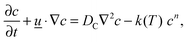 | (3) |
where
c is the concentration of the reactant,
![[u with combining low line]](https://www.rsc.org/images/entities/i_char_0075_0332.gif)
is the velocity vector,
DC is the molecular diffusivity and
n is the order of the reaction. The rate constant
k is assumed to have Arrhenius temperature dependence,
i.e. it has the form
k =
Z![[thin space (1/6-em)]](https://www.rsc.org/images/entities/char_2009.gif)
exp(−
E/
RT), where
Z is the pre-exponential factor and
E is the activation energy. It should be noted that the diffusion is assumed to be Fickian,
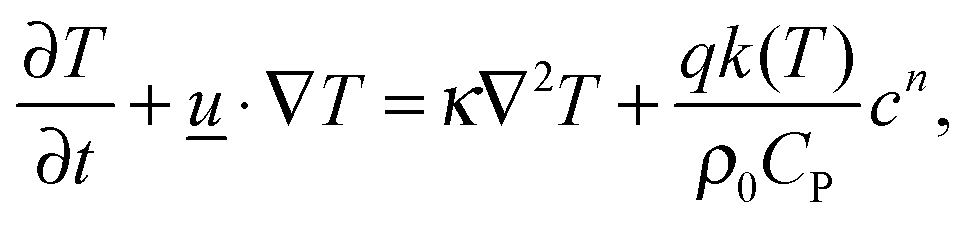
i.e. the diffusive flux is proportional to concentration gradients, as opposed to gradients in mole fraction. This is a consequence of the adoption of the Boussinesq approximation. The conservation of energy within the reactor is described by:
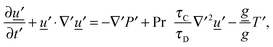
| | 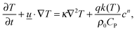 | (4) |
where
CP is the mixture's specific heat at constant pressure,
T is its temperature,
κ is the thermal diffusivity,
ρ0 is the density at the initial temperature
T0 and
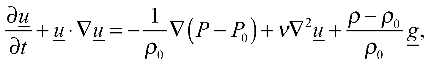
q is the exothermicity of the reaction. The familiar Navier–Stokes equations:
| | 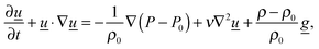 | (5) |
describe conservation of momentum, where
P is the pressure in the reactor and
ν is the kinematic viscosity. Per the Boussinesq approximation, the density only varies in the buoyancy term of
eqn (5), in which
ρ =
ρ0[1 −
β(
T −
T0)], where
β is the coefficient of thermal expansion.
The final equation required is the continuity equation. Adoption of the Boussinesq approximation allows the continuity equation to be written in its incompressible form, i.e.
| | | ∇· = 0 | (6) |
Initially, the reactor is considered to contain the reactant at a concentration
c0, and the contents are assumed to be well-mixed. The gas is also assumed to be initially motionless and at a uniform temperature
T0; this is the temperature of the surrounding environment, which remains fixed throughout the course of the reaction. The external resistance to heat transfer is modelled
via a heat transfer coefficient. This condition, of course, means that the temperature of the wall will not remain constant over the duration of the simulation. It is assumed that the no-slip condition applies at the wall and that there is no flux of any species at the wall. The effects of any heterogeneous reactions at the wall have hence been ignored. The initial and boundary conditions can thus be stated:
t = 0: c = c0; T = T0; = 0 ∀![[x with combining low line]](https://www.rsc.org/images/entities/i_char_0078_0332.gif) |
| | At the wall: ![[n with combining low line]](https://www.rsc.org/images/entities/i_char_006e_0332.gif) ·∇c = = 0; ·(−kT∇T) = h(T − T0), ·∇c = = 0; ·(−kT∇T) = h(T − T0), | (7) |
where
is a unit vector perpendicular to the wall of the vessel.
2.2 Dimensionless equations
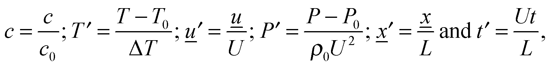
Following the method proposed by Liu et al.10 the governing eqn (3)–(7) can be made dimensionless by the introduction of the following dimensionless variables:| | 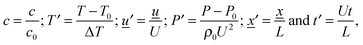 | (8) |
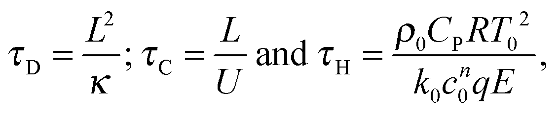
where ΔT = RT02/E is a characteristic scale for the rise in temperature due to the reaction, U = (βgLΔT)1/2 is a characteristic velocity when natural convection dominates transport and L is the characteristic length scale for the reactor, taken to be the radius in the present work. Additionally, the following characteristic timescales can be defined:| |  | (9) |
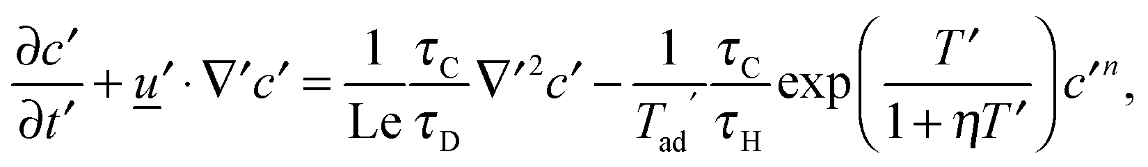
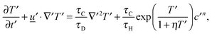
for diffusion, natural convection and heating due to the reaction, respectively. Here, k0 is the rate constant evaluated at the initial temperature T0. Eqn (8) and (9) allow the governing eqn (3)–(7) to be written as dimensionless form as:| | 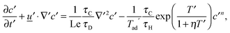 | (10) |
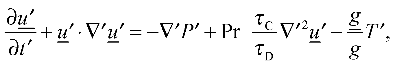
| |  | (11) |
| |  | (12) |
| | | ∇′·′ = 0, | (13) |
| t′ = 0: c′ = 1; T′ = 0; ′ = 0 ∀′ |
| | | At the wall: ·∇′c′ = ′ = 0; −·∇′T′ = BiT′, | (14) |
where Le = κ/DC is the Lewis number, Tad′ = qc0E/(ρ0CPRT02), η = RT0/E, Pr = ν/κ is the Prandtl number and Bi = hL/kT is the Biot number. It should be noted that the form of Bi is slightly different to the classical definition, which uses the ratio of volume and surface area as the characteristic length scale.29 For a spherical reactor this length is L/3, hence the form in eqn (14) only differs from the classical definition by a factor of 3. The limiting cases of constant wall temperature and perfect mixing are represented by Bi = ∞ and Bi = 0, respectively. The governing dimensionless eqn (10)–(13) are the same as those presented previously,10 whilst the boundary conditions in eqn (14) differ.
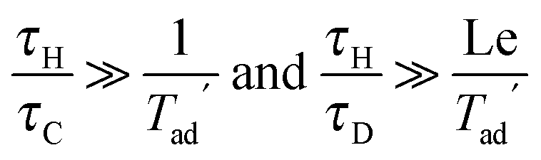
The following criteria were proposed,10 based on the equations above, to determine whether the consumption of reactant is significant. Specifically, if
| | 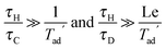 | (15) |
then it may be assumed that the concentration of the reactant is approximately constant throughout the course of the reaction and
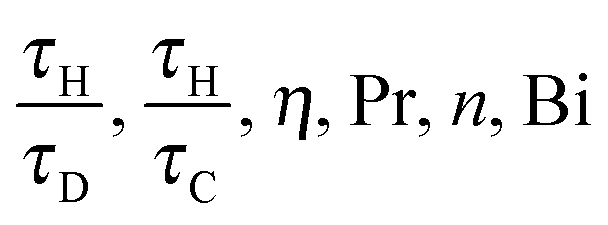
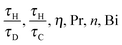
eqn (10) can be ignored. For the purposes of this initial study, this is assumed to be the case. Thus, only the equations for the conservation of energy, momentum and mass must be solved. The behaviour of this system can therefore be characterised by the following six dimensionless groups:
| |  | (16) |
and for a given chemical system, where
η, Pr and
n are fixed, then the behaviour of the system is governed by the ratios
τH/
τD and
τH/
τC, as well as Bi. For a system with a constant wall temperature, the behaviour is only a function of the ratios of timescales as Bi would be infinite. This led to the proposal
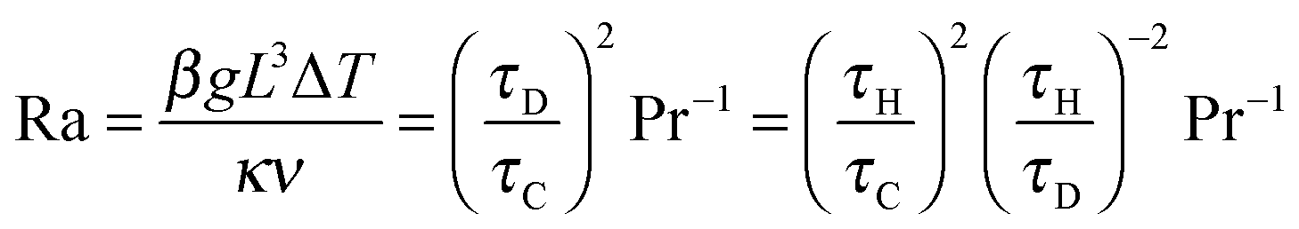
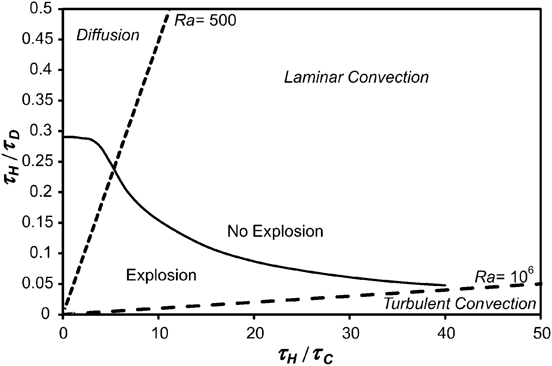
10 of the regime diagram, such as shown in
Fig. 1, to describe the system. The vertical axis represents the purely conductive limit,
i.e. that considered by Frank-Kamenetskii. Lines of constant Ra can be drawn by recognising that
| | 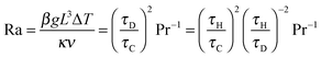 | (17) |
and hence straight lines through the origin in
Fig. 1 will have constant Ra. Shown in
Fig. 1 are lines for Ra = 500 and 10
6. For Ra < 500 diffusion is the dominant transport mechanism, for 500 < Ra < 10
6 laminar natural convection is present and for Ra > 10
6 the convection is turbulent.
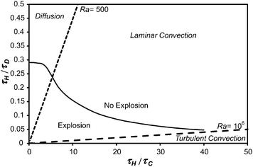 |
| | Fig. 1 The explosion diagram proposed by Liu et al.10 Plotted on the ordinate is the ratio of the characteristic timescales for heating by the reaction and the diffusion of heat and on the abscissa, the ratio of the timescales for heating and convection. The dashed lines represent constant values of Ra (500 and 106) and separate the parameter space into regions where diffusion, laminar natural convection and turbulent natural convection dominate the transport of heat and mass. The solid black line represents the boundary between the stable and explosive regions for Bi = ∞ (i.e. when the temperature of the wall remains constant) in a spherical vessel. The explosive boundary was found by performing many simulations and agrees with that found previously.10 | |
3. Numerical method
The governing eqn (4)–(7) were solved using COMSOL Multiphysics® 4.3a,30 which utilises the finite element method. The solution was assumed to be axisymmetric about the vertical axis of the spherical vessel. Accordingly, the equations were solved on a semi-circular, 2-dimensional mesh consisting of approximately 3000 linear triangular elements. The algorithm was tested through comparison with previous numerical studies of single10,11,19 and two-step23–26 exothermic reactions. The algorithm used in these previous studies was verified through comparison with analytical solutions31 and experimental results.19 Indeed, the explosive limit for a constant wall temperature (i.e. Bi = ∞) shown in Fig. 1 is consistent with that found by Liu et al.10 in their numerical study, which they showed agreed well with experimental measurements.
For the numerical simulations the thermal decomposition of azomethane was considered. The order of this reaction has been found experimentally as n = 1.4.5 The physico-chemical properties employed were: Cp = 2250 J kg−1 K−1, Z = 1.24 × 10¹⁴ mol−0.4 m1.2 s−1, E/R = 23280 K (so E = 193.6 kJ mol−1). The exothermicity of the reaction was assumed to be q = 124 kJ mol−1. In accordance with previous studies, the radius of the reactor was taken to be L = 0.064 m, corresponding to a reactor with a volume of 1100 dm3. The temperature of the environment was taken as T0 = 636.2 K, which matches the wall temperature used in previous studies.10,11 The concentration of azomethane in the reactor was assumed to remain constant, as discussed above, with c0 = 0.37 mol m−3. The ratios τH/τD and τH/τC were varied by changing the value of κ and g, respectively. The external heat transfer coefficient h was then varied to give the desired Bi. Simulations were performed for Ra < 106, i.e. cases where the natural convection was laminar. The system was further simplified by assuming that Pr = 1, i.e. the diffusivities of heat and momentum were assumed to be equal. This is approximately true for gasses but not for liquids.
4. Results and discussion
4.1 Temporal and spatial development of the temperature and speed
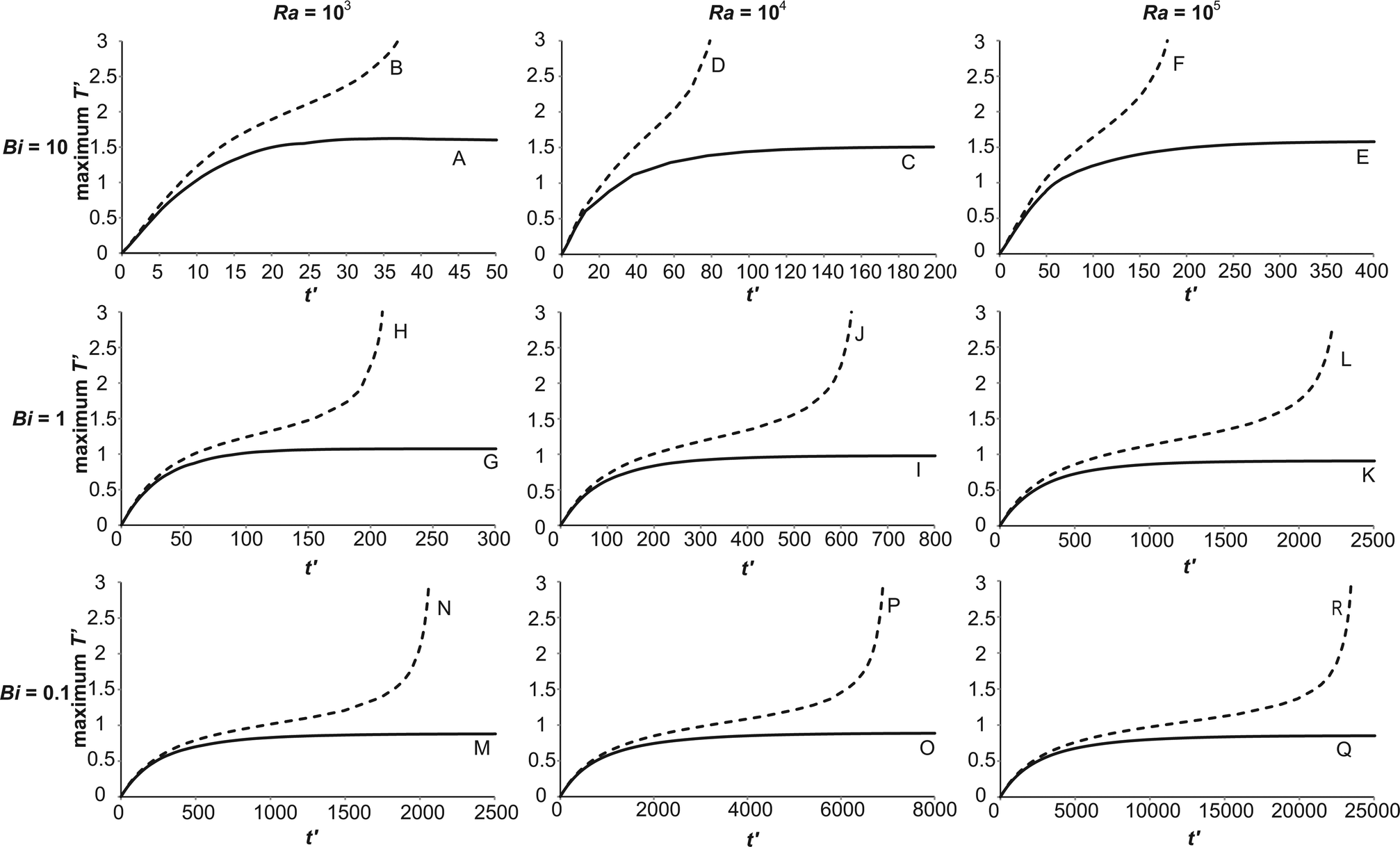
The inclusion of an external heat transfer resistance alters the heat removal from the system. Additionally, the temperature of the wall is no longer constant throughout the duration of the reaction. Both of these factors may alter the way the reaction proceeds, and hence the spatial structures within the reactor. To investigate this difference, eighteen simulations were run to examine the difference between stable and explosive reactions at three different values of Bi. The values considered are Bi = 10 (where external heat transfer is significant, but internal resistances still dominate overall), Bi = 1 (where internal and external thermal resistances are similar in magnitude) and Bi = 0.1 (where external heat transfer is the dominant mechanism). Additionally, three intensities of natural convection, as characterised by Ra (calculated viaeqn (17)) were considered: Ra = 103, where natural convection is becoming important, Ra = 104, where laminar convection is dominant and Ra = 105, where the system is approaching the transition to turbulence. The conditions for the eighteen cases (A–R) are summarised in Table 1. Plotted in Fig. 2 are the temporal developments of the maximum dimensionless temperatures in the reactor for each of cases A–R. For Bi = 10, it is clear that the temporal development of the stable cases (A, C and E) is remarkably similar. In each case, the temperature rises at a relatively constant rate initially, before the rate of increase slows as the natural convection develops and enhances heat removal. When convection becomes fully established, the maximum temperature reaches its steady value. In all three cases the maximum value at steady state is T′ ∼ 1.5. The explosive cases (B, D and F) show a similar rise in temperature to the non-explosive cases initially. Unsurprisingly, after this initial period, the maximum temperature in the vessel is higher than is the case for the stable reactions. In all three cases there is clearly a decrease in the slope of the temperature versus time curve (i.e. ∂2T′/∂t′2 < 0) before an upward inflection in the curve, after which the temperature increases without bound. Such a shape of curve is, of course, characteristic of an explosive system in which reactant consumption is ignored. If consumption of reactant was important, then the increase in temperature would remain bounded, due to the limited heat production by the reaction of a finite mass. In each case, the inflection in temperature can be seen to occur when T′ is in the range 1.5–2. It has been noted previously,10 that this upward inflection in temperature, which is often used to define whether or not an explosion has occurred, can be seen in non-explosive cases when natural convection is important. In particular, it is characteristic of cases where significant reaction occurs before natural convection has been established, and once the flow is significant, the heat removal at the wall increases and thus stabilises the reaction. It is worth pointing out, however, that the observation of such non-explosive inflections occurred in the temperature histories of fixed points in the reactor rather than the overall maximum plotted here. It may be that this procedure, which allows for the migration of the location of the maximum temperature as the reaction proceeds, means that such non-explosive inflections are not seen. It is also interesting to note that the dimensionless time to explosion increases with increasing Ra. An elegant analysis of localised explosion and convection, which should be independent of geometry and boundary conditions, has been preformed,18 and analytical expressions for the transitions between convective and non-convective explosive cases, and the time for the onset of convection developed; however, the time for onset of convection and explosion, and comparison with the analytical expressions developed have not been considered further here.
Table 1 The eighteen cases considered in Fig. 2 and 3. The constant physico-chemical parameters used appear in Section 3. The dimensionless groups τH/τC and τH/τD, which locate a point on the regime diagram in Fig. 1, were varied by changing g and κ respectively. The values of these ratios were chosen to give Ra = 103, 104 or 105, as found using eqn (17). The Biot number was chosen by varying h. The cases A–R are separated into stable reactions (S) and explosive reactions (E)
| Case |

|

|
Bi |
Ra |
State |
| A |
9.5 |
0.300 |
10 |
103 |
S |
| B |
8.7 |
0.275 |
E |
| C |
22.7 |
0.227 |
104 |
S |
| D |
20.5 |
0.205 |
E |
| E |
55 |
0.174 |
105 |
S |
| F |
50 |
0.158 |
E |
|
|
| G |
34.5 |
1.09 |
1 |
103 |
S |
| H |
32.5 |
1.02 |
E |
| I |
106 |
1.06 |
104 |
S |
| J |
98 |
0.98 |
E |
| K |
325 |
1.03 |
105 |
S |
| L |
300 |
0.949 |
E |
|
|
| M |
290 |
9.17 |
0.1 |
103 |
S |
| N |
275 |
8.69 |
E |
| O |
915 |
9.15 |
104 |
S |
| P |
870 |
8.7 |
E |
| Q |
2900 |
9.17 |
105 |
S |
| R |
2750 |
8.70 |
E |
 |
| | Fig. 2 The temporal evolution of the maximum dimensionless temperature in the reactor for cases A–R. These cases fall either side, but close to, the explosion boundary. The stable reactions are plotted as solid lines, whilst the explosive cases are dashed lines. The plots are ordered such that Bi is constant along a row and Ra is constant along a column. The three values of Bi considered are 10, 1 and 0.1, whilst the three values of Ra are 103, 104 and 105. | |
Similar trends are evident when comparing the stable and explosive cases for reduced values of Bi. For Bi = 1, the shapes of the stable cases (G, I and K) and the explosive cases (H, J and L) are very similar for the three values of Ra, with the only obvious quantitative difference being the time taken to reach the stable steady state or the upward inflection which indicates that the system is proceeding to explosion. The time for both increases with increasing Ra as was the case for Bi = 10. When compared with the cases for Bi = 10, it is evident that the temperatures in cases G–L are lower than those in A–F. Specifically, the upward inflection in the temperature occurs at T′ ∼ 1.5 for cases H, J and L and the maximum temperature in the stable cases G, I and K is T′ ∼ 1. This makes intuitive sense as the increasing levels of external resistance to heat transfer as Bi decreases mean that the ability to remove heat from the system is reduced and hence, the reaction will run away at lower temperatures. Additionally, comparison of cases A–F and G–L indicates that the dimensionless timescales for the onset of explosion or the establishment of the steady state are increased as Bi is decreased.
When Bi = 0.1, i.e. when the heat transfer is largely controlled by the external resistance, the behaviours seen in the stable (M, O and Q) and explosive (N, P and R) cases are again similar to those described above. The temperature at which the upward inflection is seen is lower than in those cases with higher Bi and the maximum temperature of the stable systems is once again T′ ∼ 1. Therefore, comparison of all nine explosive cases and all nine stable cases reveals that the evolution of the maximum temperature in the vessel is qualitatively similar across the range of Bi and Ra considered. The most obvious quantitative difference is that the temperatures seen, both at the point where the explosive reaction accelerates to infinity and in the maximum temperature of the stable system, are smaller as Bi is increased, but remarkably similar as Ra is varied at fixed Bi.
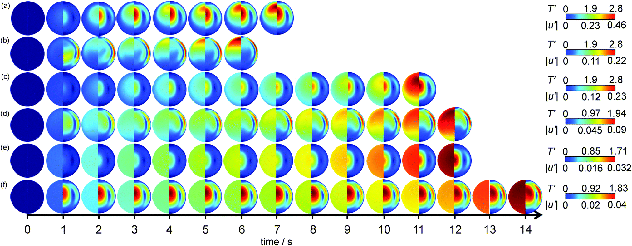
It is clear from Fig. 2 that temporal development of the maximum temperature in the vessel is affected very little by either Bi or Ra, with the primary quantitative difference being in the magnitude of the temperatures observed. It is, however, to be expected that the spatial development of the temperature, and hence velocity fields will be more significantly altered by the existence of external heat transfer. Plotted in Fig. 3 are the spatial variations of the temperature and speed of the flow as explosive reactions proceed. Specifically, cases B, F, H, L, N and R are presented, i.e. the explosive cases for Bi = 10, 1 and 0.1 with Ra = 103 and 105.
 |
| | Fig. 3 The temporal development of the spatial dimensionless temperature (left semi-circle) and speed (right semi-circle) profiles in the reactor for (a) case B (Bi = 10, Ra = 103), (b) case F (Bi = 10, Ra = 105), (c) case H (Bi = 1, Ra = 103), (d) case L (Bi = 1, Ra = 105), (e) case N (Bi = 0.1, Ra = 103) and (f) case R (Bi = 0.1, Ra = 105). The times are given in dimensional units for ease of comparison and indicative colour scales are given on the right. | |
Fig. 3(a) shows case B, which has Bi = 10 and Ra = 103. It is clear that the system heats up due to the reaction and a hot zone begins to form above the centre of the reactor at t = 2 s. In this case there is weak natural convection and this is what displaces the hot zone towards the top of the reactor. As the gas heats up, its density decreases and the higher temperature, lower density gas near the centre of the reactor experiences buoyancy forces which cause it to move vertically upwards. This high speed zone at the centre of the reactor is evident for t > 2 s. As the hot gas moves vertically upwards it contacts the cold wall and hence begins to descend, cooling further as it goes. This moderately high speed gas descending near the wall is also evident in Fig. 3(a). In the bottom half of the reactor, the density gradients are intrinsically stable and so the buoyancy forces are small, as are the velocities. There is also a large region of relatively cold gas, in fact close to the initial temperature, near the bottom of the reactor. As the reaction proceeds, the hot spot in the reactor shifts further up the vertical axis and eventually the explosion initiates in this hot region. There is evidence for all times shown in Fig. 3(a) of a thin thermal boundary layer at the top of the vessel which remains close to the initial temperature. This is despite the fact that the wall temperature is no longer held constant due to the existence of external heat transfer.
Shown in Fig. 3(b) is case F, where Bi = 10 and Ra = 105. It can be seen that the temperature in the vessel increases relatively uniformly over the first second of reaction, and thereafter a hot zone forms close to the top of the vessel. This hot zone can be seen to develop for t > 2 s. As the convection is much more intense than that shown in Fig. 3(a), the hot zone is much closer to the top of the reactor. Additionally, the familiar horizontal stratification of the temperature, which is characteristic of cases when natural convection is significant, is evident. Due to the more intense convection and the proximity of the hot zone to the top of the reactor, the thermal boundary layer at a temperature close to the initial temperature, as seen in Fig. 3(a) for all times, persists only for the first 3 s of reaction. After that, it is evident that the intense natural convection, coupled to the removal of heat externally leads to the wall of the vessel heating up. The speed profiles show that as the vessel warms uniformly at the beginning of the reaction, there is significant upflow around the centreline of the reactor, and the warm gas descending along the cold walls moves very rapidly. Indeed, Fig. 3(b) shows that the flow in the thin layer close to the wall is very fast compared to the central up flow for t > 2 s. These temperature and velocity fields are structurally very similar to those presented previously10 for explosive cases with a constant wall temperature. This is perhaps unsurprising given that when Bi = 10, the internal heat transfer will still largely control the overall heat transfer. As mentioned above, the principal difference between Fig. 3(a) and (b) and their constant wall temperature counterparts is the erosion of the thermal boundary layer near the top of the vessel, due to the variation in the wall temperature that accompanies the external heat loss.
If the heat transfer coefficient describing heat loss from the external wall is decreased, then Bi will also decrease. Shown in Fig. 3(c) is the case where Bi = 1 and Ra = 103i.e. the internal and external heat transfer resistances are of similar order and natural convection is just becoming significant. The temporal development of the temperature shows a similar pattern to that in Fig. 3(a), with the temperature increasing approximately uniformly over the entire cross section of the reactor over the first 2 seconds of reaction before a hot zone develops above the centre of the reactor due to the effects of the convection. The location of this hot zone is similar to that in Fig. 3(a), which is to be expected given the similar intensities of natural convection. The shape of the temperature contours is also qualitatively similar in the two cases. Where Fig. 3(a) and (c) differ though is in the magnitude of the temperature gradients. Whilst the case with Bi = 10 in Fig. 3(a) shows a cold zone, with a temperature close to its initial value, toward the bottom of the reactor and around the wall, when Bi is decreased in Fig. 3(c) then these regions show significant warming. There is therefore still spatial variation in the temperature in this case, but the gradients are considerably smaller. If the development of the velocity field is examined there is again some similarity to what is seen in Fig. 3(a)i.e. there is an area of higher speed that develops in the centre of the reactor after approximately 1 s of reaction and a region of higher speed flow near the wall. It is interesting to note that this downflow close to the wall takes longer to develop in this case than it does for the higher Bi case. This is most likely due to the fact that the wall temperature is much larger in case H in Fig. 3(c) than in case B in Fig. 3(a) and therefore the descending gas is cooled less and so is less dense than in case B and hence there is less of a buoyancy driving force for downflow.
Fig. 3(d) shows the development of temperature and speed for case L, where Bi = 1 and Ra = 105. It can be seen from Fig. 3(d) that the temperature increases virtually uniformly over the entire cross section of the reactor for the first 3 s, with only a small cold zone existing toward the bottom of the reactor. Subsequently, the hot zone begins to develop close to the top of the reactor. Its location is very similar to that seen in Fig. 3(b) for Bi = 10, but as was the case for the low Ra system at Bi = 1, the variation in temperature throughout the reactor is much less than in the higher Bi cases. Thus, the hot zone in Fig. 3(d) (e.g. at t = 12 s) is much larger than that seen in Fig. 3(b) (e.g. at t = 6 s). The development of the speed in Fig. 3(d) in comparison to that in Fig. 3(b) is also interesting. In both cases after ∼1 s a region of relatively strong upflow develops about the centreline. Subsequently, a region of faster downflow along the wall in the upper half of the vessel emerges. It is interesting to note that the extent of this region is much less in the case of Bi = 1 in Fig. 3(d) than when Bi = 10 in Fig. 3(b). As discussed above, this is most likely due to the higher wall temperature that exists in the lower Bi case. As the flow field develops in Fig. 3(d) it is clear that flow near the vertical axis in the top half of the vessel is more significant than was the case for Bi = 10.
Fig. 3(e) shows case N where Bi = 0.1 and Ra = 103. When Bi ≪ 1, the temperature within the system is expected to be approximately spatially uniform.29 It is evident from Fig. 3(e) that this is indeed the case. Virtually no gradients in the temperature are visible. The development of the speed is similar to the previous cases with Ra = 103 in that there is a higher speed region around the centreline. It can be seen that this region is not however shifted towards the top of the reactor as is the case in Fig. 3(a) and (c). This is obviously because there is not a hot zone formed above the centre of the reactor, rather the temperature is uniform over the whole cross section. In Fig. 3(f) is plotted case R with Bi = 0.1 and Ra = 105. As in the low Ra case, the temperature can be seen to develop similarly across the entire cross section. The velocity field is established in the first second of reaction and then changes very little. The intense mixing of course contributes to the spatial uniformity in temperature.
4.2 The effect of Bi on the maximum temperature in a stable system
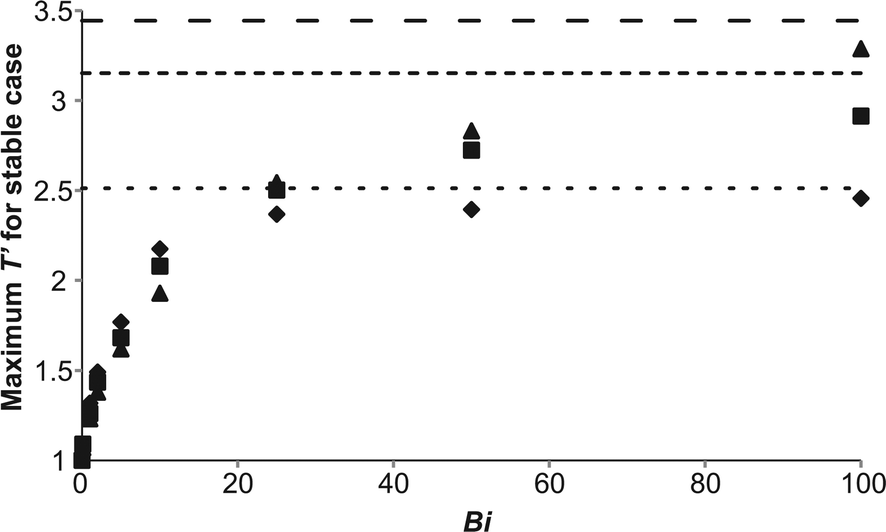
It was shown above that the primary difference between the temporal developments of the maximum temperature in stable systems as Bi varied was the final temperatures reached, with lower temperatures occurring for lower values of Bi. There also seemed to be little difference between the cases at fixed Bi as Ra varied. To elucidate further these effects, simulations were performed to capture the maximum temperature that occurs in the steady state for a stable solution on the explosion boundary (such as is shown in Fig. 1). This was done for a range of Bi and at three values of Ra, i.e. 103, 104 and 105. The results are plotted in Fig. 4. When Bi = 0, the system is perfectly mixed and as predicted by Semenov,1 the maximum dimensionless temperature of a stable system is 1. When Bi is increased, it is clear that there is an increase in the maximum temperature that can be achieved before explosion occurs. Indeed, for Bi > 5, for the range of Ra considered, it can be seen that the maximum temperature rises above the value of 1.6 that was predicted by Frank-Kamenetskii2 for a purely diffusive system. For each Ra when Bi < ∼10 there is very little difference in the maximum temperatures achievable in a non-explosive case. What is interesting to note, however, is that the maximum temperature for each Bi in this range is actually seen for the lowest value of Ra. This result is somewhat counterintuitive and will be discussed further below. Of course, it should be borne in mind that these maximum temperatures were derived numerically and the maximum temperature is sensitive to the proximity to the explosion boundary, nevertheless the trend is evident for all Bi < 10. This trend is reversed as Bi increases above 20, where the increased intensity of convection indicated by a larger Ra results in a higher temperature being achieved in a stable reaction. When Bi increases above 25, the maximum temperatures achieved diverge and the effect of the more intense convection is obvious. The maximum temperatures then clearly approach the values achieved in a constant wall temperature case (i.e. Bi = ∞) asymptotically. Thus, for Ra = 103, the maximum temperature is approximately 2.5, for Ra = 104 it is 3.15 and for Ra = 105 it is 3.45. Unsurprisingly, all three values are comfortably above the value of 1.6 suggested for diffusive systems,2 with a higher temperature being possible in a system with strong convection, due to the improved heat removal. Interestingly, all three values are below the T′ = 5 threshold suggested11 as a criterion for explosion in systems with considerable consumption of reactant. The most important consequence of the variation of the maximum temperature in a stable system with Bi is that a simple criterion for explosion, based on a constant value of dimensionless temperature, may be inappropriate for cases with external heat transfer. This is a topic which clearly merits further study, when systems with significant consumption of reactant are investigated.
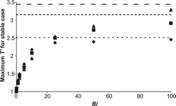 |
| | Fig. 4 The maximum temperature in the reactor at steady state found numerically for a stable system on the explosion boundary as a function of Bi and Ra. The diamonds are for cases with Ra = 103, the squares represent Ra = 104 and the triangles are Ra = 105. Also plotted are horizontal lines which show the maximum temperatures for non-explosive cases with a constant wall temperature (i.e. Bi = ∞). The dotted line is for Ra = 103, the dashed line for Ra = 104 and the open dashed line for Ra = 105. | |
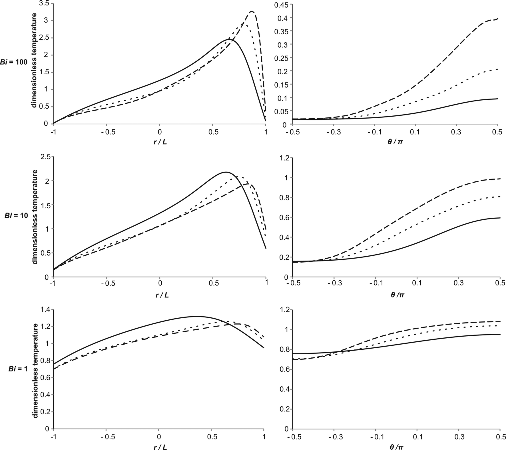
As remarked upon above, there is a shift in the relative values of the maximum dimensionless temperature for stable cases with fixed Ra from the temperatures being very similar, but with the maximum occurring at the lowest value of Ra considered, at low Bi to those with the maximum temperature being observed for the highest value of Ra when Bi > ∼20. To investigate this further, nine simulations were performed for cases very close to the explosion boundary, but in the stable region, for Bi = 1, 10 and 100 with Ra = 103, 104 and 105. A summary of the conditions used for these simulations appears in Table 2. Shown in Fig. 5 are the temperature profiles along the vertical axis and around the surface of the vessel at steady state for each of the nine cases considered. For Bi = 100, it can be seen that the vertical profiles are very similar to those seen, both numerically19 and experimentally,5 when the wall is held at a fixed temperature. The bottom surface of the reactor remains close to its original temperature, and a skewed temperature profile develops, with the point of maximum temperature occurring well above the centre of the reactor. Indeed, as Ra increases and the convection becomes more intense, the point of maximum shifts closer to the top of the vessel, and the increased heat removal leads to a higher temperature in the hot zone. It can also be seen that the difference in temperature between the hot zone and the wall, which is the driving force for heat transfer, is largest for the highest Ra. When considering the surface temperature it can be seen that there is significant variation in temperature around the vertical circumference of the reactor. This is despite the fact that Bi = 100 implies that internal heat transfer is dominant. As one would expect, the temperature of the surface increases monotonically from the bottom towards the top, with the highest temperature occurring at the very top of the reactor. There is very little variation in the surface temperature in the bottom half of the reactor, whereas the hot gas that has passed through the hot zone and cools as it descends along the wall causes a more significant increase in the temperature in the top half of the vessel. Clearly also the more intense the convection, the more heat is transferred to the surface and hence the hotter the surface becomes. It should also be noted that although there is significant variation in the surface temperature upon moving from the bottom to the top of the reactor, the maximum dimensionless surface temperature is an order of magnitude smaller than that in the hot zone of the reactor.
Table 2 Summary of the conditions for the simulations presented in Fig. 5 and 6 for stable cases on the explosion boundary with Bi = 1, 10 or 100 and Ra = 103, 104 or 105
|

|

|
Bi |
Ra |
| 6.8 |
0.215 |
100 |
103 |
| 13.7 |
0.137 |
104 |
| 26.75 |
0.0846 |
105 |
|
|
| 9.1 |
0.288 |
10 |
103 |
| 21.85 |
0.219 |
104 |
| 53.95 |
0.171 |
105 |
|
|
| 33.75 |
1.067 |
1 |
103 |
| 102.35 |
1.024 |
104 |
| 310.9 |
0.983 |
105 |
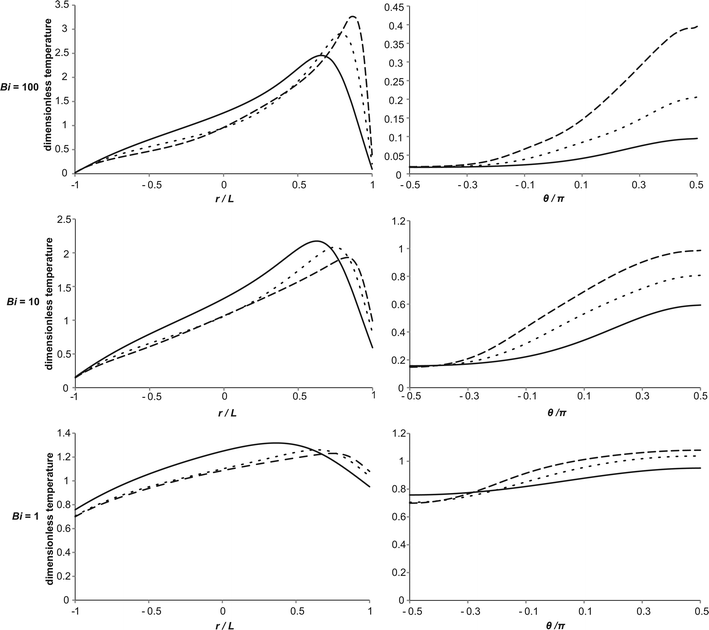 |
| | Fig. 5 The variation in the vertical temperature profile (left column) and the surface temperature (right column) at steady state for stable reactions very close to the explosion boundary. For the vertical profiles, the origin is taken as the centre of the vessel, and the location on the surface of the vessel is represented by the positive angle (θ), measured anti-clockwise from the horizontal axis of the reactor. The conditions used are summarised in Table 2. The horizontal pairs correspond to simulations at constant Bi, with values taken as 100, 10 or 1. In each case the solid line represents Ra = 103, the dotted line Ra = 104 and the dashed line Ra = 105. | |
When considering the cases with Bi = 10, it is evident that there are many qualitative similarities between the vertical and surface temperature profiles and their counterparts for Bi = 100. Considering first the vertical profile, the lowest temperature can be seen at the bottom of the reactor and the hot spot is located above the centre and shifts upwards with Ra. Indeed, it can be seen that the location of the hot spot for each Ra is in a very similar location to those when Bi = 100. When comparing the cases for Bi = 10 and Bi = 100 it is obvious from Fig. 5 that the temperature of the bottom of the reactor is increased only very slightly when Bi is reduced from 100 to 10. There is clearly a much more significant increase in the temperature at the top surface of the reactor for Bi = 10. Additionally, when Bi = 10, as described above, the maximum temperature that is achieved in a stable system decreases with increasing Ra, although the values are much closer together than is the case when Bi = 100.
When Bi is reduced to 1 then internal and external resistances to heat transfer are of similar order. This has the clear effect of making the temperature both within, and on the surface of the reactor much more uniform. The skewed vertical profile is still evident, but the gradients are clearly much smaller, due to the higher surface temperatures. The reduction in temperature difference between the hot zone and the vessel walls means that there is a lower driving force for heat transfer and hence lower temperatures than those seen in the high Bi cases can be sustained without explosion. Whilst the spatial location of the hot spot in the reactor as a function of Ra is very similar for Bi = 100 and 10, the hot zone occurs lower down the vertical axis when Bi = 1, indicating the reduced significance of the flow due to natural convection. Once again, the maximum temperatures on the vertical axis decrease with increased Ra as do the temperature differences between the hot zone and the top surface. When considering the surface temperature, it is clear that the most significant change upon decreasing Bi from 10 to 1 is in the temperature distribution in the bottom half of the reactor. The surface temperatures in the top half change comparatively little, whereas those in the bottom half increase markedly, to give a more uniform profile.
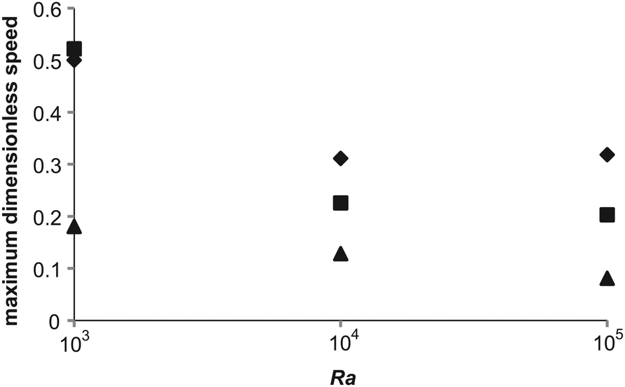
To further investigate the effect of varying Bi on the intensity of convection, and hence the ability to remove heat from the system, the maximum dimensionless speed in each of the nine cases described in Table 2 was plotted as a function of Ra in Fig. 6. For each Bi it is clear that the value of the dimensionless speed is the largest when Ra = 1000; however, it should be noted that this is most likely due to the fact that the scale used for velocity assumes that convection is dominant, whereas for Ra = 1000, diffusive processes will still play a significant role. For the larger values of Ra it is obvious that the maximum dimensionless speed in the reactor at steady state decreases as Bi increases. For the case with Bi = 10 and 1, the maximum speed decreases slightly as Ra is increased from 104 to 105. This is in contrast to the Bi = 100 cases where the maximum speed increases very slightly upon a similar increase in Ra. These observations may indicate that Ra as defined in eqn (17) does not give a true reflection of the intensity of convection in cases where the wall temperature is changing (i.e. cases with smaller Bi). This may also go some of the way to explaining the trends in maximum temperature (i.e. the maximum temperature of a stable system decreases with Ra for low Bi and increases with Ra at high Bi) discussed above.
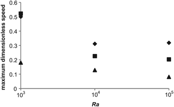 |
| | Fig. 6 The maximum dimensionless speed at steady state for the nine stable cases, close to the explosion boundary, described in Table 2. The diamonds represent those cases with Bi = 100, the squares are cases with Bi = 10 and the triangles are those with Bi = 1. | |
4.3 Identification of explosive conditions as Bi varies
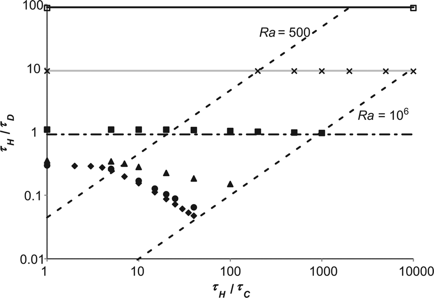
As has been shown above, the variation of external heat transfer, characterised by Bi, can have a significant effect on the behaviour of an exothermic reaction under the influence of natural convection. Of course, one of the most important questions that must be addressed is what effect does this external heat transfer resistance have on the tendency of a system to explode? To investigate this, many simulations were performed to find the boundaries of the explosive region for different values of Bi. These limits are summarised in Fig. 7, which shows a regime diagram, such as presented in Fig. 1, plotted on logarithmic scales. The boundary for Bi = ∞ is the same as that shown in Fig. 1, and agrees well with previous studies.10 The region below the boundary is where explosions occur, and that above it represents stable reactions. Two regions of behaviour are shown very clearly in Fig. 7. For Ra < 500, diffusion dominates and the explosion limit is approximately constant. For Ra > ∼1000, then natural convection is important and there is clearly a power law variation in the explosion limit of the form| |  | (18) |
where Liu et al.10,11 found this exponent to be −0.74 for 500 < Ra < 106. The value found in this work is −0.82, which agrees reasonably well given the precision with which the boundary was found previously. Simulations for Ra > 106 (i.e. turbulent flows) have not been considered here, although the value of the exponent α has been predicted analytically10 to be −2.
 |
| | Fig. 7 The regime diagram for explosion showing the numerically derived explosion limits (for Ra < 106) for a range of Bi. Also shown are two dashed lines which show constant values of Ra. The diamonds show the limit for Bi = ∞, the circles show Bi = 100, the triangles Bi = 10, the filled squares Bi = 1, the crosses Bi = 0.1 and the open squares Bi = 0.01. The horizontal lines show Semenov's prediction, viaeqn (20), for the explosive limit in a well-mixed system with varying Bi. The dot-dash line shows eqn (20) for Bi = 1, the grey line Bi = 0.1 and the black line Bi = 0.01. | |
When a small amount of external heat transfer is allowed for (i.e. when Bi = 100), it can be seen that for Ra < 500, the explosion limit is virtually identical to that for the constant wall temperature case. As Ra increases above 500 and natural convection becomes more significant, it can be seen that explosions occur at a slightly higher value of τH/τD than when Bi = ∞. This is of course due to the fact that the external resistance to heat transfer lessens somewhat the stabilising effect of the increased fluid flow and hence heat transfer from the contents of the vessel to the wall. It is also evident that the power law behaviour described in eqn (18) still exists, though the value of the exponent is reduced.
For Bi = 10 it is shown in Fig. 7 that the critical value of τH/τD in the diffusive region is increased slightly and that the stabilising effect of convection has been substantially lessened. For Bi = 1, there is still a very slight stabilising effect of convection evident for 500 < Ra < 106, however for Bi < 1, the explosive limit has an approximately constant value of τH/τD. It is shown very clearly in Fig. 7 that external heat transfer has two main effects viz. it increases the critical value of τH/τD indicating that the system is more prone to explode and it also lessens the stabilising effect of natural convection.
The extent to which the stabilising effect of convection is suppressed can be characterised by the exponent in eqn (18). The variation of this exponent is shown, as derived from a best-fit of the numerical results, in Fig. 8. Clearly, when Bi is very small, the explosive limit is approximately constant so α is close to zero. The bulk of the variation in α is seen over the range 1 < Bi < 100, which is similar to the range reported for main effect of Bi on explosion in diffusive systems with consumption of reactant.16 For Bi > 100, the value of the exponent in eqn (18) approaches the Bi = ∞ value asymptotically.
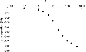 |
| | Fig. 8 The exponent in eqn (18), which characterises the stabilising effect of natural convection on the system, as a function of Bi. | |
4.4 The Frank-Kamenetskii and Semenov limits
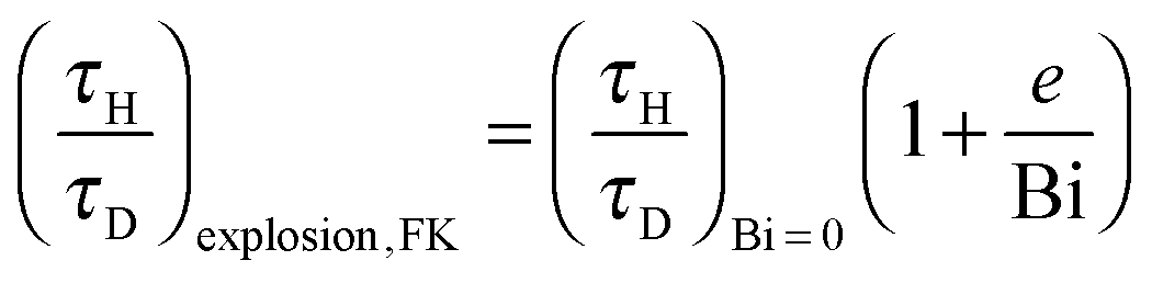
The numerically derived explosion limits presented in Fig. 8 can be compared to analytical solutions in the Frank-Kamenetskii and Semenov limits. Frank-Kamenteskii derived2 an approximate expression for the transition to explosion which can be written as| |  | (19) |
Plotted in Fig. 9 are the numerically derived explosive limits for a purely diffusive system and a line representing eqn (19). There is clearly an excellent agreement between Frank-Kamenetskii's prediction and the numerical results. As observed above, the value of τH/τD at the explosive limit is approximately constant for Bi > 10 and as predicted by eqn (19)τH/τD is proportional to Bi−1 as Bi tends to zero and hence 1 + e/Bi tends to e/Bi.
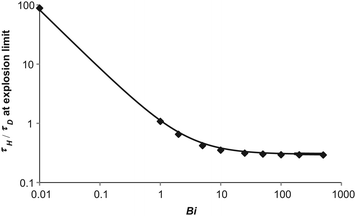 |
| | Fig. 9 A comparison of the numerically derived explosion limit for a purely diffusive system for different values of Bi with Frank-Kamenetskii's approximate expression in eqn (19). The diamonds are the numerically derived limits and the solid line represents eqn (19). | |
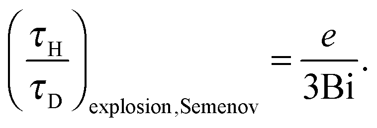
At small values of Bi, where external heat transfer is the dominant mechanism, the Semenov limit of a well-mixed system is approached. Eqn (1) can be re-written in terms of the characteristic timescales used here as
| | 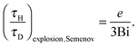 | (20) |
Eqn (20) is plotted for Bi = 0.01, 0.1 and 1 in
Fig. 7. For Bi = 1,
eqn (20) slightly under predicts the explosive limit and, of course, does not capture the marginal stabilising effect of convection. This discrepancy is unsurprising given that there is still some spatial variation in the temperature field, as shown in
Fig. 5. For Bi ≪ 1, the agreement between
eqn (20) and the numerically derived boundaries can be seen to be excellent in
Fig. 7, with the numerically derived results agreeing with Semenov's prediction to within 2%. This excellent agreement between the analytical predictions in both limits not only provides further validation of the numerical methods used, but also shows that the inclusion of external heat transfer in systems with natural convection truly bridges these two classical limits.
5. Conclusions
The behaviour of an exothermic chemical reaction occurring in a spherical vessel under the influence of natural convection and an external heat transfer resistance, but without consumption of reactant, has been studied numerically. It has been shown that the external heat transfer, as characterised by a Biot number, has very little qualitative impact on the temporal development of the maximum temperature in the reactor during explosive and non-explosive reactions. The main quantitative effect is that the reactions take place at a lower temperature when Bi is reduced. Indeed, it has been shown that the maximum dimensionless temperature achieved in a non-explosive reaction on the explosion boundary increases from 1 in the well mixed limit to its constant wall temperature value asymptotically. For Bi < ∼10, the maximum temperature varies little with Rayleigh number, but interestingly is lower for higher values of Ra. This is in contrast to what is observed at higher Bi where more intense natural convection means that higher temperatures can be sustained in non-explosive cases. This effect may be due to the reduction in driving force for heat transfer from the hot zone of the reactor to the wall. This is primarily due to the fact that the wall temperature increases much more significantly as Bi is reduced. Importantly, this variation in maximum temperature achieved in stable systems means that explosion criteria based on the maximum temperature achieved in the reactor may be inappropriate for systems with significant external heat transfer.
A region of parameter space where explosions occur has been defined for a series of values of Bi. It has clearly been shown that the inclusion of external heat transfer means that the region of parameter space where explosions occur is larger and that the stabilising effect of natural convection on the reaction is greatly diminished as Bi is reduced, particularly over the range 100–1. Finally, the numerical results have been shown to agree very well with the analytical solutions of Frank-Kamenetskii and Semenov in the purely diffusive and well-mixed limits.
7. Nomenclature
| Bi | Biot number, Bi = hL/kT |
|
c
| concentration of reactant |
|
c′ | dimensionless concentration of reactant, c′ = c/c0 |
|
c
0
| initial concentration of reactant |
|
C
P
| specific heat at constant pressure |
|
D
C
| diffusion coefficient of reactant |
|
E
| activation energy |
|
g
| acceleration due to gravity |
|
h
| external heat transfer coefficient |
|
k
| rate constant |
|
k
0
| rate constant evaluated at T = T0 |
|
k
T
| thermal conductivity |
|
L
| characteristic length (radius) of the reactor |
| Le | Lewis number, Le = κ/DC |
|
n
| order of the reaction |
|
P
| pressure |
|
P
0
| initial pressure |
|
P′ | dimensionless pressure, P′ = (P − P0)/ρ0U2 |
| Pr | Prandtl number, Pr = ν/κ |
|
q
| exothermicity of the reaction |
|
r
| radial coordinate |
|
R
| universal gas constant |
| Ra | Rayleigh number, Ra = βgL3ΔT/κν |
|
S
v
| surface area per unit volume |
|
t
| time |
|
t′ | dimensionless time, t′ = Ut/L |
|
T
| temperature |
|
T′ | dimensionless rise in temperature, T′ = E(T − T0)/RT02 |
|
T
ad′ | dimensionless adiabatic temperature increase, Tad′ = qc0E/(ρ0CPRT02) |
|
T
0
| constant temperature of the environment |
|
| velocity |
|
′ | dimensionless velocity, ′ = /U |
|
U
| characteristic velocity |
|
| spatial coordinates |
|
′ | dimensionless spatial coordinates, x′ = x/L |
|
Z
| pre-exponential factor in the Arrhenius term |
|
β
| coefficient of thermal expansion |
|
δ
| Frank-Kamenetskii parameter, δ = L2k0cn0qE/κρ0CPRT02 |
| ΔT | characteristic temperature increase, ΔT = RT02/E |
|
η
| dimensionless parameter, η = RT0/E |
|
θ
| angle measured anti-clockwise from the horizontal axis of the reactor |
|
κ
| thermal diffusivity |
|
μ
| viscosity |
|
ν
| kinematic viscosity |
|
ρ
| density |
|
ρ
0
| density at T = T0 |
|
τ
C
| timescale for convection |
|
τ
D
| timescale for diffusion of heat |
|
τ
H
| timescale for heating by reaction |
|
ψ
| Semenov number, ψ = k0cn0qE/hSvRT02 |
Acknowledgements
The financial support of the Engineering and Physical Sciences Research Council via Small Equipment Grant EP/K031317/1 is gratefully acknowledged.
References
- N. N. Semenov, Z. Phys., 1928, 48, 571–582 CrossRef CAS.
-
D. A. Frank-Kamenetskii, in Diffusion and Heat Transfer in Chemical Kinetics, ed. J. P. Appleton, Plenum, 2nd edn, 1969 Search PubMed.
- B. J. Tyler, Combust. Flame, 1966, 10, 90–91 CrossRef CAS.
-
P. G. Ashmore, B. J. Tyler, T. A. B. Wesley, Eleventh Symposium (International) on Combustion, 1967, 1133–1140.
-
W. H. Archer, PhD thesis, University of Manchester Institute of Science and Technology, 1977.
- A. G. Merzhanov and E. A. Shtessel, Combust., Explos. Shock Waves (Engl. Transl.), 1971, 7, 58–65 CrossRef.
- D. R. Jones, Int. J. Heat Mass Transfer, 1973, 16, 157–167 CrossRef CAS.
- E. A. Shtessel, K. V. Priytkova and A. G. Merzhanov, Combust., Explos. Shock Waves (Engl. Transl.), 1971, 7, 137–146 CrossRef.
- A. G. Merzhanov and E. A. Shtessel, Astronaut. Acta, 1973, 18, 191–199 Search PubMed.
- T.-Y. Liu, A. N. Campbell, S. S. S. Cardoso and A. N. Hayhurst, Phys. Chem. Chem. Phys., 2008, 10, 5521–5530 RSC.
- T.-Y. Liu, A. N. Campbell, A. N. Hayhurst and S. S. S. Cardoso, Combust. Flame, 2010, 157, 230–239 CrossRef CAS.
- F. G. de Azevedo, J. F. Griffiths and S. S. S. Cardoso, Combust. Flame, 2014, 161, 1752–1755 CrossRef.
- F. G. de Azevedo, J. F. Griffiths and S. S. S. Cardoso, Phys. Chem. Chem. Phys., 2013, 15, 16713–16724 RSC.
- T.-Y. Liu and S. S. S. Cardoso, Combust. Flame, 2013, 160, 191–203 CrossRef CAS.
- F. G. de Azevedo, J. F. Griffiths and S. S. S. Cardoso, Phys. Chem. Chem. Phys., 2014, 16, 23365–23378 RSC.
- T. Boddington, C. Feng and P. Gray, Proc. R. Soc. A, 1984, 391, 269–294 CrossRef CAS.
-
J. S. Turner, Buoyancy Effects in Fluids, Cambridge University Press, 1979, pp. 207–250 Search PubMed.
- T.-Y. Liu and S. S. S. Cardoso, Phys. Chem. Chem. Phys., 2012, 14, 192–199 RSC.
- A. N. Campbell, S. S. S. Cardoso and A. N. Hayhurst, Chem. Eng. Sci., 2007, 62, 3068–3082 CrossRef CAS.
- T. Dumont, S. Ge'nieys, M. Massot and V. A. Volpert, SIAM J. Appl. Math., 2002, 63, 351–372 CrossRef.
- S. S. S. Cardoso, P. C. Kan, K. K. Savjani, A. N. Hayhurst and J. F. Griffiths, Combust. Flame, 2004, 136, 241–245 CrossRef CAS.
- S. S. S. Cardoso, P. C. Kan, K. K. Savjani, A. N. Hayhurst and J. F. Griffiths, Phys. Chem. Chem. Phys., 2004, 6, 1687–1696 RSC.
- A. N. Campbell, S. S. S. Cardoso and A. N. Hayhurst, Proc. R. Soc. A, 2005, 461, 1999–2020 CrossRef CAS.
- A. N. Campbell, S. S. S. Cardoso and A. N. Hayhurst, Chem. Eng. Res. Des., 2006, 84, 553–561 CrossRef CAS.
- A. N. Campbell, S. S. S. Cardoso and A. N. Hayhurst, Chem. Eng. Sci., 2005, 60, 5705–5717 CrossRef CAS.
- A. N. Campbell, S. S. S. Cardoso and A. N. Hayhurst, Combust. Flame, 2008, 154, 122–142 CrossRef CAS.
- M. R. Foster and H. Pearlman, Combust. Flame, 2008, 147, 108–117 CrossRef.
- M. R. Foster and H. Pearlman, Microgravity Sci. Technol., 2012, 24, 113–125 CrossRef.
-
F. P. Incropera and D. P. DeWitt, Fundamentals of Heat and Mass Transfer, Wiley, 4th edn, 1996, pp. 215–216 Search PubMed.
- COMSOL, COMSOL Multiphysics Reference Guide Version 4.3a, 2012.
- A. N. Campbell, S. S. S. Cardoso and A. N. Hayhurst, Phys. Chem. Chem. Phys., 2006, 8, 2866–2878 RSC.
|
| This journal is © the Owner Societies 2015 |
Click here to see how this site uses Cookies. View our privacy policy here. 
 Open Access Article
 This Open Access Article is licensed under a