Quantifying solvated electrons' delocalization

Abstract

Delocalized, solvated electrons are a topic of much recent interest. We apply the electron delocalization range EDR(r⃑;u) (J. Chem. Phys., 2014, 141, 144104) to quantify the extent to which a solvated electron at point r⃑ in a calculated wavefunction delocalizes over distance u. Calculations on electrons in one-dimensional model cavities illustrate fundamental properties of the EDR. Mean-field calculations on hydrated electrons (H₂O)_n⁻ show that the density-matrix-based EDR reproduces existing molecular-orbital-based measures of delocalization. Correlated calculations on hydrated electrons and electrons in lithium–ammonia clusters illustrates how electron correlation tends to move surface- and cavity-bound electrons onto the cluster or cavity surface. Applications to multiple solvated electrons in lithium–ammonia clusters provide a novel perspective on the interplay of delocalization and strong correlation central to lithium–ammonia solutions' concentration-dependent insulator-to-metal transition. The results motivate continued application of the EDR to simulations of delocalized electrons.

---

I. Introduction

Solvated electrons are a classic chemical system that has attracted much study.¹ Mobile² solvated electrons are responsible for the blue color of dilute lithium–ammonia solutions and the transition to a metallic state seen at high lithium concentrations.^3–5 Hydrated electrons are important intermediates in radiation chemistry and in many biological processes.⁶ Electronic structure calculations have contributed to the understanding of solvated electrons.^4,6–10 Calculated vertical detachment energies (VDEs) for electrons solvated in water clusters (H₂O)_n⁻ suggest^11,12 that experimental photoelectron spectra¹³ may arise from surface-bound electrons. Mixed quantum–classical dynamics simulations suggest models for electrons in bulk water¹⁴ and lithium–ammonia solutions.^15–17 Several recent studies highlight the importance of the quantum–classical interaction potential.^10,18,19 All-electron calculations provide additional insights.^4,20–22Ref. 23 provides a recent perspective on the role of delocalization in electron solvation.

Solvated electrons' behavior depends on the interplay of electron delocalization and electron–electron correlation. Delocalization denotes the nonclassical “coherence” of electrons between different points in space, e.g., the off-diagonal terms in Fig. 1. This off-diagonal delocalization²⁴ is central to covalent bonding and reactivity. Delocalization is particularly important for highly delocalized solvated electrons.²⁵ Correlation denotes all effects excluded from a mean-field (Hartree–Fock, HF) calculation, including dispersion (van der Waals) interactions. Correlation is important for the stability of solvated electrons,^26–35 as well as for lithium–ammonia solutions' transition to the metallic state.^4,36

Fig. 1 γ(x;x′) (left) and EDR(x;u) (right) for boxes containing N = 1, 2, 3, 10 noninteracting spinless Fermions. The red line through the N = 3 points γ(L/3,x′) is discussed in the text.

Existing electronic structure methods can accurately treat solvated electrons' VDE.^27–29,35 However, quantifying solvated electrons' delocalization remains challenging. Most analyses of delocalization are based on the highest occupied molecular orbital (MO) or spin density from a HF or density functional theory (DFT) wavefunction.^4,29 This approach has limitations. MOs are not uniquely defined in many-electron wavefunctions.³⁷ Hartree–Fock MOs and spin densities do not include correlation effects.³⁸ DFT MOs come from a reference system of noninteracting^39,40 or partially interacting⁴¹ Fermions, which is generally more delocalized than the real system. (The exact Kohn–Sham wavefunction is arguably at least as delocalized as the exact interacting wavefunction, because the Kohn–Sham kinetic energy T_s[ρ] is bound by the exact kinetic energy T_s[ρ] ≤ T[ρ].) Attempts to address these limitations include analyses of DFT electron densities,^{15–17,42–44} the electron localization function,^45,46 and nearly-singly-occupied natural orbitals from correlated wavefunctions.^{34,35,47–49} New tools to quantify delocalization could complement and extend this work.

We recently proposed the electron delocalization range (EDR) to quantify and visualize electron delocalization.⁵⁰ The EDR is based on the nonlocal one-particle density matrix γ(r⃑,r⃑′) of a calculated N-electron wavefunction Ψ(r⃑₁,r⃑₂…r⃑_N),

γ(r⃑,r⃑′) ≡ N∫d³r⃑₂…d³r⃑_NΨ(r⃑,r⃑₂…r⃑_N)Ψ*(r⃑′,r⃑₂…r⃑_N). (1)

(Spin and time dependence are suppressed throughout. All calculations treat approximate stationary state solutions of Schrödinger's equation.) γ(r⃑,r⃑′) gives the probability that an electron delocalizes between points r⃑ and r⃑′. Diagonal elements lim_{r⃑′→r⃑}γ(r⃑,r⃑′) = ρ(r⃑) give the probability density for finding an electron at r⃑. Bonding interactions between atoms A and B typically correspond to γ(r⃑ ∈ A,r⃑′ ∈ B) > 0. The EDR quantifies the degree to which an electron at r⃑ delocalizes over distance |r⃑ − r⃑′| by contracting γ(r⃑,r⃑′) with a test function of |r⃑ − r⃑′| that decays over some length scale u:

EDR(r⃑,u) = ∫d³r⃑′g_u(r⃑,r⃑′)γ(r⃑,r⃑′) (2)

The prefactors in eqn (3) ensure that the unitless EDR obeys |EDR(r⃑;u)|² ≤ 1. Our choice of a Gaussian test function enables analytic integration over r⃑′ in eqn (2), when the molecular orbitals and γ are expanded in standard atom-centered Gaussian basis sets. Global descriptors of delocalization may be obtained from density–weighed averages

〈EDR(u)〉 = ∫d³r⃑′ρ(r⃑)EDR(r⃑;u), (4)

and differences between two calculations A and B

ΔEDR(A − B;u) = 〈EDR(u)〉(A) − 〈EDR(u)〉(B). (5)

Our previous work showed that the EDR effectively characterizes the delocalization of electrons across multiple length scales.⁵⁰ EDR(r⃑;u) at small distances u ∼ 0.1 Angstrom peaks at points r⃑ in the cores of first-row atoms. EDR(r⃑;u) at larger distances u ∼ 0.5 Angstrom peaks at points r⃑ around the localized lone pairs of, e.g., oxygen atoms. EDR(r⃑;u) at u ∼ 0.6 Angstrom peaks at points r⃑ in C–C and C–H bonds. Calculations on a model cavity-bound hydrated electron^7,8,51 (H₂O)₆⁻ showed that EDR(r⃑;u) at points r⃑ inside the cavity peaked at increasingly large u (from 1.4 Angstrom to 3.3 Angstrom) as the cavity radius increased. Calculations on the strongly correlated electron pair in stretched singlet H₂ showed that the EDR quantifies the interplay of delocalization and strong correlation.^52–57 These preliminary results motivate further exploration of the EDR for solvated electrons.

This work applies the EDR to several problems relevant to solvated electrons. Calculations on simple model systems show how the EDR quantifies “off-diagonal” coherence lengths and electron correlation effects on delocalization. Hartree–Fock calculations on hydrated electrons (H₂O)_n⁻ show that EDR-based descriptors reproduce existing MO-based measures of hydrated electrons' delocalization.²⁹ Correlated calculations on (H₂O)_n⁻ and lithium–ammonia clusters⁴ show that the EDR illustrates localization of surface-bound electrons onto cluster surfaces, and delocalization of cavity-bound electrons onto cavity walls. Calculations on spin-paired diamagnetic species in lithium–ammonia clusters,⁴ and multireference calculations on multiple solvated electrons,^15–17 illustrate the interplay of delocalization and strong correlation relevant to the transition to the metallic state. These results motivate further application of the EDR to delocalized electrons.

II. Computational methods

All molecular calculations use the development version of the Gaussian suite of programs.⁵⁸ The EDR is evaluated using one-particle density matrices from Hartree–Fock, generalized Kohn–Sham density functional theory (DFT),^39,40,59 post-Hartree–Fock, or multireference calculations. Second-order many-body perturbation theory (MP2) and coupled cluster with singles and doubles (CCSD) calculations use the Gaussian default choice of frozen core orbitals. Brückner doubles (BD) calculations^60,61 and complete active space self-consistent field (CASSCF) calculations correlate all electrons. Post-Hartree–Fock density matrices are evaluated using the Z-vector method,^38,62 with Gaussian keyword “Density = Current”. DFT calculations use various approximate exchange–correlation (XC) functionals. These include the local spin-density approximation with Vosko–Wilk–Nusair correlation functional V (LSDA),⁶³ Becke's three-parameter global hybrid incorporating Lee–Yang–Parr correlation (B3LYP),^64–67 the half-and-half global hybrid BHLYP,⁶⁸ and the long-range-corrected hybrid LC-ωPBE.⁶⁹ Molecular calculations on open-shell systems are performed spin-unrestricted unless noted otherwise. Molecular calculations evaluate the EDR as described previously.^50,70 〈EDR(u)〉 is evaluated by numerical integration of eqn (4) using a standard DFT numerical integration grid.⁷¹ The descriptor u_av, discussed below, is obtained from a three-point fit to 〈EDR(u_j)〉 from an even-tempered set of {u_j}.

Pictures of calculated molecular geometries use a “ball-and-stick” description of chemical bonds. For example the O–H bonds in the water clusters of Fig. 4 are drawn as lines between the O and H atoms. These bond orders are included solely as a guide to the eye.

Other details of the individual calculations are as follows. The calculations on 1D systems in Section III A, and some test calculations in Section III B 2, use a Mathematica worksheet provided as ESI.† Calculations on H₂O and H₂O⁻ in Section III A use the aug-cc-pVQZ basis set^72,73 and the anion's HF/aug-cc-pVTZ geometry. Calculations on the (H₂O)_N⁻ clusters in Section III B use the cluster geometries reported in ref. 29, and the 6-31(+,3+)G(d) basis set shown in ref. 27–29 to be suitable for post-Hartree–Fock calculations on hydrated electrons. Calculations on the octahedral (H₂O)₆⁻ Kevan structure^7,8,51 in Sections III B 4–III B 5 use geometries from ref. 51, and rigidly shift each water molecule distance R from the cavity center. Distances are measured from the cavity center to the closest H atom. Calculations combine the 6-31(+,3+)G* basis set on all atoms, and the aug-cc-pVQZ basis functions of hydrogen atom on a “ghost” atom at the cluster center.⁵¹

Calculations on the lithium–ammonia clusters in Section III C use the 6-31(+,3+)G(d) basis set. Cluster geometries are obtained from gas-phase B3LYP/6-31+G(d,p) calculations, based on the clusters in ref. 4, 22 and 74. Spatial symmetry is not enforced in these calculations. Geometries are labeled by their approximate symmetries.

Calculations on the lithium–ammonia clusters of Section III D combine an explicit quantum-mechanical (QM) treatment of six solvated electrons with a molecular mechanics (MM) model of the (NH₃)₂₀ cavity. QM calculations use a basis set defined by fifteen “ghost” atoms evenly spaced along the cavity center. Two s-type Gaussian functions with exponents 0.5 and 0.1 au are centered at each ghost atom. The cavity walls are made up of five rigid square-planar (NH₃)₄ units. Each unit has N–N distances 4.55 Angstrom, taken from the O_h-symmetric e⁻@(NH₃)₈ cavity of ref. 4. H atom positions are taken from a gas-phase PM6⁷⁵ geometry optimization of square-planar (NH₃)₄⁻, constraining the H–N–H groups to lie in a plane and constraining N–N distances to 4.55 Angstrom. This yields reasonable N–H bond lengths 1.02 Angstrom and H–H bond lengths 2.54 Angstrom. The MM calculations replace each H atom in NH₃ with a point charge +0.268; and replace each N atom with a point charge −0.804 and a repulsive s-type Gaussian pseudopotential with exponent 0.45 au and prefactor 1.60 Hartree. CASSCF calculations on this system correlate all 6 electrons using 12 orbitals. The Gaussian input file for the CASSCF calculation is included in the ESI.†

It is often useful to assign global descriptors for the delocalization of a solvated electron or electron pair. We define the delocalization length u_av of the solvated electron in anion M⁻ as the position of the maximum in ΔEDR(M⁻ – M;u), evaluated at the anion M⁻ optimized ground-state geometry. The corresponding total energy difference E(M⁻) − E(M) defines the electron's VDE. The left panel of Fig. 3 below illustrates evaluation of u_av for H₂O⁻. We define u_av of the solvated electron in neutral open-shell Li(NH₃)₄ (Section III C 1) as the position of the maximum in ΔEDR(Li(NH₃)₄ − Li(NH₃)₄⁺;u), and define u_av of the solvated electron pairs in neutral singlet (Li(NH₃)₄)₂ (Section III C 2) as the position of the maximum in ΔEDR([Li(NH₃)₄]₂ − [Li(NH₃)₄]₂²⁺;u). Plots of representative ΔEDR and tables of all species' 〈EDR(u)〉 are included as ESI.† All species' ΔEDR have a single peak giving a unique u_av.

III. Results

A. Model systems

This section shows that the EDR quantifies the off-diagonal cohererence of the one-particle density matrix γ(r⃑,r⃑′), and illustrate how occupancy of highly oscillatory single-particle states (“virtual orbitals”) in correlated wavefunctions tends to reduce the value of the EDR. This effect is important in our subsequent studies of correlation-induced (de)localization of solvated electrons.

We begin by considering a simple 1D model for the solvated electron,^76,77 one or more noninteracting spinless Fermions in a box of length L with infinite walls. One-electron Hamiltonian eigenfunctions are the familiar particle-in-a-box states , 0 ≤ x ≤ L, ψ_m(x) = 0 elsewhere; m = 1, 2, 3,…. The EDR is evaluated with 1D test function g^1D_u(x,x′) = (2/(πu²))^1/4ρ^−1/2(x) exp(−|x − x′|²/u²). This model system allows us to visualize the entire one-particle density matrix γ(x,x′) in 2D contour plots, which can be directly compared to plots of EDR(x;u).

1. Quantifying delocalization with the EDR. Fig. 1 compares contour plots of the real-space γ(x,x′) (left, in blue) and EDR(x;u) (right, in green) for the ground state of 1, 2, 3, and 10 noninteracting spinless Fermions in a box of length L.

The left panels of Fig. 1 plot γ(x,x′) in the box as a function of the unitless relative positions x/L and x′/L. White regions denote large positive values of γ, blue and black regions denote small and negative γ. The density matrix is largest along the diagonal, and decays with increasing off-diagonal separation |x − x′|. The “width” of the density matrix along the antidiagonal corresponds to the electrons' coherence length,⁷⁸i.e., the nonclassical “delocalization” of covalent bonds. Increasing the number of noninteracting Fermions in the box increases the electron density and decreases the off-diagonal delocalization length.

The right panels of Fig. 1 plot EDR(x;u) as a function of the unitless relative position x/L on the abscissa, and the unitless relative delocalization length u/L along the ordinate. White regions denote EDR near one, dark green regions denote EDR near or less than zero. Ref. 50 included similar contour plots of the EDR in molecules. Reduced delocalization, i.e., reduced off-diagonal width of the density matrix, shifts the EDR peaks down to smaller delocalization lengths u. In this sense, the EDR at point x captures the nonclassical off-diagonal delocalization of an electron at point x.

One caveat to the above description is that the EDR can predict long delocalization lengths in low-density regions. For example, the N = 3 EDR peaks at relatively large u in the low-density region x ∼ L/3. We suggest that this occurs because the EDR samples a horizontal (or equivalently vertical) rather than antidiagonal slice through the density matrix. To illustrate, the N = 3 system's EDR(x = L/3;u) is obtained by contracting the test function with the “horizontal slice” of points γ(x = L/3,x′). Fig. 3 highlights this horizontal slice of points in the N = 3 density matrix with a red line. The figure shows that these points connect two of the three lobes in the N = 3 density matrix, leading to a relatively large delocalization length. While we speculate that sampling an “antidiagonal” slice γ(x + s/2,x − s/2) could avoid this effect, implementing the resulting integration would be more complicated than our current approach. Moreover, despite this caveat, the overall trend of Fig. 1 is that the EDR provides a reasonable local measure of off-diagonal density matrix delocalization.

2. Normalization effects on the EDR. One important result in Fig. 1 is that the EDR tends to become smaller as the electron density increases, such that the EDR plots become darker at increasing N. This is a specific case of a more general phenomenon: occupancy of highly oscillatory single-particle orbitals tends to decrease the EDR. This normalization effect can be understood from Fig. 2, which illustrates ρ^−1/2(x)γ(x,x′) and the EDR test function (2/(πu²))^1/4 exp(−|x − x′|²/u²) for the m = 1 and m = 2 particle in a box states. Results are plotted as functions of the EDR integration variable x′. Position x and length scale u are selected to maximize the resulting EDR(x;u). Fig. 2 shows that the normalized test function overlaps the entire the m = 1 γ(r,r′), but overlaps with at most one lobe of the m = 2 γ(r,r′). This reduced overlap reduces the overall value of the EDR. Fig. S1 (ESI†) confirms that 〈EDR(u)〉 decreases at most u values for the m = 2 and m = 3 states of a single particle in a box.

Fig. 2 The two quantities in the integrand of eqn (2), test function (2/(πu²))^1/4 exp(−|x − x′|²/u²) (red) and weighted density matrix ρ^−1/2(x)γ(x,x′) (blue), plotted as a function of integration variable x′. Results are plotted for the m = 1 (solid) and m = 2 (dashed) states of a single particle in a box, with x and u selected to maximize EDR(x;u). The normalized test function overlaps with at most one lobe of the normalized m = 2 density matrix, reducing the maximum value of the EDR.

The normalization effects in Fig. 2 suggest that any process that increases the occupancy of highly oscillatory single-particle states (“virtual orbitals”) will tend to decrease the EDR. Indeed, we have used this effect to distinguish fractional spin⁵⁷ in strongly correlated stretched singlet H₂.⁵⁰ In the present work, our efforts to quantify delocalization in post-Hartree–Fock wavefunctions must account for these normalization effects.

Fig. 3 illustrates this by showing different views of correlation in a second model system, H₂O⁻. (This is not intended to represent a realistic hydrated electron, and is included solely to illustrate computed trends.) The left panel of Fig. 3 shows the difference ΔEDR(anion–neutral;u), used to evaluate our descriptor u_av of the solvated electron's delocalization length. Horizontal lines denote u_av. Correlation binds the solvated electron more tightly and slightly reduces u_av. The right panel of Fig. 3 shows the difference ΔEDR(MP2 − HF;u) between correlated and Hartree–Fock calculations on H₂O and H₂O⁻. ΔEDR(MP2 − HF;u) has a negative peak in the valence region u ∼ 1 bohr, consistent with the normalization effects in Fig. 2. However, the anion also has a significant positive peak in ΔEDR(MP2 − HF;u) at moderate u ∼ 5 bohr, and a negative peak at u ∼ 30 bohr, both of which are consistent with correlation-induced changes in the structure of the bound electron. Overall, the simple u_av descriptor provides a useful measure of correlation effects on localization, though some caution is needed in its interpretation.

Fig. 3 Electron correlation effects on delocalization in H₂O⁻. (left) ΔEDR(anion–neutral;u) for HF and MP2 calculations. Horizontal lines denote the descriptor u_av. (right) ΔEDR(MP2 − HF;u) for H₂O⁻ and neutral H₂O. The normalization effects in Fig. 2 make these curves negative at u = ∼1 bohr.

B. Hydrated electrons

We next consider the EDR's predictions for electrons hydrated in water clusters (H₂O)_n⁻. Such clusters have long been studied for their intrinsic interest and as a model for bulk hydrated electrons.^{6,9–12,27–29} This section shows that the u_av descriptor introduced above, evaluated from Hartree–Fock density matrices, recovers existing MO-based measures of hydrated electrons' delocalization.²⁹ The EDR and u_av from post-HF calculations suggests that correlation tends to localize surface-bound isomers to cluster surfaces, and delocalize cavity-bound isomers from the cavity center to the cavity wall. DFT calculations can recover these trends, with the BHLYP “half-and-half” functional providing good performance in line with its accurate VDE.²⁷

1. Representative surface and cavity isomers. We first illustrate the EDR for two representative water clusters, surface isomer (H₂O)₂₀⁻ 5¹² A and cavity isomer (H₂O)₂₄⁻ 5¹²6² B. (Nomenclature is from ref. 29.) Fig. 4 shows these isomers' structure, singly occupied Hartree–Fock molecular orbital (SOMO), MP2 spin density, and EDR(r⃑;u_av) evaluated from MP2 density matrices. EDR(r⃑;u_av) from Hartree–Fock, LDA, B3LYP, BHLYP and LC-ωPBE⁷⁹ calculations (Fig. S2 and S3, ESI†) are qualitatively similar. MP2 EDR(r⃑;u_av) from the corresponding neutral water clusters have no values >0.2, consistent with the absence of the delocalized solvated electron. Fig. 5 plots ΔEDR(anion–neutral;u) evaluated at different levels of theory. Table 1 presents these structures' computed VDE and u_av.

Fig. 4 Isosurfaces SOMO = 0.02 bohr^−3/2 (left), MP2 spin density |ρ(r⃑)| = 0.0005 bohr⁻³ (middle) and MP2 EDR(r⃑,u_av) = 0.8 (right) for surface isomer (H₂O)₂₀⁻ 5¹² A (top) and cavity isomer (H₂O)₂₄⁻ 5¹²6² B (bottom).

Fig. 5 ΔEDR(anion–neutral;u) for for surface isomer (H₂O)₂₀⁻ 5¹² A and cavity isomer (H₂O)₂₄⁻ 5¹²6² B (Fig. 4). Horizontal lines denote the MP2 u_av.

Table 1 Computed VDE and u_av for surface isomer (H₂O)₂₀⁻ 5¹² A and cavity isomer (H₂O)₂₄⁻ 5¹²6² B (Fig. 4)

Method	Surface		Cavity
	VDE (eV)	u av (Angstrom)	VDE (eV)	u av (Angstrom)
HF	0.90	5.8	0.34	2.8
LSDA	1.82	5.2	1.67	5.0
B3LYP	1.51	5.5	1.21	5.4
BHLYP	1.25	5.5	0.91	4.4
LC-ωPBE	1.18	5.0	0.92	2.6
MP2	1.10	5.4	0.78	3.2

---

The most important result in Fig. 4 is that EDR(r;u_av) highlights the same region of space as the major lobe of the SOMO and spin density. The SOMO, spin density, and EDR(r⃑;u_av) thus capture similar information about the solvated electron.

Another important result in Fig. 4 is that the EDR automatically quantifies the solvated electron's delocalization through the uniquely defined average delocalization length u_av. The u_av in Table 1 are consistent with known trends among DFT methods,²⁷ with LSDA calculations overestimating correlation effects and BHLYP calculations giving results rather close to MP2. The computed u_av also show that MP2 correlation localizes the surface-bound electron reducing u_av, and delocalizes the cavity-bound electron increasing u_av. Fig. S4 (ESI†) confirms this, showing that the difference between MP2 and HF spin densities is positive near the cluster surfaces, and negative far from the (H₂O)₂₀⁻ 5¹² A surface isomer and near the center of the (H₂O)₂₄⁻ 5¹²6² B cavity isomer. Perhaps most notably, EDR(r⃑;u_av) provides a direct link between the solvated electron's system-averaged delocalization length u_av and its real-space location.

2. Comparison to MO-based measures of delocalization. We next confirm that the EDR-based descriptor u_av is consistent with previous MO-based measures of hydrated electrons' delocalization. Ref. 29 reported the radius of gyration of the singly occupied molecular orbital (SOMO R_g) for 76 structurally diverse anionic water clusters. Fig. 6 plots the reported R_gvs. u_av evaluated from Hartree–Fock calculations for 73 of these clusters. (We found self-consistent field convergence problems for (H₂O)₂₀⁻ 5¹² E, and for the two very weakly bound isomers (R_g > 10 Angstrom) (H₂O)₂₄⁻ 5¹²6² A and (H₂O)₂₄⁻ 4⁶6⁸ A). Computed total energies, VDE, 〈EDR(u)〉, and HF u_av of all structures are tabulated as ESI.† Fig. S5 and S6 (ESI†) plot the HF ΔEDR(anion–neutral;u), all of which have a single maximum defining u_av. Gratifyingly, Fig. 6 shows an almost one-to-one correlation between these very different descriptors of electron delocalization. u_av and R_g both predict that cavity isomers are localized to ∼2 Angstrom cavities, and that surface isomers span a broad range of delocalization lengths.

Fig. 6 Plot of the Hartree–Fock hydrated electron delocalization range u_av against the SOMO R_g, for the database of water cluster anions in ref. 29. The black line shows 1 : 1 correspondence between u_av and R_g.

One noteworthy aspect of Fig. 6 is that surface isomers' u_av are generally somewhat larger than R_g, while cavity isomers' u_av are essentially equal to R_g. We speculate that this is because the EDR test function used to construct u_av samples density tails differently from the procedure used to construct R_g. This speculation is consistent with some special cases. A nearly unbound and spherical electron with ψ_SOMO(r⃑) = (2/(πu₀²))^3/4 exp(−r²/u₀²) has u_av significantly larger than R_g: , . In contrast, an electron confined in a square 3-D box of dimension L₀ gives u_av closer to R_g: R_g/L₀ ≃ 0.177, u_av/L₀ ≃ 0.422. (These calculations are included in the Mathematica file provided as ESI.†)

Another noteworthy aspect of Fig. 6 is that the (H₂O)₁₄⁻ B “cavity” structure⁸⁰ lies on the trend for surface isomers. Fig. S7 (ESI†) shows that this isomer's SOMO and HF and MP2 EDR(r⃑;u_av) are rather surface-like at the present level of theory. This is consistent with the low VDE found in ref. 29.

3. Correlation effects on delocalization. We next consider how the EDR complements existing studies of correlation effects on solvated electrons' delocalization.^{34,35,47–49}Table 1 suggests that correlation slightly localizes surface isomer (H₂O)₂₀⁻ 5¹² A and significantly delocalizes cavity isomer (H₂O)₂₄⁻ 5¹²6² B. We quantify this effect by defining an EDR-based descriptor of correlation-induced (de)localization, Δ_cu_av = u_av(MP2) − u_av(HF). Fig. 7 plots Δ_cu_av against VDE for the (H₂O)_n⁻, n < 24 of ref. 29. (Our computational setup cannot treat the larger clusters' MP2 density matrices. (H₂O)₂₀⁻ 5¹²F is omitted, as its very diffuse electron leads to difficulties converging the MP2 response density.) All of the surface isomers follow Table 1, with correlation reducing u_av and localizing the surface-bound electron to the cluster surface. This is consistent with previous work.^26–30 The correlation-induced localization is small for weakly bound electrons with small VDE, consistent with the fact that Hartree–Fock theory becomes exact in the VDE → 0 limit of an isolated electron. Localization increases with VDE up to ∼0.2 eV, then “turns over” as other effects become important. These presumably include the normalization effects of Fig. 2, which will tend to reduce the MP2 EDR at small u and make Δ_cu_av > 0.

Fig. 7 Plot of the change in u_av due to electron correlation against VDE, for the (H₂O)_n⁻, n ≤ 24 of Fig. 6.

4. Correlation effects on cavity isomers. Fig. 7 shows that correlation increases u_av in two of the three tested cavity isomers. The third is the surface-like (H₂O)₁₄⁻ B in Fig. S7 (ESI†). Further support for correlation-induced delocalization of cavity-bound electrons comes from systematically varying the cavity radius R in the octahedral Kevan structure^7,8,50,51 (H₂O)₆⁻. Fig. 8 shows the calculated Δ_cu_av. Both MP2 and CCSD calculations give a correlation-induced delocalization Δ_cu_av > 0 for small R, smoothly switching to a small (<0.1 Angstrom) correlation-induced change to weakly bound electrons at large R. The Hartree–Fock u_av increases asymptotically linearly with cavity size, consistent with the solvated electron delocalizing across the six water molecules. Calculations in other basis sets give qualitatively similar results (not shown). Fig. S8 (ESI†) confirms that MP2 and CCSD correlation increase the VDE. The HF and CCSD VDE 0.505 and 0.912 eV at R = 2.0 Angstrom are reasonably close to the HF and EOMEA-CCSD(2) VDE 0.254 and 0.794 eV at R = 2.1 Angstrom reported with a different computational setup.³⁰ Similarly, the CCSD u_av 3.01 Angstrom at R = 2 Angstrom is reasonably consistent with the CCSD R_g 3.2 Angstrom reported in ref. 48 for the Kevan structure with R = 2.1 Angstrom.

Fig. 8 Δ_cu_av of the octahedral Kevan structure (H₂O)₆⁻, as a function of cavity radius R. MP2 (crosses) and CCSD (blue stars) calculations. Inset shows the Hartree–Fock u_av (crosses) and an asymptotic linear fit u_av = 1.465R (red line).

We suggest that the positive Δ_cu_av seen in small cavities arise in part because correlation lets the solvated electron avoid electrons on the surrounding water, enabling it to move from the cavity center onto the cavity surface. This suggestion is consistent with the changes in electron density distribution. Fig. S9 (ESI†) shows that MP2 correlation moves electron density out of the center of the small R = 2.0 Angstrom cavity, and localizes the electron densities in the large R = 6.0 Angstrom cavity. This suggestion is also consistent with ref. 49, which analyzed correlated calculations on the Kevan structure at R = 2.1 Angstrom. That reference found that the solvated electron's mean electron–nuclear nearest-neighbor difference decreased from 3.45 Angstrom in mean-field calculations to 1.39 Angstrom in correlated calculations. Correlation moved the solvated electron from the cavity center and periphery onto the cavity walls. We note that the normalization effects in Fig. 3 may also tend to give Δ_cu_av > 0, thus this result should be interpreted with some care.

5. DFT correlation. Fig. 9 explores how representative DFT approximations perform for the correlation-induced (de)localization of Fig. 7. The figure plots different DFT approximations' effects on Δ_cu_av. The results are largely consistent with the approximations' effects on VDE.²⁷ The LSDA exaggerates correlation effects, excessively localizing surface-bound electrons. B3LYP provides better results, and BHLYP is quite close to MP2. (As discussed above, we note that the exact Kohn–Sham wavefunction is arguably at least as delocalized as the exact wavefunction, as its kinetic energy is a lower bound to the exact value.) Fig. S10 (ESI†) shows that the LDA's tendency to over-localize electrons dominates in the Kevan structure. Fig. S11 (ESI†) illustrates that DFT correlation tends to increase VDE, and has a modest effect on u_av of most surface and cavity isomers.

Fig. 9 Correlation-induced (de)localization of hydrated electrons Δ_cu_av from representative DFT approximations, plotted vs. the MP2 Δ_cu_av of Fig. 7. The thick black line denotes 1 : 1 correspondence with MP2.

C. Ammoniated electrons

We continue by considering isolated and spin-paired electrons solvated in lithium–ammonia solutions. Dilute lithium–ammonia solutions contain separate solvated electrons which form spin-paired species at ∼1 mole percent metal.^5,15–17Ref. 4 simulated such species using molecular clusters built from Li(NH₃)₄⁺ motifs.⁸¹ We use calculations on representative clusters to illustrate the EDR's utility for ammoniated electrons. This section confirms that evaluating the EDR from Hartree–Fock density matrices recovers orbital-based pictures of isolated electrons, confirms that electron correlation tends to localize solvated electrons, and shows how the EDR captures the localizing effects of “strong” correlation in solvated electron pairs.

1. Single electrons in dilute ammonia. We consider two existing^4,21,22 models of the isolated ammoniated electron, tetrahedral Li(NH₃)₄ and octahedral e⁻@(NH₃)₈. Fig. 10 shows these isomers' structure, SOMO, MP2 spin density, and EDR(r⃑;u_av) evaluated from MP2 density matrices. EDR(r⃑;u_av) from Hartree–Fock, LSDA, and B3LYP calculations are qualitatively similar (Fig. S12, ESI†). Fig. S13 (ESI†) plots ΔEDR(anion–neutral;u) and confirms that there is a single peak giving a unique u_av. Table 2 reports both structures' VDE and u_av computed at different levels of theory.

Fig. 10 Isosurfaces SOMO = 0.017 bohr^−3/2 (left), MP2 spin density = 0.0004 bohr⁻³ (middle), and MP2 EDR(r;u_av) = 0.7 (right) for Li(NH₃)₄ (top) and e⁻@(NH₃)₈ (bottom).

Table 2 Computed VDE and u_av for Li(NH₃)₄ and e⁻@(NH₃)₈ models of isolated ammoniated electrons (Fig. 10)

Method	Li(NH3)4		e^−@(NH3)8
	VDE (eV)	u av (Angstrom)	VDE (eV)	u av (Angstrom)
HF	2.44	6.8	0.19	7.1
LSDA	3.41	5.4	1.48	5.2
B3LYP	3.22	5.7	1.09	5.7
BHLYP	2.94	6.0	0.79	5.9
MP2	2.74	6.2	0.53	5.9
CCSD	2.76	6.2	—	—

---

We begin by noting that our results match previous work. The Li(NH₃)₄ CCSD VDE is consistent with the EOM-CCSD values ∼2.9 eV in ref. 22, evaluated with a somewhat different basis set and molecular geometry. Calculations omitting geometry relaxation of Li(NH₃)₄ upon ionization give an MP2 reaction energy Li(NH₃)₄ + 8NH₃ → Li(NH₃)₄⁺ + e⁻@(NH₃)₈ of 58.3 kcal mol⁻¹, consistent with the 60.9 kcal mol⁻¹ DFT value in ref. 4. Our B3LYP/6-31+G(d,p) calculations on e⁻@(NH₃)₈ give Mulliken spin densities 0.14 on N, −0.5 × 10⁻² on H, consistent with the 0.13, −0.6 × 10⁻² of ref. 21. The e⁻@(NH₃)₈ SOMO is qualitatively consistent with the B3LYP ψ_SOMO(r⃑) = 0.02 electrons per bohr³ contour shown in Fig. 2 of ref. 21, though our SOMO lacks a node at the center of mass. The Li(NH₃)₄ HF and MP2 u_av 6.8 and 6.2 Angstrom are ∼1.5 times the HF SOMO and EOM-CCSD natural orbital 4.45 and 4.12 Angstrom reported in ref. 22, consistent with the relation between u_av and R_g in Fig. 6.

The results in Fig. 10 are consistent with our results for hydrated electrons. EDR(r⃑;u_av) highlights approximately the same region of space as the major lobe of the SOMO and the MP2 spin density. This fact, and the correlation-induced localiation of Li(NH₃)₄ seen in Table 2, suggest that the EDR is consistent with previous orbital- and density-based analyses assigning the the Li(NH₃)₄ electron to a Rydberg-like state.²² MP2, CCSD, and DFT correlation increase the VDE and reduce u_av. While the e⁻@(NH₃)₈ SOMO and EDR(r⃑;u_av) in Fig. 10 appear at first glance to correspond to a cavity-bound electron, the correlation-induced localization Δ_cu_av < 0 in Table 2 matches that of the surface-bound electrons in Fig. 7. This is consistent with previous suggestions⁴ that the electron occupies surface bonds.

2. Solvated electron pairs and nondynamical correlation. Our previous study of the EDR⁵⁰ showed that it captures the correlation-induced localization of strongly correlated electron pairs.^52–57 Strong correlation is important for solvated electrons, in particular for the aforementioned Mott–Hubbard model of lithium–ammonia solutions' insulator-to-metal transition.^4,36 Here we consider two cluster models of a strongly correlated electron pair in lithium–ammonia solution, C_3v and D_3d (Li(NH₃)₄)₂. Spin-restricted B3LYP DFT calculations find that the C_3v and D_3d structures differ in energy by 2.6 kcal mol⁻¹, consistent with the near degeneracy reported in ref. 4. Fig. 11 shows these species' geometries and EDR. Table 2 presents the solvated electron pair's VDE and u_av evaluated at different levels of theory. Fig. S14 (ESI†) illustrates the corresponding ΔEDR(neutral–dication;u) used to determine u_av. We compare spin-restricted and symmetry-broken spin-unrestricted Hartree–Fock calculations RHF and UHF. All other calculations are performed spin-restricted. Test unrestricted Brückner doubles calculations starting from the symmetry-broken UHF orbitals converges to the restricted BD wavefunction, with S² = 0 for the reference determinant (Fig. S17, ESI†). Test CCSD calculations on the C_3v structure starting from the symmetry-broken UHF orbitals converge to a slighly higher total energy than the restricted CCSD value. Ref. 61, 82 and 83 give additional details on the role of symmetry breaking in coupled cluster and Brückner doubles calculations.

Fig. 11 Isosurfaces EDR(r⃑;u_av) = 0.7 of the RHF (left), symmetry-broken UHF ↑ and ↓ (middle), and BD (right) EDR of C_3v (top) and D_3d (bottom) (Li(NH₃)₄)₂.

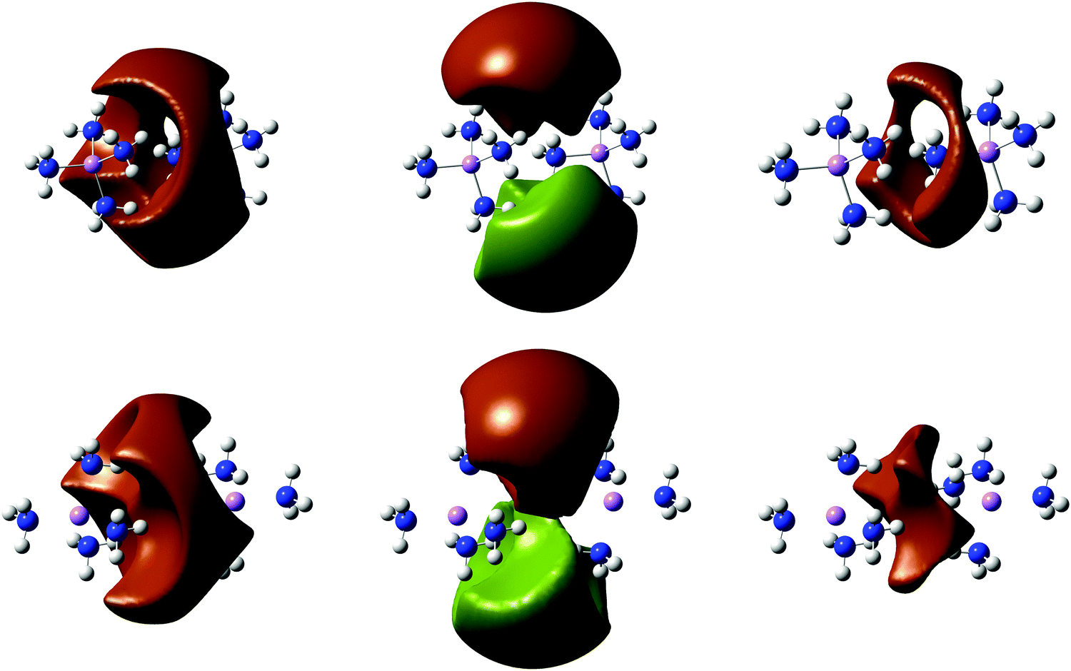
Fig. 11 shows EDR(r⃑;u_av) from RHF, UHF, and Brückner doubles calculations on solvated electron pairs. Table 3 shows the corresponding VDE and u_av. Fig. S15 (ESI†) shows the RHF and UHF frontier orbitals, and Fig. S16 (ESI†) shows the LSDA, B3LYP, and CCSD EDR(r⃑;u_av). Just as in Fig. 4 and 10, the RHF and UHF EDR(r⃑;u_av) highlight the same region of space as the RHF and UHF orbitals in Fig. S15 (ESI†). Both structures have a delocalized threefold symmetric RHF and BD EDR(r⃑;u_av), while the spin-up and spin-down UHF EDR(r⃑;u_av) show broken symmetry.

Table 3 Computed VDE and u_av for C_3v and D_3d (Li(NH₃)₄)₂ (Fig. 11)

Method	C 3v		D 3d
	VDE (eV)	u av (Angstrom)	VDE (eV)	u av (Angstrom)
RHF	7.13	7.2	7.09	7.0
UHF	7.38	5.5	7.28	5.6
LSDA	9.83	5.8	9.85	5.7
B3LYP	9.27	6.2	9.25	6.1
BHLYP	8.62	6.4	8.61	6.2
CCSD	8.30	6.3	8.26	6.2
BD	8.28	6.3	8.24	6.2

---

The most notable result in Table 3 is the dramatic role of nondynamical correlation. Ref. 4 argued that “the Li(NH₃)₄ SOMO is like a big hydrogen atom (or alkali metal) SOMO”. We find that (Li(NH₃)₄)₂ is like a stretched (“big”) H₂ with significant nondynamical correlation.⁵² Symmetry-broken UHF calculations stabilize the solvated electron pairs by 0.2–0.25 eV, and reduce their characteristic delocalization length u_av by almost 2 Angstrom. Symmetry-restricted CCSD, BD, and DFT calculations increase the VDE consistent with both dynamical and nondymaical correlation, and also significantly localize the electrons. The relatively large CCSD T1 diagnostic⁸⁴ 0.022 suggests that even these calculations may not capture all nondynamical correlation present. However, the results suffice to show how the EDR quantifies the localizing effects of nondynamical correlation.

D. Transition to a metallic state

We conclude by considering how the EDR gives insight into lithium–ammonia solutions' transition to a metallic state. Previous simulations suggest that solvated spin-paired electrons coalesce into tunnel-like extended states at 2–9 mole percent metal.^15–17 We simulate the coalescence of three such electron pairs confined in an extended (NH₃)₂₀ cavity (Fig. 12). The model system is small enough to permit accurate CASSCF calculations of “strong” nondynamical correlation. We emphasize that this model system does not capture all aspects of coalescence. For example, the six electrons are confined to the cavity by the localized basis set, the electron–NH₃ interactions are treated by a simple pseudopotential, and the cavity geometry is fixed at an artificial high-symmetry state. However, we suggest that this model suffices to illustrate the interplay of delocalization and nondynamical correlation.

Fig. 12 EDR(r⃑;u = 2.6 Angstrom) = 0.6 isosurfaces for RHF (top), LSDA (middle), and CASSCF (bottom) calculations on six electrons in an ammonia cavity.

Fig. 12 plots the EDR at u = 2.6 Angstrom from RHF, UHF, and CASSCF(6,12) calculations. This u value maximizes the RHF 〈EDR(u)〉, and is thus representative of the solvated electrons. Fig. 13 offers a complimentary perspective, showing EDR(x;u) for all delocalization lengths u, evaluated at points x along the cavity center and plotted using the conventions of Fig. 1. Fig. 13 also includes a UHF calculation on the heptet state of six unpaired electrons. Fig. S18 (ESI†) shows the corresponding electron densities.

Fig. 13 EDR(x;u) for multiple u values, plotted for points x along the center of the cavity in Fig. 12. Horizontal lines denote the u value plotted in Fig. 12.

The EDR in Fig. 12 and 13 illustrates the interplay of electron delocalization and correlation. The singlet RHF electrons form three electron pairs with limited inter-pair delocalization. The UHF heptet in Fig. 13 instead shows six nearly isolated electrons, shifted down to shorter delocalization lengths. CASSCF calculations on the singlet state show a mixture of these two effects. The CASSCF EDR shows a modest amount of inter-pair delocalization, consistent with the inter-pair interactions important to the transition to the metallic state.³⁶ The EDR also shifts down to lower delocalization lengths, consistent with the aforementioned correlation-induced localization. The CASSCF EDR is generally smaller (darker) than that from the RHF calculation, consistent with the normalization effects in Fig. 2. Finally, the LSDA captures the increased inter-pair interactions of CASSCF, but does not capture the detailed structure of the CASSCF state or the “full downward” shift to smaller delocalization lengths u.

IV. Conclusions

The results presented here illustrate that the electron delocalization range EDR(r⃑;u) is a useful theoretical tool for visualizing and quantifying the delocalization of solvated electrons. The density matrix plots in Fig. 1 illustrate how the EDR provides a specific, quantitative probe of the “off-diagonal” delocalization (coherence) critical to chemical bonding and reactivity. Fig. 6 illustrates that system-averaged u_av obtained from the EDR can reproduce existing MO-based measures of solvated electrons' average delocalization. Importantly, Fig. 4 shows that EDR(r⃑;u_av) directly links this system-averaged quantity back to a real-space picture. EDR(r⃑;u_av) highlights precisely the region of space containing the solvated electron, without requiring special selections or localization of orbitals. Such connections between system-averaged and real-space properties will help interpret the chemistry of more complicated systems. Finally, our studies of spin-paired electrons show that the density-matrix-based EDR is readily applicable to strongly correlated singlets systems where spin-density-based descriptors are unavailable (in the absence of symmetry breaking) and orbital-based descriptors can be qualitatively incorrect. To illustrate, Fig. S19 (ESI†) shows the natural orbital occupancies (MO-basis density matrix eigenvalues) from the CASSCF(6,12) calculations in Fig. 12 and 13. The first five natural orbitals have signficantly noininteger values, indicating a breakdown of the MO approximation. Overall, these results motivate continued application of the EDR to quantify and interpret the calculated electronic structures of delocalized and solvated electrons.

Acknowledgements

BGJ acknowledges support by the Department of Chemistry at Texas Christian University. The authors thank John M. Herbert for useful comments on the SOMO R_g of ref. 29.

References

1. B. Abel, U. Buck, A. L. Sobolewski and W. Domcke, Phys. Chem. Chem. Phys., 2012, 14, 22.
2. K. Maeda, M. T. J. Lodge, J. Harmer, J. H. Freed and P. P. Edwards, J. Am. Chem. Soc., 2012, 134, 9209.
3. W. Weyl, Ann. Phys., 1864, 121, 606.
4. E. Zurek, P. P. Edwards and R. Hoffmann, Angew. Chem., Int. Ed., 2009, 48, 8191.
5. M. T. J. H. Lodge, P. Cullen, N. H. Rees, N. Spencer, K. Maeda, J. R. Harmer, M. O. Jones and P. P. Edwards, J. Phys. Chem. B, 2013, 117, 13322.
6. L. Turi and P. Rossky, Chem. Rev., 2012, 112, 5641.
7. D.-F. Feng and L. Kevan, Chem. Rev., 1980, 80, 1.
8. L. Kevan, Acc. Chem. Res., 1981, 14, 138.
9. L. D. Jacobson and J. M. Herbert, Int. Rev. Phys. Chem., 2011, 30, 1.
10. J. R. Casey, A. Kahros and B. J. Schwartz, J. Phys. Chem. B, 2013, 117, 14173.
11. R. N. Barnett, U. Landman, C. L. Cleveland and J. Jortner, J. Chem. Phys., 1988, 88, 4421.
12. R. N. Barnett, U. Landman, C. L. Cleveland and J. Jortner, J. Chem. Phys., 1988, 88, 4429.
13. J. R. R. Verlet, A. E. Bragg, A. Kammrath, O. Cheshnovsky and D. M. Neumark, Science, 2005, 307, 93.
14. B. J. Schwartz and P. J. Rossky, J. Chem. Phys., 1994, 101, 6902.
15. Z. Deng, G. J. Martyna and M. L. Klein, Phys. Rev. Lett., 1992, 68, 2496.
16. Z. Deng, G. J. Martyna and M. L. Klein, Phys. Rev. Lett., 1993, 71, 267.
17. Z. Deng, G. J. Martyna and M. L. Klein, J. Phys. Chem., 1994, 100, 7590.
18. R. E. Larsen, W. J. Glover and B. J. Schwartz, Science, 2010, 329, 65.
19. J. M. Herbert and L. D. Jacobson, J. Phys. Chem. A, 2011, 115, 14470.
20. F. Uhlig, O. Marsalek and P. Jungwirth, J. Phys. Chem. Lett., 2012, 3, 3071.
21. I. A. Shkrob, J. Phys. Chem. A, 2006, 110, 3967.
22. T. Sommerfeld and K. M. Dreux, J. Chem. Phys., 2012, 137, 244302.
23. D. Ben-Amotz, J. Phys. Chem. Lett., 2011, 2, 1216.
24. R. S. Mulliken, J. Chem. Phys., 1955, 23, 1833.
25. Distinctions among, e.g., “core” and “valence” electrons are a colloquialism used here to aid understanding. All calculations treat electrons as indistinguishable Fermions.
26. F. Wang and K. D. Jordan, J. Chem. Phys., 2002, 116, 6973.
27. J. M. Herbert and M. Head-Gordon, J. Phys. Chem. A, 2005, 109, 5217.
28. J. M. Herbert and M. Head-Gordon, Phys. Chem. Chem. Phys., 2006, 8, 68.
29. C. F. Williams and J. M. Herbert, J. Phys. Chem. A, 2008, 112, 6171.
30. V. P. Vysotskiy, L. S. Cederbaum, T. Sommerfeld, V. K. Voora and K. D. Jordan, J. Chem. Theory Comput., 2012, 8, 893.
31. M. Gutowski, P. Skurski, A. I. Boldyrev, J. Simons and K. D. Jordan, Phys. Rev. Appl., 1996, 54, 1906.
32. M. Gutowski and P. Skurski, J. Chem. Phys., 1997, 107, 2968.
33. M. Gutowski, K. D. Jordan and P. Skurski, J. Phys. Chem. A, 1998, 102, 2624.
34. T. Sommerfeld, B. Bhattarai, V. P. Vysotskiy and L. S. Cederbaum, J. Chem. Phys., 2010, 133, 114301.
35. T. Sommerfeld, K. M. Dreux and R. Joshi, J. Phys. Chem. A, 2014, 118, 7320.
36. N. F. Mott, J. Phys. Chem., 1980, 84, 1199.
37. A. E. Reed, R. B. Weinstock and F. Weinhold, J. Chem. Phys., 1985, 83, 735.
38. K. B. Wiberg, C. M. Hadad, T. J. LePage, C. J. Breneman and M. J. Frisch, J. Phys. Chem., 1992, 96, 671.
39. P. Hohenberg and W. Kohn, Phys. Rev., 1964, 136, B864.
40. W. Kohn and L. Sham, Phys. Rev., 1965, 140, A1133.
41. F. Della Sala and A. Görling, J. Chem. Phys., 2001, 115, 5718.
42. F. Uhlig, J. M. Herbert, M. P. Coons and P. Jungwirth, J. Phys. Chem. A, 2014, 118, 7507.
43. R. F. W. Bader and M. E. Stephens, J. Am. Chem. Soc., 1975, 97, 7391.
44. R. W. F. Bader and G. L. Heard, J. Chem. Phys., 1999, 111, 8789.
45. A. D. Becke and K. E. Edgecombe, J. Chem. Phys., 1990, 92, 5397.
46. A. Savin, J. Mol. Struct., 2005, 727, 127.
47. T. Sommerfeld, J. Phys. Chem. A, 2008, 112, 11817.
48. T. Sommerfeld, A. DeFusco and K. D. Jordan, J. Phys. Chem. A, 2008, 112, 11021.
49. T. Sommerfeld, J. Chem. Theory Comput., 2013, 9, 4866.
50. B. G. Janesko, G. Scalmani and M. J. Frisch, J. Chem. Phys., 2014, 141, 144104.
51. E. R. Johnson, A. Otero-de-la Roza and S. G. Dale, J. Chem. Phys., 2013, 139, 184116.
52. O. Gunnarsson and B. I. Lundqvist, Phys. Rev. B: Condens. Matter Mater. Phys., 1976, 13, 4274.
53. D. Cremer, Mol. Phys., 2001, 99, 1899.
54. A. D. Becke, J. Chem. Phys., 2003, 119, 2972.
55. R. Ponec and D. L. Cooper, J. Phys. Chem. A, 2007, 111, 11294.
56. J. P. Perdew, A. Ruzsinszky, L. A. Constantin, J. Sun and G. I. Csonka, J. Chem. Theory Comput., 2009, 5, 902.
57. A. J. Cohen, P. Mori-Sánchez and W. Yang, J. Chem. Phys., 2008, 129, 121104.
58. M. J. Frisch, G. W. Trucks, H. B. Schlegel, G. E. Scuseria, M. A. Robb, J. R. Cheeseman, G. Scalmani, V. Barone, B. Mennucci, G. A. Petersson and H. Nakatsuji, et al., Gaussian Development Version, Revision H.35, Gaussian, Inc, Wallingford, CT, 2010.
59. A. Seidl, A. Görling, P. Vogl, J. A. Majewski and M. Levy, Phys. Rev. B: Condens. Matter Mater. Phys., 1996, 53, 3764.
60. G. E. Scuseria and H. F. Schaefer III, Chem. Phys. Lett., 1987, 142, 354.
61. N. C. Handy, J. A. Pople, M. Head-Gordon, K. Raghavachari and G. W. Trucks, Chem. Phys. Lett., 1989, 164, 185.
62. N. C. Handy and H. F. Schaefer III, J. Chem. Phys., 1984, 81, 5031.
63. S. H. Vosko, L. Wilk and M. Nusair, Can. J. Phys., 1980, 58, 1200.
64. A. D. Becke, Phys. Rev. Appl., 1988, 38, 3098.
65. C. Lee, W. Yang and R. G. Parr, Phys. Rev. B: Condens. Matter Mater. Phys., 1988, 37, 785.
66. A. D. Becke, J. Chem. Phys., 1993, 98, 5648.
67. P. J. Stephens, F. J. Devlin, C. F. Chabalowski and M. J. Frisch, J. Phys. Chem., 1994, 98, 11623.
68. A. D. Becke, J. Chem. Phys., 1993, 98, 1372.
69. O. A. Vydrov and G. E. Scuseria, J. Chem. Phys., 2006, 125, 234109.
70. B. G. Janesko, G. Scalmani and M. J. Frisch, J. Chem. Phys., 2014, 141, 034103.
71. R. E. Stratman, G. E. Scuseria and M. J. Frisch, Chem. Phys. Lett., 1996, 257, 213.
72. K. A. Peterson, J. Chem. Phys., 2003, 119, 11099.
73. K. Peterson and C. Puzzarini, Theor. Chem. Acc., 2005, 114, 283.
74. K. Hashimoto and K. Daigoku, Phys. Chem. Chem. Phys., 2009, 11, 9391.
75. J. J. P. Stewart, J. Mol. Model., 2007, 13, 1173.
76. R. A. Ogg Jr., Phys. Rev., 1946, 69, 668.
77. J. Jortner, J. Chem. Phys., 1959, 30, 839.
78. S. Tretiak and S. Mukamel, Chem. Rev., 2002, 102, 3171.
79. O. A. Vydrov, J. Heyd, A. V. Krukau and G. E. Scuseria, J. Chem. Phys., 2006, 125, 074106.
80. A. Khan, J. Chem. Phys., 2006, 125, 024307.
81. H. Thompson, J. C. Wasse, N. T. Skipper, S. Hayama, D. T. Bowron and A. K. Soper, J. Am. Chem. Soc., 2003, 125, 2572.
82. J. F. Stanton, J. Gauss and R. J. Bartlett, J. Chem. Phys., 1992, 97, 5554.
83. L. A. Barnes and R. Lindh, Chem. Phys. Lett., 1994, 223, 207.
84. T. J. Lee and P. R. Taylor, Int. J. Quantum Chem., 1989, 36, 199.

---

Footnote

† Electronic supplementary information (ESI) available. See DOI: 10.1039/c5cp01967b

---