Quantifying non-Markovianity for a chromophore–qubit pair in a super-Ohmic bath
Received
27th October 2014
, Accepted 16th February 2015
First published on 17th February 2015
Abstract
An approach based on a non-Markovian time-convolutionless polaron master equation is used to probe the quantum dynamics of a chromophore–qubit in a super-Ohmic bath. Utilizing a measure of non-Markovianity based on dynamical fixed points, we study the effects of the environmental temperature and the coupling strength on the non-Markovian behavior of the chromophore in a super-Ohmic bath. It is found that an increase in the temperature results in a reduction in the backflow information from the environment to the chromophore, and therefore, a suppression of non-Markovianity. In the weak coupling regime, increasing the coupling strength will enhance the non-Markovianity, while the effect is reversed in the strong coupling regime.
I. Introduction
Recent advances in spectroscopic techniques have allowed increasing deployment of nonlinear optical measurements to probe the dynamic properties of various condensed-matter and biological systems.1–16 An interesting example from two-dimensional electronic spectroscopy studies is the conjecture that long-lasting quantum coherence may exist in photosynthetic light harvesting systems.1–7 Nonlinear single molecule spectroscopic techniques, such as hole-burning and three-pulse photon echo spectroscopy,12 capable of generating truly homogeneous lineshapes by eliminating inhomogeneous broadening, have been used to probe chromophores embedded in organic glasses, revealing a wide range of spectral behaviors, where the coupling of chromophores to the surrounding medium (solvent, glass, host crystal, protein, etc.) may give rise to non-Markovian dynamics.
For low-temperature glasses and amorphous solids characterized by structural disorder, often only the two lowest energy levels of the double minimum potential need to be considered. Therefore, they can be modeled as a collection of two-level systems, and indeed such a model has been successfully employed to study their anomalous specific heat and thermal conductivity.17,18 With the local environment modeled as a collection of flipping qubits which modulate the chromophore transition frequency,19 Suárez and Silbey20 proposed a microscopic Hamiltonian to study the dynamics of a single chromophore in glasses, and demonstrated its correlation with the stochastic sudden jump model.21 Their dressed microscopic Hamiltonian is taken as our starting point to investigate the dynamics of a central chromophore embedded in a bath of qubits commonly found in low-temperature glasses.
In the aforementioned chromophore–qubit pair, the energy scales for the vibronic relaxation and spin-phonon coupling are comparable placing the system-bath interaction outside the usual weak coupling regime which is inaccessible to the traditional second-order perturbation methods.22–24 Therefore, non-perturbative approaches,25–31 including the numerically exact iterative path integral methods,29 sophisticated stochastic treatments of the system–bath models,30 and hierarchical equation of motion approach,31 have subsequently been proposed to treat such systems of intermediate coupling. However, these computationally intensive methods are inadequate for dealing with large systems or multiple-excitations. Recently, the non-Markovian time-convolutionless polaron master equation has been employed to describe the excitation dynamics in multichromophoric systems.24,32–36 The advantage of this master equation is that it is capable of depicting the dynamics in intermediate coupling regimes, handling initial non-equilibrium bath states, as well as spatially correlated environments. This method has been successfully applied to study the dynamics of two coupled pseudo-spins in contact with a dissipative bath and in addition, it was used to investigate the energy transfer of an extended spin-boson model by including an additional spin bath.36
Open quantum systems may exhibit interesting non-Markovian features that have been drawing sustained attention,37–40 and may be responsible for novel phenomena in chemical systems, such as dynamic control in polymers41 and transport enhancing in biosystems.42 More importantly, different degrees of non-Markovian behavior may bring about different physical phenomena. Thus, quantifying non-Markovian behavior will help gain a better understanding in the underlying systems. In addition, coherent control nowadays has been demonstrated over a large number of quantum systems of different complexity. A precise definition and quantification of the non-Markovianity brings this quantity into the context of coherent control, allowing researchers to consider it as a target variable. On-purpose manipulation of the non-Markovianity opens up fascinating perspectives on the optimization of energy and charge transport in open quantum systems by engineering their coupling to heat baths. Among various definitions of non-Markovianity that emerged,43–48 one of the earliest, widely-used definitions was proposed by Breuer, Laine and Piilo (BLP),43 which is based on the decreasing monotonicity of the trace distance under the completely positive and trace-preserving operations. One intuitive physical interpretation of this monotonicity is that the information of distinguishability always flows from the system to reservoir in a Markovian process. For non-Markovian dynamics, this monotonicity can be violated and the trace distance may increase during the dynamics, indicating that the information of distinguishability may flow back from the reservoir to the system.
In this paper, we propose a new measure of non-Markovianity based on the aforementioned mechanism for systems with dynamical fixed points. If N is the number of initial states one takes for numerical calculation, then this measure has a  numerical advantage compared with the BLP measure. By solving the time-convolutionless polaron master equation of the chromophore–qubit pair, we find fixed points for the chromophore dynamics. Utilizing the non-Markovianity measure based on the fixed points, we are allowed to quantify the non-Markovian behavior of the central chromophore. Furthermore, we analyze the effects of the temperature and the coupling between the chromophore and the qubit on the non-Markovianity, and it is found that the temperature can suppress the backflow of the information in our model. With respect to the effect of the chromophore–qubit coupling, the situation is more complicated with differing influences of the coupling on the non-Markovianity in different regimes. We will show that in the weak coupling regime, the increase of the coupling strength can enhance the non-Markovianity, while in the strong coupling regime, it will suppress the non-Markovianity. In addition, the non-Markovian behaviors of the chromophore–qubit pair and the corresponding quasi-particle after the polaron transformation are also investigated. It is found that the non-Markovian behavior vanishes after the polaron transformation due to the much reduced coupling between the dressed particle and the bath.
The paper is organized as follows. In Section II, we introduce the model and the time-convolutionless polaron master equation of the chromophore–qubit pair with additional discussion on the dynamical fixed points of the chromophore. In Section III, we revisit the BLP non-Markovianity measure and propose a new measure based on the dynamical fixed points of the system. In Section IV, we apply the new measure to our model and discuss the non-Markovian behavior of the chromophore. Section V draws the conclusion of this work.
II. Model and dynamics
Chromophore is a term that commonly refers to a certain moiety of a large organic molecule that gives rise to its optical absorption and fluorescence properties, such as the pi-conjugated double bonds between carbon atoms in carotenoids, or the chlorine-type macrocyclic ring complexed by magnesium in chlorophylls. In the context of our work, this term refers to an entire molecule when it is embedded in a host environment, such as a pigment molecule in crystalline (e.g., pentacene in p-terphenyl crystal) or amorphous materials (perylene in polyethylene). In either context, a chromophore can be simply modeled as a system with two electronic levels (the ground and the excited state) whose transition frequency can be modulated due to its interaction with the host environment.
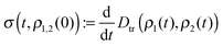
In this paper, we consider a two-level chromophore coupled to a phonon bath via a qubit, as shown in Fig. 1. A two-level system contains a quantum superposition of two independent (physically distinguishable) quantum states, which could refer to the qubit, spin, polarization, molecular transition and so on. A chromophore can be simply modeled as a system with two states whose transition frequency can be modulated due to its interaction with the host environment. In general, there can be more than two levels in the chromophore. However, non-Markovianity based on trace distance depicts the oscillating behavior of the trace distance between two evolved states. It does not directly reflect the oscillating information of populations in each level. Thus, the assumption of a two-level chromophore helps reveal the qualitative behavior of non-Markovianity. The Hamiltonian can be written as13,20,49
| | 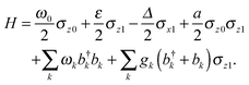 | (1) |
Here
σi0 :=
σi ⊗

and
σi1 :=

⊗
σi for
i =
x,
y,
z and
σi is a Pauli matrix. The subscript 0 (1) represents the subspaces of the chromophore (qubit). We have set
ℏ = 1 in this Hamiltonian.
ω0 and
ε are the transition frequencies.
Δ is the tunneling matrix element. The coupling strength between the chromophore and qubit is represented by the coefficient
a, which is related to the distance between the chromophore and qubit, as well as the spin orientation of the qubit.

is the Hamiltonian of the phonon bath, with

,
bk the creation and annihilation operators, respectively.
gk represents the coupling between the qubit and the reservoir. The Hamiltonian (
1) can be also obtained through a unitary transformation from a Hamiltonian in which the chromophore and the qubit are not directly coupled, but both interact with a common reservoir.
13,20
 |
| | Fig. 1 Schematics of the model. The chromophore interacts with the reservoir indirectly via a probe qubit. | |
To facilitate the dynamics calculation, we first perform a polaron transformation on the Hamiltonian (1). The generator of this transformation reads
where

. It is easy to verify the equality that exp(
U) = cosh(
B/2) +
σz1![[thin space (1/6-em)]](https://www.rsc.org/images/entities/char_2009.gif)
sinh(
B/2). After the polaron transformation, the new Hamiltonian can be written as
Here the effective quasi-particle Hamiltonian
![[H with combining tilde]](https://www.rsc.org/images/entities/i_char_0048_0303.gif) 0
0 has the form
| |  | (4) |
The bath Hamiltonian is unchanged as

and the effective interaction Hamiltonian
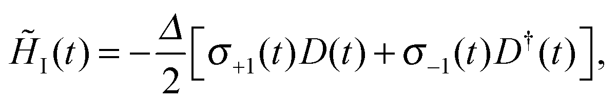
I can be expressed by
| |  | (5) |
where
Θ = 〈cosh
B〉 = 〈exp
B〉, and 〈·〉 denotes the thermal average. It is found that
| |  | (6) |
Given a bath spectral density

,
Θ can be rewritten as
| | 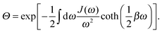 | (7) |
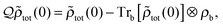
Throughout this paper, we consider the total initial state in the original basis as
| | | ρtot(0) = ρc ⊗ |0〉〈0|q ⊗ ρb, | (8) |
where
ρc is the reduced density matrix of the chromophore, |0〉〈0|
q denotes the spin “up” state of the qubit, and
ρb = exp(−
βHb)/
Z is the thermalized phonon state in the original representation before polaron transformation. Here
Z = Tr[exp(−
βHb)] is the partition function and
β = 1/(
kBT), with
T the temperature and
kB the Boltzmann constant. In the paper we set
kB = 1.
In the interaction picture, the time dependent interaction Hamiltonian can be expressed by I(t) = ei(0+Hb)tIe−i(0+Hb)t. After some algebra, we have
| |  | (9) |
in which the time dependent operator
σ±1(
t) reads
σ±1(
t) = e
i0tσ±1e
−i0t with
σ±1 = (
σx1 ±
iσy1)/2 being the effective raising (lowering) operator of the qubit. The reservoir correlated operator
D(
t) has the form
D(
t) = e
B(t) −
Θ, where
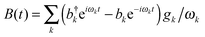
.
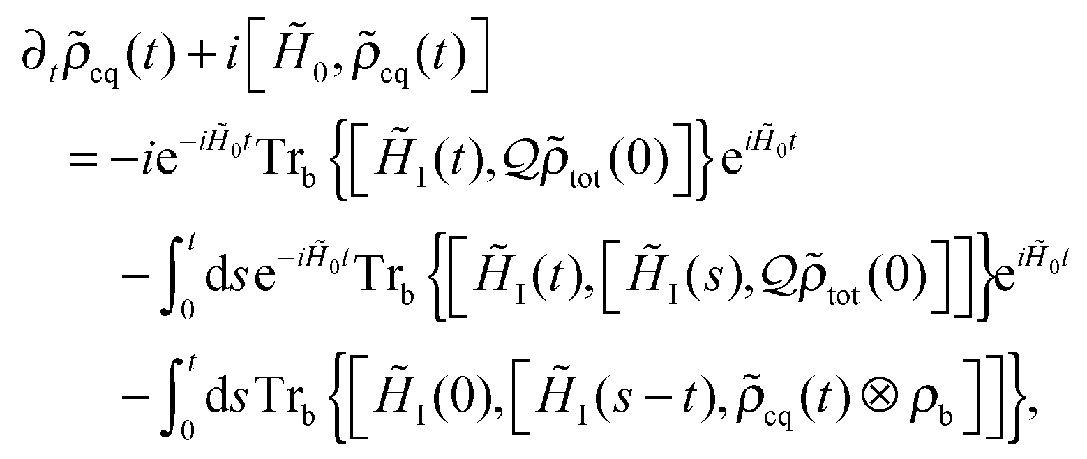
The time evolution of the quasi-particle described by the effective Hamiltonian (4) can be solved using the time-convolutionless polaron master equation.24,36,43 In the polaron representation, assuming that ![[small rho, Greek, tilde]](https://www.rsc.org/images/entities/i_char_e0e4.gif) cq is the reduced density matrix of the quasi-particle, the quantum master equation can be expressed by24,32,33,36
cq is the reduced density matrix of the quasi-particle, the quantum master equation can be expressed by24,32,33,36
| |  | (10) |
where
| |  | (11) |
with
tot(0) = e
Uρtot(0)e
−U being the density matrix of the total ensemble in the polaron representation. The general definition of the operator

is given by
50| | 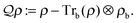 | (12) |
Taking into account the initial state (
8), one has
| | 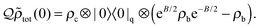 | (13) |
In this model, with respect to the chromophore dynamics, it is found that
ρc,fix = |0〉〈0|
c is a dynamical fixed point,
i.e., it does not evolve with the passage of time, for which we will give a short proof here. Taking |0〉〈0|
c as the initial state of the chromophore, in the Schrödinger picture, we have
| | | ρc(t) = Trqb(e−it|0〉〈0|c ⊗ |0〉〈0|q ⊗ ρbeit), | (14) |
where the trace is taken over the subspaces of the qubit and the environment. Based on the expression of
and the fact that |0〉 is the eigenstate of
σz = |0〉〈0| − |1〉〈1|, one finds that
| |0〉〈0|c ⊗ |0〉〈0|q ⊗ ρb = |0〉〈0|c ⊗ qb(|0〉〈0|q ⊗ ρb)qb, |
where
qb =
0qb +
I +
Hb, and
. It should be noted that though the notations in this Hamiltonian seem similar to those in
, the operators in
qb are actually confined to the subspace of the qubit and the environment. Then
eqn (14) can be rewritten as
ρc(
t) = |0〉〈0|
cTr
qb(e
−iqbt|0〉〈0|
q ⊗
ρbe
iqbt). Based on the cyclic permutation invariance of the trace, it can be simplified as
Thus, |0〉〈0|
c is a dynamical fixed point of the chromophore. More generally, it is known that diagonal fluctuations cause pure dephasing, while the off-diagonal fluctuations are responsible for population transfer. In our scenario, there are no off-diagonal fluctuations in the chromophore-related Hamiltonian. As a result, the decoherence of the chromophore is pure dephasing and all the diagonalized states are fixed points. Dynamical fixed points, which are especially useful in the study of the decoherence-free subspace, will be utilized in this work to construct a new measure of non-Markovianity.
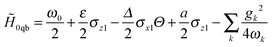
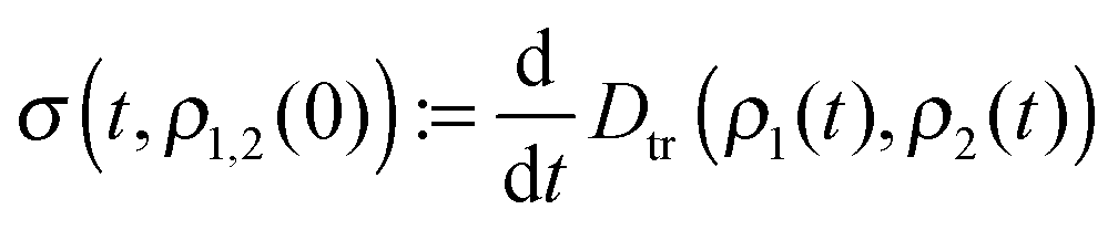
III. Non-Markovianity
To quantify the non-Markovian behavior, several measures have been proposed,43–48 among which the BLP measure43 relates the non-Markovian behavior to the backflow information from the reservoir to the system. The BLP definition is based on the trace distance| | | Dtr(ρ1,ρ2) := ½Tr|ρ1 − ρ2|, | (16) |
where  . For a single qubit, it is known that its density matrix can be expressed in the Bloch representation as
| | ρ = ½( + r·σ), + r·σ), | (17) |
where r is the Bloch vector, σ = (σx,σy,σz)T with σx,y,z the Pauli matrix, and  is the identity matrix. In this representation, the trace distance can be reduced to the Euclidean distance between the Bloch vectors51
| | | Dtr(ρ1,ρ2) = ½∥r1 − r2∥. | (18) |
Here ∥·∥ is the Euclidean distance. r1 and r2 are the corresponding Bloch vectors of ρ1 and ρ2, respectively.
The trace distance is monotonous when the system goes through the quantum channels, which can be described by the completely positive and trace-preserving maps. Physically, this monotonicity is explained intuitively by the fact that the information of distinguishability always flows from the system to the environment when the system goes through a quantum channel. Thus, the backflow of the information can be treated as non-Markovian behavior, or a memory effect in which the environment absorbs information from the system and returns some back to it, improving the distinguishability of the system. The BLP non-Markovianity is defined based on such a mechanism:
| |  | (19) |
where
| |  | (20) |
is the time derivative of the trace distance during the evolution. The maximum is taken over all pairs of initial states
ρ1(0) and
ρ2(0). According to the definition, it can be found that

. For a Markovian process, the non-Markovianity is zero,
i.e.,

.
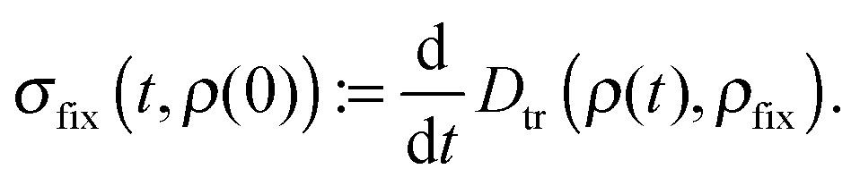
Dynamical fixed points may adopt various forms in physical systems, including states that are thermalized and ones within a decoherence-free subspace of a quantum system.52–55 An alternative definition of non-Markovianity is introduced below based on the trace distance in the presence of dynamical fixed points
| |  | (21) |
where
| |  | (22) |
Here
ρfix is the matrix for any dynamical fixed point, which satisfies the equation ∂
tρfix = 0, and the maximum is taken over all the initial states
ρ(0). It is easy to verify that

, and

for Markovian dynamics. The greater the value of

, the stronger is the non-Markovian behavior. However, the absolute value of non-Markovianity is in itself not meaningful as different dynamics or methods will show different amplitudes of oscillations.
Eqn (21) can be treated as a special form of the BLP measure as they both rely on the same mechanism,
i.e., monotonicity of the trace distance under the completely positive and trace-preserving maps. The value of

may be equal to or less than that of

. However, most of the physical information is contained in the variation of the non-Markovianity, not its absolute value. Therefore, despite

not containing as many pairs of initial states as

, it is still capable of describing the system behavior.
Moreover, compared with the BLP measure, the  measure has a numerical advantage. In principle, there are an infinite number of states in the Hilbert space. To carry out the numerical calculation of eqn (19), one has to sample a finite number of them. Assuming that this number is N, to take over all pairs of initial states, this generally requires N(N − 1)/2 times of calculations. Utilizing eqn (21), the calculation number is only N. Therefore, for some complex dynamics with fixed points, eqn (21) provides an efficient algorithm with a
  numerical advantage.
Since the maximization in  is not taken over all pairs of initial states in the Hilbert space, this measure does not capture the full information on non-Markovianity. This incompleteness of information on non-Markovianity is a trade-off of numerical advantage. However, since the non-Markovianity is a property of system dynamics, it should be independent of the initial states, in principle. As a matter of fact, dynamics can be called non-Markovian if the trace distance of any two states has increasing behavior during the evolution. Thus, the size of the set in which the maximization is performed is not a decisive factor on the issue of non-Markovianity. Admittedly, eqn (21) does not give a maximizing set as large as that of the BLP measure. We take a dynamical fixed point as the datum line because it does not evolve over the considered timescale. We then calculate the trace distance between this fixed point and all the states in the Hilbert space, indicating that the dynamical information of all initial states is involved in this measure. This explains why eqn (21) is capable of quantifying the behavior of non-Markovianity. Nevertheless, in some extreme mathematical cases where the numerical advantage of eqn (21) is not obvious, the BLP measure would be a better choice.
As we discussed in Section II, the state ρc,fix = |0〉〈0|c is a dynamical fixed point of the chromophore. Thus, it is convenient to use eqn (21) in our model to describe the non-Markovian behavior of the chromophore.
IV. Discussion
In this section, we will apply the non-Markovianity measure (21) in the model given in Section II. With this measure, we further discuss the non-Markovian behavior of the chromophore, as well as the chromophore–qubit pair, in the presence of the phonon bath. The effects of temperature and the coupling strength between the chromophore and qubit on the non-Markovianity will be discussed.
Generally, the expectation value of an observable A of the chromophore–qubit pair can be written as 〈A〉 = Trcqb[Aρtot(t)], where ρtot(t) is the total density matrix in the original representation including the chromophore, the qubit and the phonon bath. The subscripts c, q and b represent the subspaces of the chromophore, the qubit and the bath, respectively. Using the inverse polaron transformation and inserting  into the expression, one can obtain the expectation of A as24,36
| | | 〈A〉 = 〈A〉rel + 〈A〉irrel, | (23) |
where 〈
A〉
rel is the relevant part, which can be written as
| | | 〈A〉rel = Trcq[cq(t)Trb(eUAe−Uρb)], | (24) |
and the irrelevant part 〈
A〉
irrel reads
| |  | (25) |
When [
A,
U] = 0, the irrelevant part can be simplified into
. From the definition of

in
eqn (12), it is easy to see that

. Thus, for those observables that commute with the generator of the polaron transformation, their expectations contain only the relevant part,
i.e.,
| | | 〈A〉 = Trcq[Acq(t)]. | (26) |
A. The chromophore
With the above preliminary knowledge, we will try to reproduce the dynamical information of the chromophore in the original basis. For the chromophore–qubit pair, its density matrix in the original basis can always be decomposed into the form56,57| | ρcq = ¼( + rc·σ0 + rq·σ1 + m·σm) + rc·σ0 + rq·σ1 + m·σm) | (27) |
where rc and rq are the Bloch vectors of the chromophore and qubit, respectively, while σi = (σxi,σyi,σzi)T for i = 0, 1. and σm = (σx ⊗ σx,σy ⊗ σy,σz ⊗ σz)T. Through some straightforward calculations, one finds that| | | rc = (〈σx0〉, 〈σy0〉, 〈σz0〉)T, | (28) |
where the expectation 〈σi0〉 = Trcq(σi0ρcq) for i = x, y, z. As [σi0,U] = 0, based on eqn (26), the expectation of σi0 in the original representation is the same as that in the polaron representation, namely,| | | 〈σi0〉 = Trcq[σi0cq(t)]. | (29) |
In this way, we can reproduce the dynamical information of the chromophore. Using the expression of the Bloch vector rc, the trace distance between rc and the fixed point rc,fix can be written as| |  | (30) |
The equivalent expression using the elements of the density matrix is| |  | (31) |
Substituting this equation into eqn (21), the fixed-point non-Markovianity can be obtained as| |  | (32) |
with| |  | (33) |
Fig. 2 displays the time evolution of the trace distance of the chromophore. The initial states are chosen as rc1 = (1,0,0)T and rc,fix = (0,0,1)T. Here rc,fix is the Bloch vector of the dynamical fixed point of the chromophore: ρc,fix = |0〉〈0|c. The parameters are set as ε = ω0, Δ = 0.8ω0, a = 2ω0, and T = 0.5ω0. A super-Ohmic spectral density J(ω) = κωph−2ω3exp(−ω/ωc) is taken with the characteristic phonon frequency ωph = ω0, the cutoff frequency ωc = 4ω0 and the coupling strength κ = 0.1ω0. The red solid line in Fig. 2 is the result of the time-convolutionless master equation. As a comparison, we also display the corresponding dynamics of the trace distance from the Redfield equation. It is found from Fig. 2 that utilizing the time-convolutionless master equation, the trace distance has an oscillating component in its evolution, while it is monotonously decreasing using the Redfield theory. This monotonicity exists for any initial state, indicating vanishing non-Markovianity, which is in agreement with the fact that dynamics governed by the Redfield equation are Markovian. For the time-convolutionless master equation, the descending trend of the trace distance is due to the dissipative effect of the environment, indicating an information flow from the system to the environment. However, this information flow is by no means unidirectional. The oscillation of the trace distance demonstrates the backflow of information from the environment to the system, pointing to the non-Markovian behavior in the dynamics of the chromophore.
 |
| | Fig. 2 The dynamics of the trace distance of the chromophore. The red solid and blue dashed lines represent the results from the time-convolutionless master equation and the Redfield equation, respectively. The initial states are rc1 = (1,0,0)T and rc,fix = (0,0,1)T. The parameters are set as ε = ω0, Δ = 0.8ω0, a = 2ω0, and T = 0.5ω0. | |
As part of the system–environment correlation, the non-Markovianity must be affected by the temperature of the environment, as discussed in the literature.50,58,59 Here we also examine the influence of temperature on the non-Markovianity. Fig. 3 shows the behavior of non-Markovianity  as a function of temperature. The parameters in this figure are set as ε = ω0, Δ = 0.8ω0, and a = 4ω0. The spectral density and the relevant parameters are the same as those in Fig. 2. We have taken more than 1000 initial states for each temperature point in this plot. Fig. 3 demonstrates that an increase of temperature can suppress the non-Markovianity.
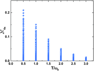 |
| | Fig. 3 The variation of non-Markovianity  as a function of the normalized temperature T/ω0. The parameters are set as ε = ω0, Δ = 0.8ω0, and a = 4ω0. The spectral density and the relevant parameters are the same as those in Fig. 2. as a function of the normalized temperature T/ω0. The parameters are set as ε = ω0, Δ = 0.8ω0, and a = 4ω0. The spectral density and the relevant parameters are the same as those in Fig. 2. | |
To further probe the temperature effect, we plot the evolution of the trace distance with specific initial states rc1 = (1,0,0)T and rc,fix = (0,0,1)T, as shown in Fig. 4. It is found that the increasing temperature can speed up the decay of the trace distance, as well as suppress its oscillation. More phonons are excited with the rise of temperature, leading to acceleration of the decoherence of the chromophore via the probe qubit. The acceleration of the decoherence will reduce the oscillation amplitudes of the coherence of the density matrix of the chromophore and increase its decay rate. Then, based on the equation Dtr2 = ρc,222(t) + |ρc,12(t)|2, one can see that the acceleration of decoherence results in a faster decay of the trace distance, and its oscillating amplitude, causing a further reduction of non-Markovianity and therefore a suppression of the information backflow.
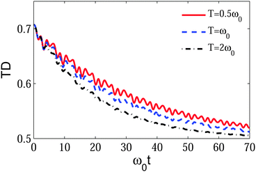 |
| | Fig. 4 Time evolution of the trace distance under different temperatures. The values of temperature T are 0.5ω0, ω0 and 2ω0 for the red solid line, the blue dashed line and black dashed dotted line, respectively. The parameters are set as ε = ω0, Δ = 0.8ω0, and a = 2ω0. The Bloch vectors of the initial states are rc1 = (1,0,0)T and rc,fix = (0,0,1)T. | |
The calculation of the BLP measure for the system studied in our manuscript requires a computation time that is inaccessible, making a direct comparison between the BLP non-Markovianity and the fixed-point non-Markovianity impossible. However, some of our results are in good agreement with a number of earlier studies50,58,59 of the BLP non-Markovianity that show a suppressed behavior with an increasing temperature. The fixed-point non-Markovianity is thus a compromised form of the BLP measure and is qualified to capture the non-Markovian behavior of dynamics in this system.
Another important parameter affecting the system–environment correlation is the coupling strength a between the chromophore and qubit, which is proportional to the angular orientation parameter η of the dipole–dipole interaction and inversely proportional to the cube of the distance r between the chromophore and qubit,13i.e., a ∝ η/r3. In previous studies where the dynamical processes are solved by perturbation methods, it is difficult to gauge the effect of the coupling strength on non-Markovianity due to the weak coupling constraint. In our case, this constraint is reflected by the parameter κ in the spectral density, i.e., κ cannot be arbitrarily large. However, the coupling between the chromophore and qubit can be chosen in a wide range, without affecting the accuracy of the time-convolutionless master equation, allowing a study on the non-Markovianity in the strong coupling regime.
Fig. 5 shows the variation of the non-Markovianity  as a function of coupling parameter a. Other parameters in this figure are set as ε = ω0, Δ = 0.8ω0, and T = 0.5ω0. The spectral density and the relevant parameters are the same as those in the previous figures. Similar to Fig. 3, we also take more than 1000 initial states for each value of a. When a = 0, the non-Markovianity vanishes. This is because when the chromophore is isolated, its evolution turns out to be unitary and the trace distance is unchanged for a unitary transformation. In other words, there is no information exchange between the chromophore and qubit in this case. In the weak coupling regime, an increase of a can enhance the non-Markovianity. This enhancement effect is well known in the community and is one of the main reasons why the Markovian approximation is applicative in the weak coupling regime. However, when a is large, the effect is totally contrary. In this regime, an increase of a will suppress the non-Markovianity. In our case, the maximum non-Markovianity is obtained around a = ω0, a value that may change if system parameters vary.
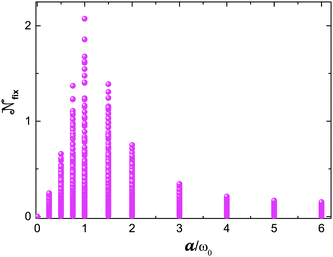 |
| | Fig. 5 The variation of non-Markovianity  as a function of the normalized coupling strength a/ω0. The parameters in this figure are set as ε = ω0, Δ = 0.8ω0, and T = 0.5ω0. The spectral density and the relevant parameters are the same as those in Fig. 2. as a function of the normalized coupling strength a/ω0. The parameters in this figure are set as ε = ω0, Δ = 0.8ω0, and T = 0.5ω0. The spectral density and the relevant parameters are the same as those in Fig. 2. | |
To obtain a deeper understanding of how the system–bath coupling suppresses the non-Markovianity in the strong coupling regime, we plot the time evolution of the trace distances for three values of a in Fig. 6. The red solid line, the black dashed dotted line and the blue dashed line represent the trace distances with a = 2ω0, a = 3ω0 and a = 6ω0, respectively. Other parameters are the same as those in Fig. 5. The black and blue lines are shifted downward in the right panel to better distinguish the curves. It is found that an increase of coupling strength will not affect the decay rate of the trace distance, but does affect its oscillation amplitude. This is because in this coupling regime, the behavior of the system trends to a way similar to the overdamped behavior. The oscillation of the off-diagonal element of the density matrix is suppressed.
 |
| | Fig. 6 The time evolution of the trace distance with three values of the coupling strength a. Left panel: the red solid line, the black dashed dotted line and the blue dashed line represent the trace distances with a = 2ω0, a = 3ω0 and a = 6ω0, respectively. Other parameters are the same as in Fig. 5. Right panel: the solid red (dashed blue) lines in the left panel are shifted upward (downward) to better distinguish the three cases. | |
To show this, we plot as a function of time the square norm of the off-diagonal element of the chromophore's reduced density matrix in Fig. 7. Two specific initial states, labeled 1 and 2, are considered: ρ1,11 = 0.5, ρ1,12 = 0.2 and ρ2,11 = 0.7, ρ2,12 = 0.4. The solid (dashed) blue and red lines represent |ρ1,12|2(|ρ2,12|2) for a = 2ω0 and a = 4ω0, respectively. Other parameters are the same as in Fig. 5. It is shown in Fig. 7 that the oscillation amplitude of the off-diagonal elements decreases with increasing a, but the decay rate stays constant. As this oscillation attenuation happens to all states but the fixed points in the Hilbert space, any measure based on the trace distance will exhibit this behavior, including the BLP measure. It is thus an intrinsic property of the non-Markovian system.
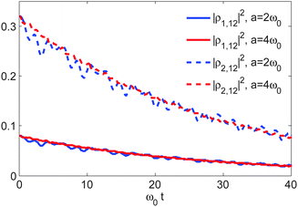 |
| | Fig. 7 Time evolution of the square norm of the off-diagonal element of chromophore's reduced density matrix. Two initial states, labeled 1 and 2, are considered: ρ1,11 = 0.5, ρ1,12 = 0.2 and ρ2,11 = 0.7, ρ2,12 = 0.4. The solid (dashed) blue and red lines represent |ρ1,12|2 (|ρ2,12|2) for a = 2ω0 and a = 4ω0, respectively. Other parameters are the same as in Fig. 5. | |
Systems of coupled chromophores are very relevant for many physical phenomena in physical chemistry. The only requirement of eqn (21) is the existence of dynamical fixed points, which is very common when the systems only have diagonal fluctuations. This implies that the present work on a single chromophore can be easily extended to treat multi-chromophore systems.
B. The chromophore–qubit pair
In this subsection, we look into the non-Markovian behavior of the chromophore–qubit pair in the presence of the bath. First, its dynamics can be obtained by calculating the vectors rc, rq and m in eqn (27). The expression of rc has been given in the previous subsection. Now we will focus on rq and m. Based on eqn (27), one can easily find that| | | rq = (〈σx1〉, 〈σy1〉, 〈σz1〉)T, | (34) |
| | | m = (〈σx ⊗ σx〉, 〈σy ⊗ σy〉, 〈σz ⊗ σz〉)T. | (35) |
As some of the operators above do not commute with the generator U, the corresponding irrelevant parts of the expectations do not vanish. In general, this irrelevant contribution is hard to obtain because of the complex form of  . For simplicity, one can choose the zeroth order of
  as an approximation.24,36 In ref. 24, the zeroth order approximation was taken in the Schrödinger picture, i.e.,
| 〈A〉Sirrel = Trcq[Aρcq(0)] − Trcq[cq(0)Trb(eUAe−Uρb)], |
while the approximation can also be made in the interaction picture,
where tot,I is the density matrix of the total ensemble in the interaction picture. When [A,U] = 0, the irrelevant part vanishes, then the two approximations are actually the same.
Since the density matrix in the original basis is our main concern, we calculate the differences of the expectations 〈σi1〉 and 〈σi ⊗ σi 〉 for i = x, y by performing these two approximations. Through some straightforward calculation, it can be found that the irrelevant part 〈σx1〉Iirrel = 2Re[χ(t)〈σ+1(t)〉ρcq(0)], where the time-dependent function χ(t) is defined as  , Re(·) denotes the real part, and 〈·〉ρcq(0) := Trcq[·ρcq(0)]. Here ρcq(0) = ρc ⊗ |0〉〈0|q. Similarly, one can obtain that 〈σy1〉Iirrel = 2Im[χ(t)〈σ+1(t)〉ρcq(0)]. As the polaron transformation generator U has nothing to do with the subspace of the chromophore, one arrives at 〈σx ⊗ σx〉Iirrel = 2Re[χ(t)〈{σx ⊗ σ+}(t)〉ρcq(0)], where {σx ⊗ σ+}(t) := ei0t(σx ⊗ σ+)e−i0t is the time dependent operator of σx ⊗ σ+ in the interaction picture. It is therefore found that 〈σy ⊗ σy〉Iirrel = 2Im[χ(t)〈{σy ⊗ σ+}(t)〉ρcq(0)]. Utilizing the approximation in the Schrödinger picture, and considering the initial state (8), the irrelevant parts of the expectations of these four operators all vanish. We will compare below the expectation values from these two approximations.
Denote Γi = 〈σi1〉Sirrel − 〈σi1〉Iirrel and Γii = 〈σi ⊗ σi〉Sirrel − 〈σi ⊗ σi〉Iirrel, where i = x, y, as the differences in operator expectation values between the two approximations. In Fig. 8, Γi and Γii are plotted as a function of time, where the parameters are set as ε = ω0, Δ = 0.8ω0, T = 0.5ω0, and a = 4ω0. The spectral density and the relevant parameters are the same as those in Fig. 2. The initial Bloch vector for the chromophore is taken as rc1 = (1,0,0)T. The blue solid, black dashed dotted, red dashed and pink dotted lines represent Γx, Γy, Γxx and Γyy, respectively. It is found that the differences in the expectation values are small and short-lived, disappearing beyond ω0t = 2. For convenience, the approximation performed in the Schrödinger picture is chosen because the irrelevant part of the expectation values we are interested in always vanish in this case.
 |
| | Fig. 8 The variations of Γi and Γii for i = x, y as a function of time. Here Γi = 〈σi1〉Sirrel − 〈σi1〉Iirrel and Γii = 〈σi ⊗ σi〉Sirrel − 〈σi ⊗ σi〉Iirrel. The parameters in this figure are set as ε = ω0, Δ = 0.8ω0, T = 0.5ω0, and a = 4ω0. The spectral density and the relevant parameters are the same as those in Fig. 2. The blue solid, black dashed dotted, red dashed and pink dotted lines represent Γx, Γy, Γxx and Γyy, respectively. | |
Thus, for the zeroth order approximation, taking into account the initial state (eqn (8)), the expectation value of operator A has the form
| | | 〈A〉 = Trcq[cq(t)Trb(eUAe−Uρb)]. | (36) |
Here
A =
σx1,
σy1,
σx ⊗
σx, or
σy ⊗
σy. Density matrix dynamics can be obtained for the chromophore–qubit pair in the original basis. Keeping in mind the fact that e
Uσx1e
−U =
σx1cosh
B +
iσy1sinh
B, and 〈sinh
B〉 = 0, and utilizing the zeroth approximation, the expectation value of
σx1 in the original basis can be written as 〈
σx1〉 =
ΘTr
eq[
σx1cq(
t)]. Similarly, one can obtain that 〈
σy1〉 =
ΘTr
eq[
σy1cq(
t)] and 〈
σi ⊗
σi〉 =
ΘTr
eq[
σi ⊗
σicq(
t)] for
i =
x,
y. Moreover, based on
eqn (26), we have 〈
σz1〉 = Tr
eq[
σz1cq(
t)] and 〈
σz ⊗
σz 〉 = Tr
eq[
σz ⊗
σzcq(
t)]. Finally, one can obtain the density matrix of the chromophore–qubit pair in the original basis under the zeroth order approximation as
| | | ρcq(t) = MΘ·cq(t), | (37) |
where · denotes the Hadamard product and
| |  | (38) |
Now we are in a position to study the non-Markovian behavior of the chromophore–qubit pair before the polaron transformation and that of the phonon-dressed quasi-particle.
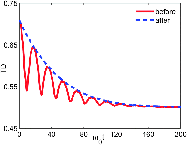
Fig. 9 shows the time evolution of the trace distances of the density matrices for the chromophore–qubit pair and the quasi-particle. The parameters in this plot are set as
ε =
ω0,
Δ = 0.8
ω0, and
a =
ω0. The initial states of the chromophore–qubit pair are chosen as
ρc,half ⊗ |0〉〈0|
q and |0〉〈0|
c ⊗ |0〉〈0|
q. Here
ρc,half reads
| |  | (39) |
 |
| | Fig. 9 Time evolution of the trace distance for the chromophore–qubit pair. The parameters are set as ε = ω0, Δ = 0.8ω0, and a = ω0. The spectral density is chosen as the same as that chosen before. The red solid line represents the trace distance before the polaron transformation and the blue dashed line represents that after the transformation. | |
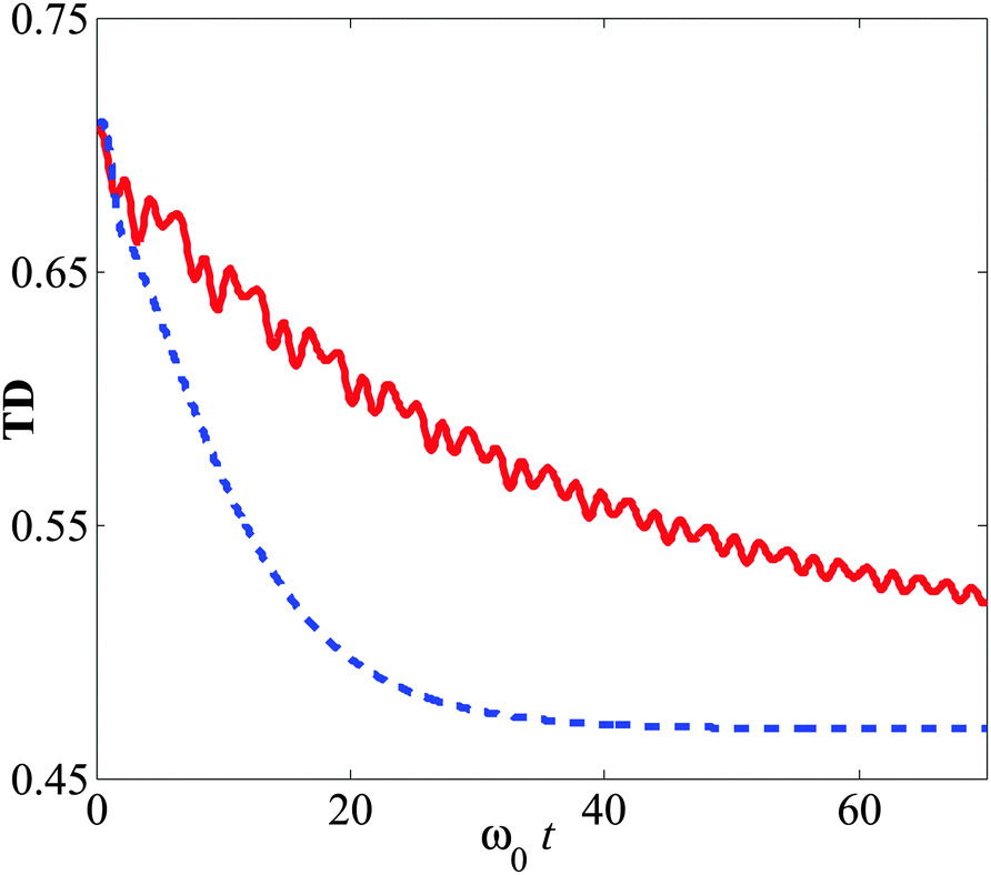
After the polaron transformation, the initial states of the quasi-particle take the same form. In Fig. 9, the solid and dashed lines depict the trace distance of the density matrices before and after the polaron transformation, respectively, and it is clear that before the polaron transformation, there are oscillations in the trace-distance dynamics implying non-Markovian behavior, while after the polaron transformation the trace distance monotonously decreases with the passage of time, an observation in agreement with the well-known fact that the polaron transformation reduces the effective interaction between the quasi-particle and the bath.
V. Conclusion
In conclusion, utilizing a non-Markovian time-convolutionless polaron master equation we probe the dynamics of a central chromophore interacting with a phonon reservoir via a probe qubit. An in-depth analysis is carried out on the non-Markovian behavior of the dynamics, for which a measure of non-Markovianity is provided based on dynamical fixed points of the system. This measure of non-Markovianity is analogous to the BLP measure but has a  numerical advantage.
Using this measure, we have discussed the effects of the bath temperature and the strength of the chromophore–qubit coupling on the non-Markovian behavior of the chromophore. It is found that an increase in the temperature brings about a reduction in the non-Markovianity. In the weak coupling regime, an increase in the coupling is found to enhance the non-Markovianity, while in the strong coupling regime, it suppresses the non-Markovianity. The non-Markovianity maximum is found in the near resonance regime (around a = ω0) for T = 0.5ω0, a value that may be sensitive to other system parameters such as the temperature and the spectral density of the bath. In addition, we compare the non-Markovian behavior of the chromophore–qubit combination before and after the polaron transformation. It is found that the non-Markovian behavior vanishes after the polaron transformation.
Non-Markovianity is of great interest in a variety of topics, such as steady-state entanglement maintenance,60 quantum teleportation,61 and precision estimation under noise in quantum metrology.62 Thus, finding optimal conditions to maximize non-Markovianity is useful for many situations. It is our hope that this work may inspire future experimental and theoretical endeavor to quantify non-Markovianity in relevant fields.
Acknowledgements
The authors thank Maxim Gerlin, Jian Ma, and Lipeng Chen for useful discussions. One of us (JL) is especially indebted to Xiao-Ming Lu for many valuable suggestions. This work was supported by the Singapore National Research Foundation through the Competitive Research Programme (CRP) under the Project No. NRF-CRP5-2009-04. One of us (XW) also acknowledges support from NFRPC through Grant No. 2012CB921602 and from NSFC through Grant No. 11475146.
References
- G. S. Engel, T. R. Calhoun, E. L. Read, T.-K. Ahn, T. Mancal, Y.-C. Cheng, R. E. Blankenship and G. R. Fleming, Nature, 2007, 446, 782–786 CrossRef CAS PubMed.
- H. Lee, Y.-C. Cheng and G. R. Fleming, Science, 2007, 316, 1462 CrossRef CAS PubMed.
- E. Collini, C. Y. Wong, K. E. Wilk, P. M. G. Curmi, P. Brumer and G. D. Scholes, Nature, 2010, 463, 644 CrossRef CAS PubMed.
- G. Panitchayangkoon, D. Hayes, K. A. Fransted, J. R. Caram, E. Harel, J. Wen, R. E. Blankenship and G. S. Engel, Proc. Natl. Acad. Sci. U. S. A., 2010, 107, 12766 CrossRef CAS PubMed.
- M. Sarovar, A. Ishizaki, G. R. Fleming and K. B. Whaley, Nat. Phys., 2010, 6, 462–467 CrossRef CAS.
- A. Ishizaki, T. R. Calhoun, G. S. Schlau-Cohen and G. R. Fleming, Phys. Chem. Chem. Phys., 2010, 12, 7319–7337 RSC.
- L. A. Pachón and P. Brumer, Phys. Chem. Chem. Phys., 2012, 14, 10094–10108 RSC.
- A. G. Dijkstra and Y. Tanimura, Phys. Rev. Lett., 2010, 104, 250401 CrossRef.
- B. Kozankiewicz,
et al.
, J. Chem. Phys., 1994, 101, 9337 CrossRef CAS PubMed; A. M. Stoneham, Rev. Mod. Phys., 1969, 41, 82 CrossRef; H. C. Meijers,
et al.
, Phys. Rev. Lett., 1992, 68, 381 CrossRef.
- Y. Zhao,
et al.
, Phys. Rev. B, 2004, 70, 195113 CrossRef; Y. Y. Zhang,
et al.
, Phys. Rev. B, 2010, 81, 121105 CrossRef; Y. Y. Zhang,
et al.
, J. Chem. Phys., 2012, 137, 034108 CrossRef PubMed.
- H. M. Sevian,
et al.
, J. Chem. Phys., 1992, 97, 8 CrossRef CAS PubMed; P. Shenai,
et al.
, J. Phys. Chem. A, 2013, 117, 12320 CrossRef PubMed.
- Y. S. Bai,
et al.
, Phys. Rev. B, 1989, 39, 11066 CrossRef CAS; K.-A. Littau,
et al.
, J. Chem. Phys., 1990, 92, 4145 CrossRef PubMed; H. C. Meijers,
et al.
, Phys. Rev. Lett., 1992, 68, 381 CrossRef; R. Wannemacher,
et al.
, Chem. Phys. Lett., 1993, 206, 1 CrossRef.
- F. Brown and R. Silbey, J. Chem. Phys., 1998, 108, 7434–7450 CrossRef CAS PubMed.
- P. D. Reilly,
et al.
, J. Chem. Phys., 1994, 101, 959 CrossRef CAS PubMed; P. D. Reilly,
et al.
, J. Chem. Phys., 1994, 101, 965 CrossRef PubMed; P. D. Reilly,
et al.
, Phys. Rev. Lett., 1993, 71, 425 CrossRef.
- B. Luo, J. Ye, C. Guan and Y. Zhao, Phys. Chem. Chem. Phys., 2010, 12, 15073–15084 RSC.
- A. de la Lande, N. S. Babcock, J. Rezac, B. Levy, B. C. Sanders and D. R. Salahub, Phys. Chem. Chem. Phys., 2012, 14, 5902–5918 RSC.
- R. C. Zeller,
et al.
, Phys. Rev. B, 1971, 4, 2029 CrossRef CAS; J. L. Black,
et al.
, Phys. Rev. B, 1977, 16, 2879 CrossRef.
- A. Heuer and R. J. Silbey, Phys. Rev. B, 1994, 49, 1441 CrossRef CAS; A. Heuer and R. J. Silbey, Phys. Rev. B, 1993, 48, 9411 CrossRef; A. Heuer and R. J. Silbey, Phys. Rev. Lett., 1993, 70, 3911 CrossRef.
- W. A. Phillips, J. Low Temp. Phys., 1972, 7, 351 CrossRef CAS; P. W. Anderson, B. I. Haiperin and C. M. Varma, Philos. Mag., 1972, 25, 1 CrossRef.
- A. Suárez and R. Silbey, J. Phys. Chem., 1994, 98, 7329–7336 CrossRef; A. Suárez and R. Silbey, Chem. Phys. Lett., 1994, 218, 445–453 CrossRef.
- J. R. Klauder and P. W. Anderson, Phys. Rev., 1962, 125, 912 CrossRef CAS.
- S. Jang, J. Chem. Phys., 2009, 131, 164101 CrossRef PubMed; S. Jang, J. Chem. Phys., 2011, 135, 034105 CrossRef PubMed.
- Y. C. Cheng and G. R. Fleming, Annu. Rev. Phys. Chem., 2009, 60, 241 CrossRef CAS PubMed.
- A. Kolli, A. Nazir and A. Olaya-Castro, J. Chem. Phys., 2011, 135, 154112 CrossRef PubMed.
- K. H. Hughes, C. D. Christ and I. Burghardt, J. Chem. Phys., 2009, 131, 124108 CrossRef PubMed.
- J. Prior, A. W. Chin, S. F. Huelga and M. B. Plenio, Phys. Rev. Lett., 2010, 105, 050404 CrossRef.
- M. Thorwart, J. Eckel, J. H. Reina, P. Nalbach and S. Weiss, Chem. Phys. Lett., 2009, 478, 234 CrossRef CAS PubMed.
- P. Nalbach, J. Eckel and M. Thorwart, New J. Phys., 2010, 12, 065043 CrossRef.
- M. M. Sahrapour,
et al.
, J. Chem. Phys., 2013, 138, 114109 CrossRef CAS PubMed; N. Makri,
et al.
, J. Chem. Phys., 1995, 102, 4600 CrossRef PubMed; N. Makri,
et al.
, J. Chem. Phys., 1995, 102, 4611 CrossRef PubMed; E. R. Dunkel,
et al.
, J. Chem. Phys., 2008, 129, 114106 CrossRef PubMed; P. Huo,
et al.
, J. Chem. Phys., 2010, 133, 184108 CrossRef PubMed; P. Huo,
et al.
, J. Chem. Phys., 2012, 136, 115102 CrossRef PubMed.
- J. Roden, A. Eisfeld, W. Wolff and W. T. Strunz, Phys. Rev. Lett., 2009, 103, 058301 CrossRef.
- A. Ishizaki,
et al.
, J. Chem. Phys., 2009, 130, 234110 CrossRef CAS PubMed; A. Ishizaki,
et al.
, Proc. Natl. Acad. Sci. U. S. A., 2009, 106, 17255 CrossRef PubMed; M. Tanaka,
et al.
, J. Chem. Phys., 2010, 132, 214502 CrossRef PubMed; A. Sakurai,
et al.
, J. Phys. Chem. A, 2011, 115, 4009–4022 CrossRef PubMed.
- S. Jang, Y. C. Cheng, D. R. Reichman and J. D. Eaves, J. Chem. Phys., 2008, 129, 101104 CrossRef PubMed.
- S. Jang, J. Chem. Phys., 2009, 131, 164101 CrossRef PubMed.
- A. Nazir, Phys. Rev. Lett., 2009, 103, 146404 CrossRef.
- D. P. S. McCutcheon and A. Nazir, Phys. Rev. B, 2011, 83, 165101 CrossRef.
- N. Wu and Y. Zhao, J. Chem. Phys., 2013, 139, 054118 CrossRef CAS PubMed; K. W. Sun and Y. Zhao, J. Phys. Chem. A, 2014, 118, 2220 CrossRef PubMed.
- M. M. Wolf,
et al.
, Phys. Rev. Lett., 2008, 101, 150402 CrossRef CAS; E.-M. Laine,
et al.
, Phys. Rev. A, 2010, 81, 062115 CrossRef; E.-M. Laine,
et al.
, Sci. Rep., 2014, 4, 4620 Search PubMed; J. Cerrillo and J. Cao, Phys. Rev. Lett., 2014, 112, 110401 CrossRef.
- M. J. W. Hall,
et al.
, Phys. Rev. A, 2014, 89, 042120 CrossRef CAS; F. F. Fanchini,
et al.
, Phys. Rev. A, 2013, 88, 012105 CrossRef; H.-B. Chen,
et al.
, Phys. Rev. E, 2014, 89, 042147 CrossRef; C. A. Mujica-Martinez,
et al.
, Phys. Rev. E, 2013, 88, 062719 CrossRef; F. F. Fanchini,
et al.
, Phys. Rev. Lett., 2014, 112, 210402 CrossRef.
- Á. Rivas, S. F. Huelga and M. B. Plenio, Rep. Prog. Phys., 2014, 77, 094001 CrossRef PubMed.
- B.-H. Liu, L. Li, Y.-F. Huang, C.-F. Li, G.-C. Guo, E.-M. Laine, H.-P. Breuer and J. Piilo, Nat. Phys., 2011, 7, 931 CrossRef CAS.
- T. Guérin, O. Bénichou and R. Voituriez, Nat. Chem., 2012, 4, 568–573 CrossRef PubMed.
- P. Rebentrost, R. Chakraborty and A. Aspuru-Guzik, J. Chem. Phys., 2009, 131, 184102 CrossRef PubMed.
- H.-P. Breuer, E.-M. Laine and J. Piilo, Phys. Rev. Lett., 2009, 103, 210401 CrossRef.
- Á. Rivas, S. F. Huelga and M. B. Plenio, Phys. Rev. Lett., 2010, 105, 050403 CrossRef.
- J. Liu, X.-M. Lu and X. Wang, Phys. Rev. A, 2013, 87, 042103 CrossRef.
- X.-M. Lu, X. Wang and C. P. Sun, Phys. Rev. A, 2010, 82, 042103 CrossRef; S. C. Hou, X. X. Yi, S. X. Yu and C. H. Oh, Phys. Rev. A, 2011, 83, 062115 CrossRef.
- S. Luo, S. Fu and H. Song, Phys. Rev. A, 2012, 86, 044101 CrossRef.
- D. Chrusćinśki and A. Kossakowski, Phys. Rev. Lett., 2010, 104, 070406 CrossRef; D. Chruściński and S. Maniscalco, Phys. Rev. Lett., 2014, 112, 120404 CrossRef.
- Q. H. Chen, Y. Y. Zhang, T. Liu and K. L. Wang, Phys. Rev. A, 2008, 78, 051801 CrossRef.
-
H.-P. Breuer and F. Petruccione, The Theory of Open Quantum Systems, Oxford University Press, New York, 2002 Search PubMed.
-
M. A. Nielsen and I. L. Chuang, Quantum Computation and Quantum Information, Cambridge University Press, Cambridge, 2000 Search PubMed.
-
D. A. Lidar and K. B. Whaley, in Irreversible Quantum Dynamics, Lecture Notes in Physics, ed. F. Benatti and R. Floreanini, Springer, Berlin, 2003, vol. 622, pp. 83–120, and the references therein Search PubMed.
- L.-M. Duan and G.-C. Guo, Phys. Rev. Lett., 1997, 79, 1953 CrossRef CAS.
- P. Zanardi and M. Rasetti, Phys. Rev. Lett., 1997, 79, 3306 CrossRef CAS.
- H.-N. Xiong, W.-M. Zhang, M. W.-Y. Tu and D. Braun, Phys. Rev. A, 2012, 86, 032107 CrossRef.
- U. Fano, Rev. Mod. Phys., 1983, 55, 855 CrossRef CAS.
- S. Luo, Phys. Rev. A, 2008, 77, 042303 CrossRef.
- G. Clos and H.-P. Breuer, Phys. Rev. A, 2012, 86, 012115 CrossRef.
- R. Vasile, F. Galve and R. Zambrini, Phys. Rev. A, 2014, 89, 022109 CrossRef.
- S. F. Huelga, Á. Rivas and M. B. Plenio, Phys. Rev. Lett., 2012, 108, 160402 CrossRef.
-
B. Bylicka, D. Chruściński, S. Maniscalco, E-print: arXiv: 1301.2585.
- A. W. Chin, S. F. Huelga and M. B. Plenio, Phys. Rev. Lett., 2012, 109, 233601 CrossRef CAS; B. M. Escher, R. L. de Matos Filho and L. Davidovich, Nat. Phys., 2011, 7, 406–411 CrossRef.
|
| This journal is © the Owner Societies 2015 |
Click here to see how this site uses Cookies. View our privacy policy here. 
 Open Access Article
 This Open Access Article is licensed under a
  numerical advantage compared with the BLP measure. By solving the time-convolutionless polaron master equation of the chromophore–qubit pair, we find fixed points for the chromophore dynamics. Utilizing the non-Markovianity measure based on the fixed points, we are allowed to quantify the non-Markovian behavior of the central chromophore. Furthermore, we analyze the effects of the temperature and the coupling between the chromophore and the qubit on the non-Markovianity, and it is found that the temperature can suppress the backflow of the information in our model. With respect to the effect of the chromophore–qubit coupling, the situation is more complicated with differing influences of the coupling on the non-Markovianity in different regimes. We will show that in the weak coupling regime, the increase of the coupling strength can enhance the non-Markovianity, while in the strong coupling regime, it will suppress the non-Markovianity. In addition, the non-Markovian behaviors of the chromophore–qubit pair and the corresponding quasi-particle after the polaron transformation are also investigated. It is found that the non-Markovian behavior vanishes after the polaron transformation due to the much reduced coupling between the dressed particle and the bath.
 and σi1 :=
  ⊗ σi for i = x, y, z and σi is a Pauli matrix. The subscript 0 (1) represents the subspaces of the chromophore (qubit). We have set ℏ = 1 in this Hamiltonian. ω0 and ε are the transition frequencies. Δ is the tunneling matrix element. The coupling strength between the chromophore and qubit is represented by the coefficient a, which is related to the distance between the chromophore and qubit, as well as the spin orientation of the qubit.
  is the Hamiltonian of the phonon bath, with
  , bk the creation and annihilation operators, respectively. gk represents the coupling between the qubit and the reservoir. The Hamiltonian (1) can be also obtained through a unitary transformation from a Hamiltonian in which the chromophore and the qubit are not directly coupled, but both interact with a common reservoir.13,20

 . It is easy to verify the equality that exp(U) = cosh(B/2) + σz1
 and the effective interaction Hamiltonian

 , Θ can be rewritten as
 .
.

 is given by50

 . It should be noted that though the notations in this Hamiltonian seem similar to those in
  . For a single qubit, it is known that its density matrix can be expressed in the Bloch representation as
 + r·σ),
 is the identity matrix. In this representation, the trace distance can be reduced to the Euclidean distance between the Bloch vectors51
 . For a Markovian process, the non-Markovianity is zero, i.e.,
  .
.

 , and
, and  for Markovian dynamics. The greater the value of
  , the stronger is the non-Markovian behavior. However, the absolute value of non-Markovianity is in itself not meaningful as different dynamics or methods will show different amplitudes of oscillations. Eqn (21) can be treated as a special form of the BLP measure as they both rely on the same mechanism, i.e., monotonicity of the trace distance under the completely positive and trace-preserving maps. The value of
  may be equal to or less than that of
  . However, most of the physical information is contained in the variation of the non-Markovianity, not its absolute value. Therefore, despite
  not containing as many pairs of initial states as
  , it is still capable of describing the system behavior.
 measure has a numerical advantage. In principle, there are an infinite number of states in the Hilbert space. To carry out the numerical calculation of eqn (19), one has to sample a finite number of them. Assuming that this number is N, to take over all pairs of initial states, this generally requires N(N − 1)/2 times of calculations. Utilizing eqn (21), the calculation number is only N. Therefore, for some complex dynamics with fixed points, eqn (21) provides an efficient algorithm with a
  numerical advantage.
 is not taken over all pairs of initial states in the Hilbert space, this measure does not capture the full information on non-Markovianity. This incompleteness of information on non-Markovianity is a trade-off of numerical advantage. However, since the non-Markovianity is a property of system dynamics, it should be independent of the initial states, in principle. As a matter of fact, dynamics can be called non-Markovian if the trace distance of any two states has increasing behavior during the evolution. Thus, the size of the set in which the maximization is performed is not a decisive factor on the issue of non-Markovianity. Admittedly, eqn (21) does not give a maximizing set as large as that of the BLP measure. We take a dynamical fixed point as the datum line because it does not evolve over the considered timescale. We then calculate the trace distance between this fixed point and all the states in the Hilbert space, indicating that the dynamical information of all initial states is involved in this measure. This explains why eqn (21) is capable of quantifying the behavior of non-Markovianity. Nevertheless, in some extreme mathematical cases where the numerical advantage of eqn (21) is not obvious, the BLP measure would be a better choice.
 into the expression, one can obtain the expectation of A as24,36
 . From the definition of
  in eqn (12), it is easy to see that
  . Thus, for those observables that commute with the generator of the polaron transformation, their expectations contain only the relevant part, i.e.,
 + rc·σ0 + rq·σ1 + m·σm)


 as a function of temperature. The parameters in this figure are set as ε = ω0, Δ = 0.8ω0, and a = 4ω0. The spectral density and the relevant parameters are the same as those in Fig. 2. We have taken more than 1000 initial states for each temperature point in this plot. Fig. 3 demonstrates that an increase of temperature can suppress the non-Markovianity.
 as a function of the normalized temperature T/ω0. The parameters are set as ε = ω0, Δ = 0.8ω0, and a = 4ω0. The spectral density and the relevant parameters are the same as those in Fig. 2.
 as a function of coupling parameter a. Other parameters in this figure are set as ε = ω0, Δ = 0.8ω0, and T = 0.5ω0. The spectral density and the relevant parameters are the same as those in the previous figures. Similar to Fig. 3, we also take more than 1000 initial states for each value of a. When a = 0, the non-Markovianity vanishes. This is because when the chromophore is isolated, its evolution turns out to be unitary and the trace distance is unchanged for a unitary transformation. In other words, there is no information exchange between the chromophore and qubit in this case. In the weak coupling regime, an increase of a can enhance the non-Markovianity. This enhancement effect is well known in the community and is one of the main reasons why the Markovian approximation is applicative in the weak coupling regime. However, when a is large, the effect is totally contrary. In this regime, an increase of a will suppress the non-Markovianity. In our case, the maximum non-Markovianity is obtained around a = ω0, a value that may change if system parameters vary.
 as a function of the normalized coupling strength a/ω0. The parameters in this figure are set as ε = ω0, Δ = 0.8ω0, and T = 0.5ω0. The spectral density and the relevant parameters are the same as those in Fig. 2.

 . For simplicity, one can choose the zeroth order of
  as an approximation.24,36 In ref. 24, the zeroth order approximation was taken in the Schrödinger picture, i.e.,
 , Re(·) denotes the real part, and 〈·〉ρcq(0) := Trcq[·ρcq(0)]. Here ρcq(0) = ρc ⊗ |0〉〈0|q. Similarly, one can obtain that 〈σy1〉Iirrel = 2Im[χ(t)〈σ+1(t)〉ρcq(0)]. As the polaron transformation generator U has nothing to do with the subspace of the chromophore, one arrives at 〈σx ⊗ σx〉Iirrel = 2Re[χ(t)〈{σx ⊗ σ+}(t)〉ρcq(0)], where {σx ⊗ σ+}(t) := ei
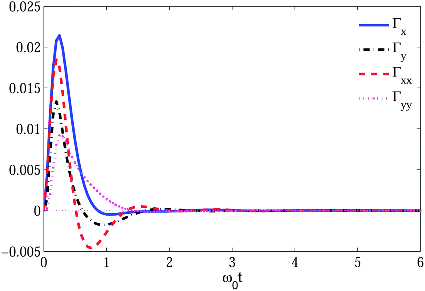


 numerical advantage.