
 Open Access Article
 This Open Access Article is licensed under a
 Creative Commons Attribution 3.0 Unported Licence
Plasmonic gold–poly(N-isopropylacrylamide) core–shell colloids with homogeneous density profiles: a small angle scattering study†
Martin
Dulle
a,
Sarah
Jaber
b,
Sabine
Rosenfeldt
a,
Aurel
Radulescu
c,
Stephan
Förster
a,
Paul
Mulvaney
b and
Matthias
Karg
*a
aPhysical Chemistry I, University of Bayreuth, Bayreuth, Germany. E-mail: matthias.karg@uni-bayreuth.de; Fax: +49 921 55 2780; Tel: +49 921 55 3920
bBio21 Institute & School of Chemistry, University of Melbourne, Melbourne, Australia
cJülich Centre for Neutron Science, Outstation at FRM II, Garching, Germany
First published on 19th November 2014
Abstract
Coating metal nanocrystals with responsive polymers provides a model case of smart, functional materials, where the optical properties can be modulated by external stimuli. However the optical response is highly sensitive to the polymer shell morphology, thickness and dielectric contrast. In this paper we study the nature of cross-linked, thermoresponsive polymer shells for the first time using four different scattering approaches to elucidate the density profile of the shells. Each scattering method provides unique information about the temperature-induced changes of shell thickness in terms of hydrodynamic radius and radius of gyration, the pair-distance distribution functions of the shells as well as the dynamic network fluctuations. Only a combination of these different scattering techniques allows to develop a morphological model of the core–shell particles. We further demonstrate control of the cross-linker distribution in core–shell synthesis by semi-batch precipitation copolymerization. Conducting the polymerization in three steps, we show for the first time that the polymer shell thickness can be successively increased without affecting the shell morphology and response behavior.
1 Introduction
Nanostructures which exhibit localized surface plasmon resonances (LSPR) have gained significant attention due to their unique optical properties which lend themselves to applications in sensing,1–6 plasmonic waveguiding7–9 and as light harvesting structures in photovoltaics.10–13 For these examples nanostructures with tailored optical properties are typically required, i.e. the LSPR must be tuned to a precise energy range. While this can be achieved by controlling the size, shape and composition of the objects, LSPR modes are also sensitive to the inter-particle separation3,14,15 and the refractive index of the surrounding environment.3,16–18 The inter-particle separation becomes important if optically functional materials shall be prepared via assembly of plasmonic nanoparticles since plasmon resonance coupling at low particle separations will strongly alter the absorption and scattering properties of the particle array. Shelling plasmonic nanoparticles with dielectric spacer materials has been shown to a powerful means for modulating the optical properties of particle assemblies by controlling the spatial separation between the nanoparticles. However, the encapsulation by a dielectric material will affect the LSPR due to the variation in the surrounding refractive index. This variation becomes particularly complex for polymer-coatings because their radial density profile is usually inhomogeneous. Thus the refractive index is not constant in such a shell which makes a prediction and theoretical description of the LSPR properties of the plasmonic core–shell particles difficult. Conversely polymer encapsulation is a frequently used strategy because it can be achieved rather easily via ligand exchange19–21 or polymerization in the presence of the plasmonic nanoparticles.22,23 Furthermore polymer encapsulation allows the realization of inter-particle separations from a few nm up to a few hundred of nm. A versatile coating material for plasmonic nanoparticles such as gold and silver is cross-linked, thermoresponsive poly-(N-isopropylacrylamide) (PNIPAM).24–26 The free-radical polymerization of the monomer NIPAM at temperatures above the lower critical solution temperature (LCST) of PNIPAM (32–33 °C) allows for nanoparticle encapsulation since the growing oligomer chains, at the early stages of the reaction, can precipitate onto the nanoparticle surface. It has been shown that such a PNIPAM shell represents a soft spacer which can be employed to control the inter-particle separation in particle monolayers27 and 3D nanocrystal superlattices.28 This separation depends directly on the thickness of the polymer shell. Karg et al. have shown that the monomer concentration in the polymerization step can be used to tune the PNIPAM shell thickness on gold nanoparticle cores.25 These authors have also shown that the optical properties of such inorganic–organic core–shell particles depend strongly on the shell thickness as well as the amount of the cross-linker N,N′-methylenebisacrylamide (BIS) used in the synthesis. However, a quantitative theoretical description of the optical properties is difficult because this requires knowledge of both the shell thickness and the shell morphology.While control of the shell thickness is possible, control over the internal structure remains challenging. Wu et al. studied the kinetics of the polymerization of NIPAM and BIS and found a quicker consumption of the BIS molecules as compared to NIPAM.29 Hence a rather inhomogeneous cross-linker distribution in these PNIPAM microgels is expected with higher cross-linked domains in the interior and a decreased degree of cross-linking towards the particle surface. Indeed such an inhomogeneous structure was revealed by small angle neutron scattering (SANS) of dilute microgel dispersions by Fernández-Barbero et al. pointing to a core–shell type structure with a dense core containing most of the cross-linker and a shell of lower density.30 This was corroborated by a detailed SANS investigation of the microgel form factor by Stieger et al.31 For measurements in the swollen state the authors identified a density profile with nearly constant density in the interior (box profile) and a rather large exterior volume with decaying density (error function). For a PNIPAM microgel prepared with 5.5 mol% BIS and relatively small dimensions (115 nm hydrodynamic radius, swollen) they found a radius of 38 nm for the inner, highly cross-linked part (box profile) and an exterior region with decaying density of 68 nm total thickness. In other words the inner volume with a rather homogeneous structure is significantly smaller than the outer inhomogeneous part. More recently Reufer et al. revealed the inhomogeneous network structure of PNIPAM microgels cross-linked with BIS by using dynamic light scattering (DLS) and static light scattering (SLS).32 Karg et al. used DLS and SANS to study PNIPAM microgels prepared with different contents of BIS.33 They found a rather strong dependence of the swelling behavior and the scaling behavior of the correlation length ξ on the cross-linking content. Their results indicated that the network homogeneity decreases with decreasing cross-linking. This was also shown by Varga et al. using SLS and DLS to investigate the structural inhomogeneities of PNIPAM microgels.34 These authors demonstrated that the particle structures for low cross-linking densities have a core–shell type morphology with a shell of lower density whereas a more homogeneous structure is found for higher cross-linking. However it remains a challenge to visualize the network morphology of microgels in real space. Gawlitza et al. have indirectly confirmed the presence of differently sized meshes in PNIPAM microgels of different cross-linking by loading experiments with gold nanoparticles.35 For weakly cross-linked microgels the gold nanoparticles of approximately 20 nm in diameter were distributed nearly homogeneously in the microgels upon incubation with the nanoparticles. However for microgels prepared with 5 and 10 mol% of cross-linker BIS, the gold particles were inhomogeneously distributed in the microgels, i.e. for the highest cross-linking studied the particles were distributed mainly in the outer microgel regions. This suggests the presence of meshes smaller than the gold particle diameter in the inner microgel region and an outer region with a larger mesh size where the gold particles are trapped. This example illustrates that understanding the network morphology is crucial if microgels are to be considered as carrier systems. To circumvent the presence of a strong cross-linking gradient semi-batch polymerizations were performed by different authors. Meyer and Richtering have shown that a semi-batch synthesis of PNIPAM microgels leads to microgels with a more homogeneous internal network morphology as compared to simple batch polymerizations.36 The difference in network structure was revealed by form factor analysis of SLS data. Later Acciaro et al. used a monomer feeding protocol to synthesize PNIPAM microgels with a homogeneously cross-linked network structure as analyzed by DLS and the optical appearance of microgel dispersions.37 To obtain micrometer sized microgels with homogeneous networks, Still et al. performed semi-batch polymerizations using a cationic comonomer that controls the charge concentration on the seeds during the polymerization.38 These authors used SLS to study the structure of their fairly large microgels. The SLS profile could be described by the core–shell model derived earlier by Stieger et al.31 and revealed an inner, homogeneous microgel section with a radius of 495 nm and a thickness of 324 nm for the outer layer with decaying density profile.
In this work we have used for the first time a semi-batch precipitation polymerization approach in the presence of gold nanoparticle seeds in order to control the characteristic polymer network length scales, i.e. the global size and the internal network structure, in structurally well-defined core–shell colloids. We applied three successive polymerization steps to obtain inorganic–organic hybrid particles with different overall dimensions determined by different polymer shell thicknesses in the sub-micrometer range. Scattering techniques employing light, X-rays and neutrons, covering in total a range of momentum transfer of almost three orders of magnitude, were performed to investigate the particles on the length scales of relevance.
2 Experimental section
2.1 Chemicals
N-Isopropylacrylamide (NIPAM; Aldrich, 97%), N,N′-methylenebisacrylamide (BIS; Fluka, ≥99.5%) and potassium peroxodisulfate (PPS; Fluka, ≥99.0%) were used without further purification.Gold(III) chloride trihydrate (Sigma-Aldrich, ≥99.9%), sodium citrate dihydrate (Aldrich, ≥99%), sodium dodecylsulfate (SDS; Ajax Laboratory Chemicals, Techn.) and butenylamine hydrochloride (BA; Aldrich, 97%) were used as received. Water was purified using a Milli-Q-system (Millipore). The final resistivity was 18 MΩ cm.
2.2 Synthesis
The prepared nanoparticles were then surface functionalized with butenylamine (BA). BA attaches to the gold nanoparticle surface through the amine, thus providing exposed free double bonds on the surface of the nanoparticles. Prior to the functionalization with BA, SDS was added to prevent aggregation induced by the increase in hydrophobicity caused by the BA coating. In addition we found that the SDS significantly helps to increase the colloidal stability upon concentration and purification by centrifugation. Without the addition of SDS, the gold nanoparticles are much more likely to aggregate during centrifugation. For a 200 mL amount of the previously prepared gold particle dispersion we added 1.2 mL of a 0.624 mM aqueous SDS solution dropwise under continuous stirring. After 20 min following the SDS addition, 0.392 mL of a 2.88 mM butenylamine hydrochloride solution in ethanol were added dropwise and stirring was continued for 20 min. The amount of BA corresponds to 3/4 of a monolayer assuming a surface coverage of 1 molecule per 0.4 nm2. Finally, the gold nanoparticles were concentrated by centrifugation, which was performed for 90 minutes at 3300 RCF. After centrifugation the supernatant was removed leaving only a few droplets of residue with highly concentrated gold nanoparticles. Since the supernatant still contained gold nanoparticles as evident from the red color, centrifugation was repeated with the supernatants. In total four centrifugation steps were performed this way in order to remove the majority of gold particles from solution. The residues were collected by adding only a few droplets of water for complete redispersion. The highly concentrated, nearly black particle stock solution was stored in the dark at room temperature.
The yields of the syntheses were determined gravimetrically after freeze-drying of the samples. A residual water content of 10% was assumed for all three samples. The yields in terms of total mass of the core–shell particles in relation to the total mass of the reactants are 27% after the first, 60% after the second, and 71% after the third polymerization step. It is worth noting that these yields cannot be directly related to the monomer conversion during the synthesis, which is expected to be much higher. The yields refer to the mass of particles obtained after purification from unreacted monomers and non-covalently bound oligomers.
2.3 Characterization
![[thin space (1/6-em)]](https://www.rsc.org/images/entities/char_2009.gif) :1:1 mixture of H2O:NH4Cl:H2O2 for 20 min at 70 °C. Monolayers of the samples were deposited by spin-coating of dilute, aqueous dispersions.
:1:1 mixture of H2O:NH4Cl:H2O2 for 20 min at 70 °C. Monolayers of the samples were deposited by spin-coating of dilute, aqueous dispersions.
![[capital Gamma, Greek, macron]](https://www.rsc.org/images/entities/i_char_e0ba.gif) . The polydispersity index was determined by cumulant analysis of autocorrelation functions measured at 60° scattering angle and sample temperatures of 6 and 58 °C. The samples were prepared by dissolving freeze-dried material and subsequent dilution to reach highly dilute conditions (ϕeff < 10−4). All samples were filtered using PTFE syringe filters with a pore size of 5 μm and filled into dust-free, cylindrical quartz cells.
. The polydispersity index was determined by cumulant analysis of autocorrelation functions measured at 60° scattering angle and sample temperatures of 6 and 58 °C. The samples were prepared by dissolving freeze-dried material and subsequent dilution to reach highly dilute conditions (ϕeff < 10−4). All samples were filtered using PTFE syringe filters with a pore size of 5 μm and filled into dust-free, cylindrical quartz cells.
In addition the scattering curves were fitted using the SASfit program by Kohlbrecher.42
3 Analysis of small angle scattering data
In a typical small angle scattering (SAS) experiment, the time-averaged scattering intensity is recorded as a function of scattering angle θ. The length scales which are resolved in the experiment depend on the range of values of the momentum transfer q. The de Broglie wavelength of the incoming beam (e.g. neutrons or X-rays) and θ define the magnitude of the momentum transfer q as follows: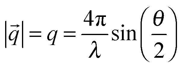 | (1) |
3.1 SANS profiles of cross-linked microgels
First of all we will describe the small angle scattering profiles of purely organic, cross-linked microgels and neglect the gold core present in our core–shell system. This assumption is actually reasonable for neutron scattering due to the low scattering contrast of gold in heavy water (Δη = 1.7 × 10⁻⁶ Å−2) and the very low volume fraction of the gold core with respect to the overall core–shell particle volume (below 1% for all samples).Scattering profiles for cross-linked polymer gels are typically determined by a static and a dynamic contribution:43
| I(q) = Istat(q) + Idyn(q) + Iinc | (2) |
I inc is the incoherent background, which was found to be nearly independent of q in the studied q-range and thus could be subtracted from the SANS profiles as a simple offset. Istat(q) is directly related to the presence of cross-linker points in the network. In contrast, the dynamic contribution Idyn(q) is caused by local concentration fluctuations44 (Ornstein–Zernicke contribution) due to the liquid-like nature of the gel. Since these fluctuations appear typically on a length scale of a few nm, the dynamic contribution to the scattered intensity is observed at relatively large q. These liquid-like contributions can be well-described by a Lorentzian function:45
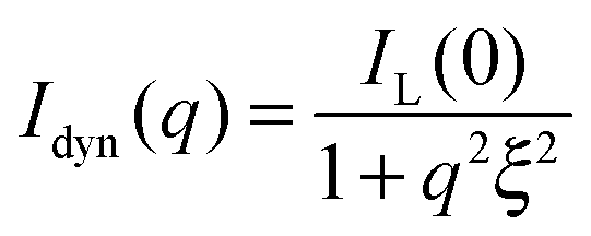 | (3) |
Here, IL(0) is the Lorentzian intensity and ξ the correlation length. For good solvent conditions ξ is often referred to as the blob size of a gel.30,45,46 It has been shown experimentally that ξ depends on the network connectivity at a given swelling state of the network.43 Furthermore ξ scales with the volume fraction of polymer, which has been experimentally revealed for cross-linked PNIPAM microgels by Stieger et al.47
For microgel particles with dimensions in the range of a few hundred nm the low q-part of the scattering profiles is dominated by the particle form factor P(q). For spherical, non-interacting particles with radius R under dilute conditions, P(q) is given by:
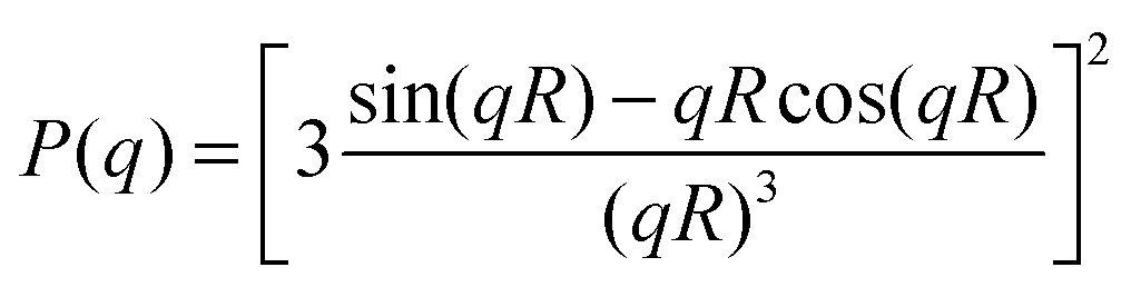 | (4) |
To account for polydispersity of the spherical particles this form factor is typically convoluted with a size distribution function (e.g. Gaussian size distribution). It has been shown in the literature that the form factor of polydisperse spheres is not sufficient to describe the low q-part of the scattering profiles of microgels.31,47 This is related to an inhomogeneous network structure where the density profile deviates from the simple box profile valid for hard spheres. In contrast to microgels from a simple batch polymerization which were found to have a rather pronounced gradient in cross-link density, the network morphology of microgels from a semi-batch approach is more homogeneous.36
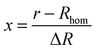
For our core–shell particles synthesized by a semi-batch process, we found that the density profile is rather homogeneous in the interior of the PNIPAM shell, but decreases in the outer region of the shell. To account for this density decrease we used a form factor model with an exponentially decaying scattering length profile ηexp(x) in the outer shell and a homogeneous scattering length profile in the homogeneous interior of the PNIPAM shell ηhom for the description of the experimental P(q).42 Depending on the sign of the exponent α, the exponentially decaying scattering length profile of the outer shell ηexp(x) is:
 | (5) |
In this equation x is the relative distance of a segment of the exponentially decaying density shell, with a thickness ΔR, to Rhom, the radius of the homogeneous shell section, according to:
 | (6) |
Furthermore, the scattering length density at Rhom is given by:
| ηin = ϕinηsolvent + (1 − ϕin)ηshell | (7) |
In the latter equation ηshell is the scattering length density of the pure shell material (cross-linked PNIPAM), ϕin the volume fraction of solvent with the scattering length density ηsolvent at r = Rhom and ϕout the volume fraction of solvent at r = Rhom + ΔR. The scattering length density at r = Rhom + ΔR is given by:
| ηout = ϕoutηsolvent + (1 − ϕout)ηshell | (8) |
Thus, the scattering length density profile with the homogeneous core and the decaying shell can be written as:
 | (9) |
The scattering intensity for such a radially symmetric scattering length profile is obtained by integration over r:
 | (10) |
The SANS profiles of our smallest particles, Au–PNIPAM-1, can then be fully described by the sum of eqn (3) and (10):
 | (11) |
For the larger particles Au–PNIPAM-2 and Au–PNIPAM-3, the form factor is not well resolved in the accessible low q part. The scattering intensity in the low q-part of the accessible q-range is then dominated by scattering from the particle/solvent interface. For a smooth interface Porod's law can be used to describe the profiles in this region:48,49
 | (12) |
Exponents for the q-dependence larger than the value of 4 in Porod's law indicate a rather rough interface.50
3.2 SAXS profiles of core–shell colloids
For our Au–PNIPAM core–shell samples, the contrast situation for scattering using X-rays is rather different compared to neutron scattering. The high electron density gold cores cannot be neglected here and apparently will dominate the high q scattering due to the relatively small size of the gold cores. In this q-range background corrected SAXS profiles can be described using a form factor for polydisperse spheres (e.g. using eqn (4) convoluted with a Gaussian size distribution). The scattering contrast of the gold cores in relation to the PNIPAM shell is so large that the liquid-like contributions to the scattering profile are not resolved. Only at the lowest q-values do the PNIPAM shells contribute to the SAXS curves. This can be sufficiently described by an additional polydisperse sphere form factor with the radius of the sphere accounting for the overall Au–PNIPAM particle radius. The polymer-free volume due to the presence of the gold core does not have to be accounted in this description due to the rather small volume of the cores compared to the PNIPAM volume. For core–shell particles with larger cores this situation will be different and a core–shell form factor needs to be used rather than the sum of two polydisperse sphere contributions.3.3 SLS profiles of core–shell colloids
A much lower q-range as compared to SAXS and SANS is available by light scattering due to the rather large wavelength of visible light. Hence, SLS can cover the low q part of the form factor. For all samples the Guinier region, providing the radius of gyration Rg, can be resolved: | (13) |
Here, I0 is the scattering intensity at q = 0 nm−1.
4 Results and discussion
Gold–PNIPAM core–shell particles were prepared by surfactant-free precipitation polymerizations of the monomer NIPAM and the cross-linker BIS in the presence of functionalized gold nanoparticles. The radical polymerizations were conducted above the LCST of PNIPAM. Under these conditions the monomers are still soluble in the reaction medium. Conversely short-chain oligomers will already phase separate and the gold nanoparticles will act as precipitation centers. Hence, the gold nanoparticles will be homogeneously encapsulated by cross-linked PNIPAM. In order to obtain polymer shells with a rather homogeneous network structure, i.e. with a homogeneous cross-linking in the interior of the shell, we performed the polymerizations in a semi-batch fashion with continuous feeding of monomer solutions. By dividing the feeding protocol into three steps we were able to prepare samples with three different shell thicknesses.4.1 Particle morphology
In order to study the successful encapsulation of the gold nanoparticles we investigated all samples by TEM. Fig. 1(A)–(C) shows TEM images of the three samples. Lower magnification images showing a larger number of particles can be found in the ESI† (Fig. S1). Due to the large difference in electron density (gold core vs. PNIPAM shell), the core–shell structure of the particles is clearly visible: the gold cores appear as dark circles homogeneously surrounded by a grey corona (polymer shell). The percentage of particles without a core is lower than 5%.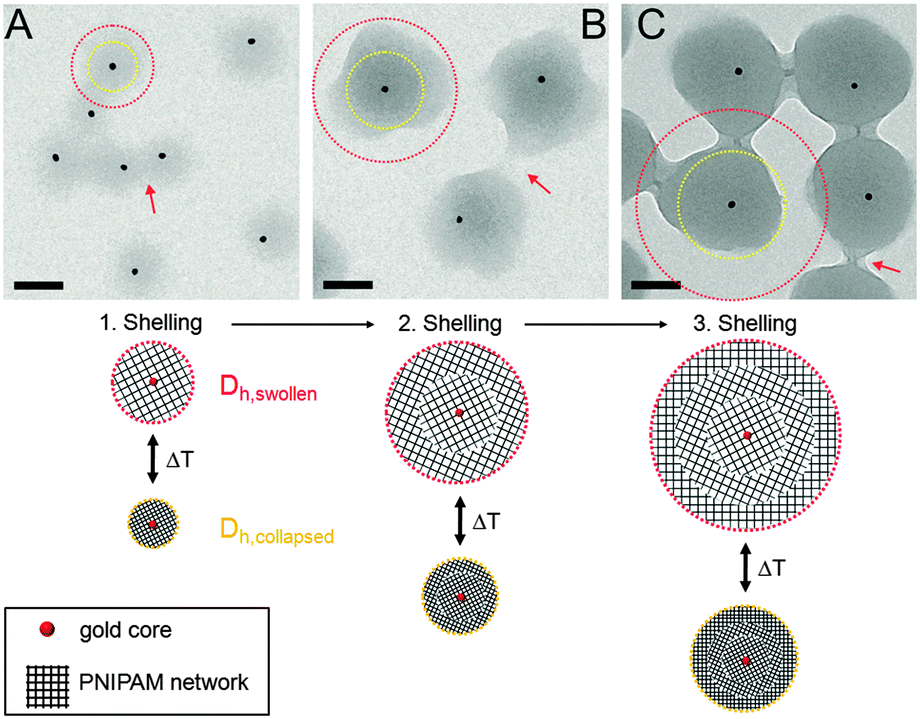 | ||
| Fig. 1 Top: TEM images of Au–PNIPAM-1 (A), Au–PNIPAM-2 (B) and Au–PNIPAM-3 (C). The red arrows indicate overlapping polymer segments of the fuzzy corona of particles in close vicinity. The scale bars correspond to 100 nm. Bottom: schematic depiction of the three different core–shell systems. The red dotted circles correspond to the hydrodynamic dimensions in the swollen state. The yellow dotted circles correspond to the hydrodynamic dimensions in the collapsed state. See Table 1 for values of the hydrodynamic radii. | ||
Furthermore the difference in shell thickness after each shelling step can be seen (increasing from A to C). In the following the three samples will be referred to Au–PNIPAM-1, Au–PNIPAM-2 and Au–PNIPAM-3 being the samples obtained after the first, the second and the third shelling, respectively. The red dotted circles in the TEM images highlight the overall particle dimensions in the swollen state determined by DLS from highly dilute (ϕeff < 10−4), aqueous dispersions, whereas the yellow dotted circles represent the dimensions in the fully collapsed state. The corresponding values for Rh are listed in Table 1. Details on the determination of Rh and the DLS analysis will be given in Section 4.3.
| Sample | R h (58 °C) [nm] | R h (6 °C) [nm] | M W (yield) [108 g mol−1] | M W (UV-vis) [108 g mol−1] |
|---|---|---|---|---|
| Au–PNIPAM-1 | 50 (51) | 83 (83) | 1.7 ± 0.2 | 1.5 ± 0.3 |
| Au–PNIPAM-2 | 78 (77) | 146 (149) | 9.1 ± 0.9 | 8.7 ± 1.4 |
| Au–PNIPAM-3 | 109 (111) | 194 (194) | 21.1 ± 2.0 | 20.1 ± 3.2 |
The dimensions of the particles imaged by TEM lie in between the hydrodynamic sizes in the swollen and collapsed state. This is due to the fact that the TEM images were recorded from particles adsorbed on a TEM grid under high vacuum conditions. The soft and fuzzy nature of the polymer shell is visible in areas where particles are in close vicinity and polymer chains seem to bridge the particles (highlighted by red arrows). These connections between neighboring particles are a result of the sample preparation. Under dilute dispersion conditions the particles are well separated and not agglomerated.
The schematic depictions in Fig. 1 illustrate the morphology of the three systems and are based on the experimentally determined particle size (according to DLS). After each shelling step an additional shell of cross-linked PNIPAM is added to the particles. This leads to a constant increase of the shell dimensions whereas the core–shell morphology remains unaffected. This can also be seen from AFM images shown in the ESI† (Fig. S2).
4.2 Optical properties
The optical properties of the core–shell particles were studied by UV-vis absorbance spectroscopy. Fig. 2 shows the spectra obtained from dilute, aqueous dispersions at 20 °C (swollen state) along with digital photographs of all three samples. The photographs show a red, almost clear particle dispersion for Au–PNIPAM-1. This red color arising from the LSPR of the gold nanoparticle cores (λmax = 518 nm prior to polymer encapsulation) is much less visible for Au–PNIPAM-2 and nearly invisible for Au–PNIPAM-3. At the same time Au–PNIPAM-2 and Au–PNIPAM-3 appear turbid. This tendency can also be observed from the spectra (solid lines). Au–PNIPAM-1 shows a well pronounced LSPR peak at around λmax = 523 nm. This value is redshifted by 5 nm compared to the gold nanoparticle cores before the polymer encapsulation. The redshift can be attributed to an increase in refractive index from water (n = 1.332) to water swollen PNIPAM (n > 1.332). Additionally the scattering contribution from the PNIPAM shell slightly affects the LSPR position since the scattering is wavelength dependent and will increase with decreasing wavelength causing the LSPR to appear slightly blue-shifted. The scattering from the polymer shell is visible in the spectrum of Au–PNIPAM-1 as an increase in absorbance towards wavelengths lower than the LSPR position. However, due to the relatively small dimensions of the Au–PNIPAM-1 particles the scattering from the PNIPAM shell is low. In contrast for Au–PNIPAM-2 the LSPR peak is much less intense and the rise in absorbance towards decreasing wavelength is much more pronounced. This means the scattering contribution for this sample is much stronger which is explained by the thicker PNIPAM shells and consequently larger overall particle dimensions. Due to the stronger scattering, the LSPR peak appears blueshifted (λmax = 521 nm) as compared to Au–PNIPAM-1. In case of Au–PNIPAM-3, which has the thickest PNIPAM shell, the LSPR is barely visible and its position cannot be easily determined. For this sample the scattering dominates the spectrum.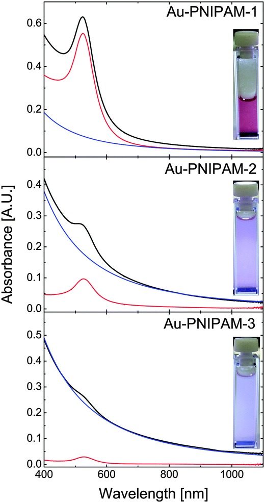 | ||
| Fig. 2 UV-vis absorbance spectra of the three core–shell systems. The black lines correspond to the core–shell spectra recorded at 20 °C. The blue lines are the modeled scattering contributions (RDG scattering) and the red lines are the modeled gold core absorbance spectra obtained by subtraction of the scattering contribution from the core–shell particle spectra. The insets show digital photographs of the samples in the quartz cells illuminated from the front. | ||
The scattering contribution of the PNIPAM shells was simulated by using simple power law fits according to Isc = Aλ−b, where Isc is the scattering intensity, A an amplitude factor and b the scattering exponent. This method has been used in a previous work already.25 The simulated scattering contributions are represented as the blue solid lines in Fig. 2. The values for A and b can be found in the ESI† (Table S1). Subtraction of the scattering contribution from the core–shell spectra allows us to determine the gold core spectra without the scattering contribution of the PNIPAM shells (red solid lines). The position of the LSPR should now be solely influenced by the refractive index environment. The positions are λmax = 524 nm for Au–PNIPAM-1, λmax = 526 nm for Au–PNIPAM-2 and λmax = 527 nm for Au–PNIPAM-3. More information on the analysis procedure can be found in the ESI† (Fig. S3).
The calculated spectra of the gold cores can now be used to determine the molar mass of the core–shell particles since we know the exact mass concentration of core–shell particles (freeze-dried, 10% residual water) in the UV-vis samples, the diameter of the gold cores from TEM and the extinction cross-section for Au0. This allows us to determine the number concentration of gold nanoparticles in the particle dispersions (in particles per L), and assuming 100% encapsulation of the gold cores by PNIPAM (no multiple cores, no empty microgels), the determination of the mass of the core–shell particles. The molar masses of the three samples calculated this way are listed in Table 1. The mass clearly increases with increasing shell thickness from sample Au–PNIPAM-1 to Au–PNIPAM-3. We also calculated the molar mass based on the yield of core–shell particles from the different reaction steps. For this calculation we again assumed 100% encapsulation of the gold cores. The values match very nicely to the values obtained from UV-vis analysis (see Table 1). This underlines the robustness of our approach, which is applicable to core–shell particles with fairly strong scattering contributions (Au–PNIPAM-3).
4.3 Hydrodynamic dimensions and swelling behavior
The overall dimensions of the core–shell colloids were investigated by dynamic light scattering (DLS). The detailed data analysis including angular dependent measurements can be found in the ESI† (Fig. S4–S6). All three core–shell systems show the typical VPT behavior of PNIPAM in water with transition temperatures around 33–35 °C. These values are slightly higher than for many reported PNIPAM microgels in water,33,49,51 which can be explained by the higher cross-linking content we employed. We have previously shown that the VPTT increases slightly with increasing BIS content.33 In addition the volume phase transitions of the samples are continuous with fairly broad transition ranges. This is also known for higher cross-linked microgels.33The hydrodynamic radii in the fully collapsed (58 °C) and the nearly fully swollen state (6 °C) obtained from CONTIN and cumulant analysis are listed in Table 1. As expected the hydrodynamic radii measured at 58 °C are significantly smaller than at 6 °C. In addition it is evident from Table 1 that the shell thickness increased after each polymerization step. Furthermore the second cumulant μ2 represents the variance of the relaxation rate distribution and can be used to determine the polydispersity  . The values for σ are <0.18 for all samples measured in the swollen and collapsed state.
To compare the VPT of each sample we calculated the deswelling ratio Vshell(T)/Vshell(swollen) for each sample and analyzed the temperature dependence. For this calculation only the volume of the PNIPAM shell was used Vshell(T) = Vcore–shell(T) − Vcore with Vcore calculated on the basis of the diameter from TEM analysis (13.2 nm). The hard gold core does not contribute to the swelling. The reference volume Vshell(swollen) was calculated using extrapolated values of Rh for T = 0 °C since not all samples reach a constant size in the low temperature range (6–20 °C) but rather swell slightly with decreasing temperature.
Fig. 3 shows the temperature evolution of the deswelling ratio. As can be seen the curves match very well for all samples except for some deviations of sample Au–PNIPAM-1 at temperatures above the VPTT. In this range the deswelling of Au–PNIPAM-1 is slightly less pronounced than for Au–PNIPAM-2 and Au–PNIPAM-3. This may be related to a slightly higher cross-linking efficiency for the sample after the first polymerization step. However the deviation is only small and an interpretation at this stage is difficult. For all samples the maximum degree of deswelling lies around 0.1–0.2, which means that the final hydrodynamic volume of the swellable PNIPAM shell has only 10–20% of its swollen volume.
 | ||
| Fig. 3 Results from CONTIN analysis of temperature dependent DLS measurements performed at a constant scattering angle of 60°. Relative change of the polymer shell volume Vshell with respect to the swollen state (reference state) as a function of temperature. | ||
The results from temperature dependent DLS measurements show a clear increase in particle size after each polymerization step with very similar deswelling behavior for all samples. This is a first indication of the similarity of the PNIPAM network morphology of each shell (see schematic depiction in Fig. 1 for a visualization of the shell morphology). However DLS only probes the translational diffusion of our core–shell particles which is related to the hydrodynamic volume. This method does not provide any information about the internal shell morphology. Therefore we performed SLS, SAXS and SANS measurements as well.
4.4 Radius of gyration, core radius and pair-distance distribution functions
Due to the relatively small overall diameter d of all three core–shell samples, SLS can be used to resolve the Guinier region for which the requirement qRg ≪ 1 typically needs to be fulfilled. Even for the largest sample, Au–PNIPAM-3, the Guinier region is resolved since the average refractive index of the water-penetrated PNIPAM shell is close to the refractive index of water. Hence the Rayleigh–Debye–Gans criterion is met although the particles do not fulfill the Rayleigh criterion for visible light (d < λ/20). Fig. 4(A) shows normalized SLS profiles for all samples measured at different temperatures. Sample Au–PNIPAM-1 only provided reasonable SLS profiles in the fully swollen state. This may be attributed to the small dimensions in the collapsed state and the low scattering intensity. SLS curves measured at higher temperatures were relatively noisy (even for very long acquisition times) and showed almost no angular dependence. Hence only results for 20 °C are shown for Au–PNIPAM-1.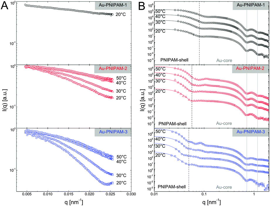 | ||
| Fig. 4 Results from temperature dependent SLS (A) and SAXS (B) experiments. Measurements were performed below (20 and 30 °C) and above the VPTT (40 and 50 °C). (A) SLS measurements normalized to I(q = 0 nm−1) = 1. (B) SAXS profiles and respective fits from IFT analysis (solid lines). The spectra were shifted horizontally by multiplication for the sake of clarity (×1, ×100, ×2000, and ×40000, from bottom to top). The solid, grey lines highlight the position of the form factor minima of the gold cores. The dashed, black lines highlight the position of the first form factor minima of the swollen core–shell particles (at 20 °C). | ||
All SLS profiles shown in Fig. 4(A) reveal angular dependence of the scattering intensity I(q). However the angular dependence of I(q) increases with increasing particle size from Au–PNIPAM-1 to Au–PNIPAM-3. The profile for Au–PNIPAM-1 at 20 °C shows only a slight but continuous decrease of I(q) with increasing q indicating that the low q-limit of the Guinier region is already probed. The form factor minimum of this fairly small sample is outside the accessible q-range and would appear at significantly larger q. In contrast to this, the first form factor minimum is already resolved by SLS for the largest sample, Au–PNIPAM-3, but only in the swollen state at 20 °C. With increasing temperature the sample Au–PNIPAM-3 shrinks and the form factor minimum shifts to larger q-values, which are again outside the accessible q-range. The particle shrinkage with increasing temperature leads to a decrease in the angular dependence of I(q). The same trend is observed for sample Au–PNIPAM-2. Since this sample is significantly smaller than Au–PNIPAM-3 the form factor minimum is not resolved even for the swollen state at 20 °C. Looking at sample Au–PNIPAM-2 and Au–PNIPAM-3 it appears that the SLS profiles measured at 40 and 50 °C do not significantly differ for each sample. This illustrates that the difference in size is almost negligible under these conditions. This is in agreement with the observation from DLS (see Fig. 3). From DLS the strongest change in particle size is observed comparing 30 and 40 °C. This effect is nicely reflected by the SLS profiles measured at these temperatures.
All SLS profiles shown in Fig. 4(A) were used to calculate the radius of gyration Rg from Guinier analysis according to eqn (13). The respective values for SLS experiments at 20 °C and the corresponding hydrodynamic radii Rh from DLS are listed in Table 2. We also calculated the ratio between both radii ρ = Rg/Rh. The values of ρ range from 0.70 to 0.73 and are close to the theoretically expected value of 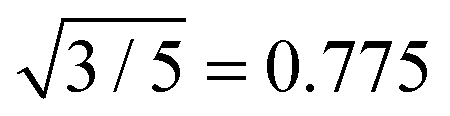 for hard spheres. We attribute the slightly smaller values to a low-density outer layer which may contain mainly linear chain segments. Such a layer will have an impact on the hydrodynamic radius probed in DLS but not significantly on Rg probed by SLS. This tendency has been also observed by Varga et al., who found values of ρ close to 0.6 for higher cross-linking contents (≈8 mol%).34 The cross-linking in this study is much higher and the values of ρ are significantly larger and closer to the hard sphere limit. We attribute this to a smaller exterior network domain with lower cross-linking.
| Sample | R h (20 °C) [nm] | R g (20 °C) [nm] | R g/Rh | R SAXS (20 °C) [nm] | R SANS (25 °C) [nm] |
|---|---|---|---|---|---|
| Au–PNIPAM-1 | 77 | 54 | 0.70 | 65 | 65 |
| Au–PNIPAM-2 | 135 | 98 | 0.73 | 100 | 100 |
| Au–PNIPAM-3 | 180 | 129 | 0.72 | 130 | 125 |
To study a broader q-range and to resolve the form factor of all samples, we performed SAXS experiments at comparable temperatures to the SLS experiments. The SAXS spectra are shown in Fig. 4(B). The solid lines in the spectra are fits from IFT analysis. The results from the IFT analysis will be discussed in Section 4.5. Looking at the high q-limit of the SAXS profiles at least two well-pronounced oscillations of I(q) are observed for all samples independent of the temperature. The two minima of I(q) which can be clearly identified (indicated by grey, vertical lines) are related to the form factor of the gold cores. The position of the first minimum is at qmin = 0.72 nm−1 which corresponds to a sphere radius of 6.2 nm. This value is in good agreement with the radius obtained by TEM (13.2 nm/2 = 6.6 nm). Due to the high electron density of the gold cores as compared to the PNIPAM shell, the SAXS profiles are dominated by scattering from the gold cores at q > 0.1 nm−1. It is worth noting that the measured samples were dilute (1 wt%) and the volume fraction of the gold cores is below 1% for all samples. Looking at the lower q-part of the profiles a sudden increase in I(q) with decreasing q is observed for all samples. This increase is related to scattering from the PNIPAM shell. The black dotted, vertical lines in the spectra highlight roughly the position of the first form factor minimum of the shell for each sample at 20 °C. The position of the minimum shifts to lower q for increasing particle size and hence the minimum has the lowest q value for Au–PNIPAM-3. For each sample the minimum shifts to larger values of q for increasing temperature. This effect is related to the temperature-induced shrinkage and hence a reduction in particle size of the core–shell colloids.
For the smallest sample Au–PNIPAM-1 the lowest accessible q values in the SAXS experiments are already sufficiently low to perform a Guinier analysis. Hence the radii of gyration which were not accessible by SLS for Au–PNIPAM-1 at 30, 40 and 50 °C can be determined. This allows us to analyze the dependence of Rg on the molar mass MW of the core–shell particles as determined by UV-vis analysis (see Table 1). In Fig. 5 the logarithm of Rg is plotted as a function of the logarithm of MW. A linear dependence is observed for all states of swelling. The slopes of the linear fits (solid black lines) provide the Flory exponent ν according to Rg ∝ (MW)ν. The values of the Flory exponent are ν = 0.34–0.39 for all temperatures. These values are very close to the theoretical value for hard spheres (ν = 1/3). This indicates a homogeneous network structure for all samples independent of the state of swelling.
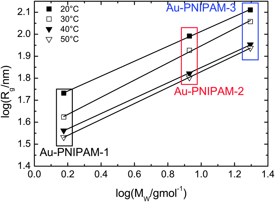 | ||
| Fig. 5 Analysis of the Flory exponent for different temperatures. Shown is the dependence of the radius of gyration (logarithmic) determined from SLS on the molar mass (logarithmic) as determined from UV-vis absorbance spectroscopy. The values of Rg for Au–PNIPAM-1 at temperatures higher than 20 °C were determined from Guinier analysis of SAXS profiles. | ||
4.5 Form factor analysis
Due to the high electron density of the gold cores in comparison to the PNIPAM shell, which only contains the light elements C, H, N and O, the scattering profiles from SAXS are dominated by scattering from the gold cores. However this contrast situation changes completely in the case of neutron scattering of the core–shell particles dispersed in heavy water. Fig. 6 compares results from SAXS and SANS experiments performed on dilute samples (1 wt%) dispersed in H2O and D2O, respectively. In Fig. 6(A) and (B) scattering profiles of all samples measured under good solvent conditions are shown (20 °C for SAXS and 25 °C for SANS). The solid lines in (A) and (B) are fits from IFT analysis. These fits describe the SAXS and SANS data of all samples very well. As discussed in the previous subsection the SAXS spectra of the core–shell samples are dominated by scattering from the gold cores although the volume fraction of the gold cores with respect to the overall particle volume is below 1% for all core–shell samples. For comparison a SAXS curve from the bare gold cores, prior to polymer encapsulation, is shown in (A) as well. Except for the low q regime, where scattering from the PNIPAM shell contributes, the gold cores show the same features as the profiles of the core–shell particles. The first two form factor minima are nearly at the same position as for the core–shell colloids. In contrast the scattering contribution of the cores is not visible in the SANS profiles shown in (B). The high q part is dominated by the dynamic fluctuations of the PNIPAM network (Ornstein–Zernicke contribution). At lower values of q two distinct form factor minima can be observed for Au–PNIPAM-1. For Au–PNIPAM-2 and Au–PNIPAM-3 the form factor minima are not well resolved. For these larger particles the minima are at the low q limit where the resolution in q is poor and the scattering features are smeared out due to the wavelength and geometrical instrument resolution. In Fig. 6(C) and (D) the normalized pair-distance distribution functions as obtained from IFT analysis of the SAXS profiles shown in (A) and SANS profiles in (B) are presented. These profiles were normalized to the maximum value of p(r) and to the maximum radius r for a direct comparison between the different core–shell samples. The values for the particle radii R corresponding to the values of rmax from this IFT analysis are listed in Table 2. Comparing the radii obtained by the different methods for the same sample a very good agreement is found. In addition, for Au–PNIPAM-2 and Au–PNIPAM-3 the radii from IFT analysis of the SAXS and SANS profiles are very close to the radii of gyration from SLS. For Au–PNIPAM-1 a deviation is observed with larger radii from IFT analysis as compared to the SLS analysis. For this sample the SLS characterization was difficult due to the rather small particle size and the weak scattering intensity leading to noisy SLS profiles with only small angular dependence indicating that SLS already probes the very low q-limit of the Guinier region for this sample. | ||
| Fig. 6 Results from small angle scattering performed at 20 °C. Left column: SAXS. Right column: SANS. (A) and (B) show scattering profiles with fits determined from IFT analysis (solid lines). (C) and (D) show normalized pair-distance distribution functions as a result of IFT analysis. (E) and (F) show small angle scattering profiles with fits obtained from form factor analysis using SASfit (solid lines). For the sake of clarity the SAXS profiles in (A) and (E) were shifted by multiplication (×1, ×100, ×2000, and ×40000, from bottom to top). The SANS profiles in (B) and (F) were also shifted by multiplication (×1, ×10 and ×100, from bottom to top). | ||
Comparing the pair-distance distribution functions of the different samples a very nice match of the profiles for SAXS as well as for SANS is found. This is an indication for very similar shell morphologies. All profiles are highly symmetric and their maxima are close to r/rmax = 0.5. Slight asymmetries for r/rmax between 0.75–1 may be explained by an outer region of lower cross-linking or even no cross-linking. The presence of such a layer was already estimated from results of Rg/Rh discussed previously in this subsection. The only noticeable difference comparing the pair-distance distribution functions from SAXS and SANS are the peaks at small relative radii in case of the SAXS profiles. These peaks are related to the gold cores. The intensity of the peak is decreasing with increasing PNIPAM shell size because the volume fraction of the core is decreasing. Pair-distance distribution functions obtained from SAXS without normalization to rmax can be found in the ESI† (Fig. S7). These profiles show that the peaks related to the gold core appear at very similar radii indicating that the core size is comparable between all samples. This highlights the robustness of the IFT analysis.
In addition to IFT analysis of the SAXS and SANS curves, we performed form factor fits using the software SASfit. In case of the SAXS profiles the form factor of simple spheres according to eqn (4) convoluted with a Gaussian size distribution could be used to sufficiently describe the large q-range of the core–shell profiles where the gold core scattering dominates. For the SAXS profile measured from the bare gold cores (black circles) this polydisperse sphere model describes the whole scattering profile very well (solid, grey line) providing a core radius Rcore = 6.5 nm with 8% polydispersity. This value is in very good agreement with the results from TEM analysis (Rcore = 6.6 nm, 8% polydispersity). The lower q-part of the profiles from the core–shell particles could be satisfyingly described by an additional polydisperse sphere form factor which accounts for scattering from the PNIPAM shell. These fits are shown as solid lines in Fig. 6(E) and provided core radii of Rcore = 6.3 nm for all core–shell samples. The overall radii from the form factor of the PNIPAM shell were 52, 78 and 96 nm for Au–PNIPAM-1, Au–PNIPAM-2 and Au–PNIPAM-3, respectively. The value for Au–PNIPAM-1 is in good agreement with the radius of gyration obtained from SLS and slightly smaller (≈20%) than the radius obtained from IFT analysis of the SAXS profile. For Au–PNIPAM-2 and Au–PNIPAM-3 the overall radii from SASfit analysis are significantly smaller than the radii obtained from SLS and IFT analysis of the SAXS profiles. This is related to the poor resolution of the form factor at low q for these relatively large particles.
The SANS data were analyzed using SASfit and different form factor models as well. In case of Au–PNIPAM-2 and Au–PNIPAM-3 the sum of a Lorentzian function (eqn (3)) accounting for liquid-like concentration fluctuations (Ornstein–Zernicke contribution) and a Porod part (eqn (12)) could be used to describe the scattering curves quite well. However, slight deviations from a value of 4 in the exponent were found in Porod's law (eqn (12)) indicating that the PNIPAM/solvent interface is not smooth.50 The exponents from the fits were 4.6 for both samples. Due to the very limited resolution of the form factor at small q for these rather large particles we did not analyze the data with a more complex model with more free fit parameters. Several authors have shown that the sum of eqn (3) and (12) can describe SANS profiles of cross-linked PNIPAM microgels.30,33,49,52
The form factor of Au–PNIPAM-1 is much better resolved at low q due to the much smaller dimensions of these particles. In a first attempt we fitted the SANS profile of this sample using a sum of a Lorentzian function (eqn (3)) and a form factor for spheres according to eqn (4) convoluted with Gaussian polydispersity. Whereas the Lorentzian function describes the high q-part of the profiles very well, the polydisperse sphere model could not describe the scattering functions sufficiently at low q. In contrast a form factor for spheres with an exponentially decaying profile in the exterior of the spheres according to eqn (10) could be used to describe the low q scattering. The full SANS profile of Au–PNIPAM-1 could thus be fitted by eqn (11) with Gaussian polydispersity used for Rhom. This fit provided Rhom = 28 nm, ΔR = 33 nm and α = −2.4. A value α = 0 would lead to a linear density decrease in the outer shell layer. Forcing α to 0 in the fitting process did not lead to a satisfying description of the scattering data. The volume fraction of solvent in the inner, homogeneous PNIPAM region is ϕin = 0.8. In other words the inner shell part is swollen by 80 vol% of solvent. This value is in very good agreement with the value of 82 vol% determined using the molar mass of Au–PNIPAM-1, the density of PNIPAM (ρ = 1.174 g cm−3, see e.g.ref. 53) and the particle radius based on SAXS and SANS (R = 65 nm). More details on the fit parameters and the different contributions of the form factor model to the scattering profiles can be found in the ESI† (Fig. S8 and Table S2).
4.6 Density profiles from SANS
The pair-distance distribution functions p(r) obtained from SANS measurements at 25 °C were convoluted into density profiles using the software DECON and a deconvolution procedure.54,55 A representative DECON fit can be found in the ESI† (Fig. S9). Fig. 7(A) shows the density profiles of the different core–shell particles. All profiles show a constant density at low radii, e.g. in the interior of the core–shell particles as typical for homogeneous spheres. In contrast at larger radii all profiles drop in an exponential fashion and the density decreases with increasing radius. This can be related to the lower cross-linked exterior of the core–shell particles. The presence of such a layer has already been experimentally observed for PNIPAM microgels prepared in classical batch syntheses.30,31,56 However, we would like to point out that the density profile of Au–PNIPAM-1 is already very similar to a box profile, i.e. these particles behave almost like hard spheres. The region where the density drops from 0.8 to 0 is only about 15 nm wide. Looking at Au–PNIPAM-2 and Au–PNIPAM-3 these regions are significantly larger (≈40 nm). This deviation may be due to the shelling procedure used for the particle syntheses but also due to the data analysis because of the poorly resolved form factors for these two, larger samples. Since the pair-distance distribution functions determined from SANS and SAXS analysis overlap very nicely for all three samples, we expect a rather similar shell morphology with lower cross-linked, outer regions of similar dimensions. | ||
| Fig. 7 Density profiles obtained from DECON analysis of SANS profiles (A) and from form factor analysis using SASfit (B). | ||
Fig. 7(B) shows the scattering length density profile relative to the solvent scattering length density (D2O) for sample Au–PNIPAM-1 as determined from SASfit analysis of the SANS profile using the form factor according to eqn (11). This profile matches very well with the profile obtained from DECON analysis. Again a constant density is found for the interior of the particles. At higher radii the density drops exponentially (α = −2.4) and reaches 0 at around 60 nm. The good agreement between the density profiles from DECON and form factor fitting demonstrates that the form factor model we have utilized in this study is well suited to describe the morphology of the core–shell particles. Due to the poor resolution of the rather large particles Au–PNIPAM-2 and Au–PNIPAM-3 and the limited accessible lower q values in the SANS experiment, scattering length density profiles for these two samples could not be generated. Only measurements on very low q instruments with a narrow wavelength distribution could provide the required scattering profiles for this analysis.
4.7 Internal network structure of the shells
Fernández-Barbero et al. have shown that the inhomogeneity of PNIPAM microgels can also be studied by analyzing SANS data in Ornstein–Zernicke representations.30 These authors determined three distinguishable regions in PNIPAM microgels from classical batch polymerization: a core region with a higher cross-linker density and smaller values of ξ, a shell region with lower cross-linking and larger values of ξ, and a surface region.Fig. 8 shows the Ornstein–Zernicke representations of the SANS profiles for all three core–shell microgels used in the present study.
 | ||
| Fig. 8 Ornstein–Zernicke representation of the SANS profiles measured at 25 °C in heavy water. The solid lines are linear fits. | ||
A single linear regime is found for all samples across a very wide range of momentum transfer values, q. Only at very low values of q is a deviation from linear behavior observed, which can be attributed to the form factor of the particles. Apart from this region the scattering profiles could be fitted linearly (solid lines) as shown in Fig. 8. The absence of other linear regions at lower q indicates that the majority of the PNIPAM shells are rather homogeneously cross-linked. The correlation lengths ξ determined from the intercepts and slopes of the linear fits are 1.5, 1.7 and 1.5 nm for Au–PNIPAM-1, Au–PNIPAM-2 and Au–PNIPAM-3, respectively. The effective volume fractions ϕeff of the core–shell particles in the samples examined by SANS can be calculated on the basis of the hydrodynamic radii at 25 °C and the molar masses of the colloids providing ϕeff = 0.06 for all samples. It is worth noting that the particles are highly swollen with solvent (D2O) under this condition and the actual polymer volume fraction will be in the order of 10 times smaller. Stieger et al. analyzed SANS profiles of PNIPAM microgels with 5.5 mol% of BIS at 25 °C and found a significantly larger value of ξ for comparable effective volume fractions. Our PNIPAM shells were prepared with a nearly 5 times higher content of BIS, which explains the lower values of ξ found for our systems. In a recent work we have shown that the correlation length of semi-dilute PNIPAM microgel systems decreases with increasing BIS content.33
4.8 Structural model for Au–PNIPAM core–shell particles
Applying DLS, SLS, SAXS and SANS to our Au–PNIPAM core–shell colloids provided information on different length scales, and with significantly different material contrasts. Fig. 9 shows a summarizing schematic depiction of the particle morphology as analyzed by the different scattering methods. The length scales in this example are drawn to scale for the Au–PNIPAM-1 sample, i.e. the core–shell dimensions are represented with the experimentally determined size ratios. | ||
| Fig. 9 Schematic depiction of the structure of the Au–PNIPAM core–shell particles with the gold core and PNIPAM shell dimensions drawn to scale with respect to sample Au–PNIPAM-1. The red circle in the center of the particle represents the gold core. The black, solid lines represent linear polymer chains and the cross-linker points are highlighted by grey circles. The experimentally determined radii from DLS (Rh), SLS (Rg), SAXS and SANS (RSAXS,SANS) and the core radius from SAXS and TEM (Rcore) are indicated. | ||
All core–shell particles studied in this work contain gold nanoparticle cores stemming from the same batch and hence with the same particle size and size distribution. The size of these cores was studied by TEM and SAXS prior to polymer encapsulation and by SAXS after the polymer encapsulation. The core radii and polydispersities determined before and after the shelling by polymer are in very good agreement.
The overall particle dimensions were studied by SAXS and SANS using IFT analysis as well as SLS using Guinier analysis. All radii were in good agreement for each sample except for the sample Au–PNIPAM-1. In the latter case the radii of gyration Rg from SLS were significantly smaller than the radii from IFT analysis of SAXS and SANS curves. This was attributed to uncertainities of the SLS profile and the respective Guinier fit obtained for this fairly small and weakly scattering sample. The hydrodynamic dimensions were studied by DLS providing values which have a smaller ratio in comparison to the radii of gyration as expected for simple hard spheres (Rg/Rh = 0.775). This was explained by the presence of a thin outer layer of low density, i.e. low or even no cross-linking, contributing to Rh but not significantly to Rg.
The internal structure of the polymer shell as depicted in the sketch shown in Fig. 9 was derived from DECON analysis of the pair-distance distribution functions obtained from IFT analysis of the SANS profiles. This approach revealed density profiles with constant densities in an inner shell region and an exponentially decaying density in the outer shell domains. This evolution of the density profiles was confirmed for Au–PNIPAM-1 by fitting the SANS profile with a corresponding form factor model.
Although the applied scattering techniques were not able to resolve the form factor of Au–PNIPAM-2 and Au–PNIPAM-3 with the same quality as for Au–PNIPAM-1, the results from all applied scattering methods suggest that the structure of the polymer shells of these samples is nearly identical to the Au–PNIPAM-1 sample.
The presence of a large inner shell volume with nearly homogeneous cross-linking was proved by Ornstein–Zernicke analysis of the SANS profiles for all samples. Hence the schematic structure shown in Fig. 9 can be derived for our core–shell particles prepared from semi-batch polymerization.
5 Conclusions
Network homogeneity in responsive, cross-linked polymer shells employed for encapsulation of plasmonic gold nanoparticles is accessible by sequential semi-batch polymerization. Gold nanoparticle seeds acting as precipitation centers during the free-radical precipitation copolymerization of N-isopropylacrylamide (NIPAM) and the cross-linker N,N′-methylenebisacrylamide (BIS) can be homogenously encapsulated by polymer where subsequent polymerization steps can be used to tailor the shell thickness without affecting its network architecture. We find that an outer shell region of lower crosslinking density cannot be avoided but a large inner volume of homogeneous density and hence homogeneous refractive index is achievable. A morphological model of these core–shell particles can only be derived using a combination of different scattering techniques. While the use of DLS is inevitable for following the swelling behavior based on the hydrodynamic particle dimensions, only a combination of SLS and SAXS provides the radii of gyration for the whole set of samples at different states of swelling. The form factor of the cores and the PNIPAM shells are accessible by SAXS at the same time, whereas only SANS resolves the dynamic fluctuations of the soft polymer shells.In a future study we will theoretically simulate the optical properties of these plasmonic core–shell particles using the density profiles derived in this work.
Although not in the focus of the present study, the gold cores present in our core–shell systems represent optically active centers allowing for spectroscopic detection and can also be used as a photothermally active source for microgel collapse.
Acknowledgements
PM thanks the ARC for support under Grant LF100100117. MK acknowledges financial support from the Fonds der Chemischen Industrie (FCI) via the Verband der Chemischen Industrie (VCI). MK and SF are grateful for financial support of the Deutsche Forschungsgemeinschaft through the SFB840.References
- Y. Kim, R. Johnson and J. Hupp, Nano Lett., 2001, 1, 165–167 CrossRef CAS.
- A. Haes and R. V. Duyne, J. Am. Chem. Soc., 2002, 124, 10596–10604 CrossRef CAS PubMed.
- C. Haynes, A. Haes, A. McFarland and R. van Dyne, Topics in Fluorescence Spectroscopy: Radiative Decay Engineering, Springer Science & Business Media, 2005, vol. 8, pp. 47–99 Search PubMed.
- R. A. Álvarez-Puebla, R. Contreras-Cáceres, I. Pastoriza-Santos, J. Pérez-Juste and L. M. Liz-Marzán, Angew. Chem., Int. Ed., 2008, 47, 1–7 CrossRef.
- E. D. Gaspera, M. Karg, J. Baldauf, J. Jasieniak, G. Maggioni and A. Martucci, Langmuir, 2011, 27, 13739–13747 CrossRef PubMed.
- M. Mueller, M. Tebbe, D. Andreeva, M. Karg, R. A. Puebla, N. P. Perez and A. Fery, Langmuir, 2012, 28, 9168–9173 CrossRef CAS PubMed.
- S. Maier, P. Kik, H. Atwater, S. Meltzer, E. Harel, B. Koel and A. Requicha, Nat. Mater., 2003, 2, 229–232 CrossRef CAS PubMed.
- W. Barnes, A. Dereux and T. Ebbeson, Nature, 2003, 424, 824–830 CrossRef CAS PubMed.
- R. Oulton, V. Sorger, D. Genov, D. Pile and X. Zhang, Nat. Photonics, 2008, 2, 496–500 CrossRef CAS.
- K. Catchpole and A. Polman, Opt. Express, 2008, 16, 21793–21800 CrossRef CAS PubMed.
- H. Atwater and A. Polman, Nat. Mater., 2010, 9, 205–213 CrossRef CAS PubMed.
- V. Ferry, J. Munday and H. Atwater, Adv. Mater., 2010, 22, 4794–4808 CrossRef CAS PubMed.
- Q. Gan, F. Bartoli and Z. Kafafi, Adv. Mater., 2013, 25, 2385–2396 CrossRef CAS PubMed.
- L. Liz-Márzan, Langmuir, 2006, 22, 32–41 CrossRef PubMed.
- A. Funston, D. Gómez, M. Karg, K. Vernon, T. Davis and P. Mulvaney, J. Phys. Chem. Lett., 2013, 4, 1994–2001 CrossRef CAS PubMed.
- P. Mulvaney, Langmuir, 1996, 12, 788–800 CrossRef CAS.
- L. Liz-Márzan, M. Giersig and P. Mulvaney, Langmuir, 1996, 12, 4329–4335 CrossRef.
- M. Müller, C. Kuttner, T. König, V. Tsukruk, S. Förster, M. Karg and A. Fery, ACS Nano, 2014, 8, 9410–9421 CrossRef PubMed.
- B. Ebeling and P. Vana, Macromolecules, 2013, 46, 4862–4871 CrossRef CAS.
- S. Ehlert, S. M. Taheri, D. Pirner, M. Drechsler, H.-W. Schmidt and S. Förster, ACS Nano, 2014, 8, 6114–6122 CrossRef CAS PubMed.
- M. Grzelczak, A. Sánchez-Iglesias and L. Liz-Márzan, CrystEngComm, 2014, 16, 9425–9429 RSC.
- D. J. Kim, S. M. Kang, B. Kong, W.-J. Kim, H.-J. Paik and I. Choi, Macromol. Chem. Phys., 2005, 206, 1941–1946 CrossRef CAS.
- C. Fernández-López, C. Pérez-Balado, J. Pérez-Juste, I. Pastoriza-Santos and L. Liz-Márzan, Soft Matter, 2012, 8, 4165–4170 RSC.
- R. Contreras-Cáceres, A. Sanchez-Iglesias, M. Karg, I. Pastoriza-Santos, J. Pérez-Juste, J. Pacifico, T. Hellweg, A. Fernández-Barbero and L. M. Liz-Marzán, Adv. Mater., 2008, 20, 1666–1670 CrossRef.
- M. Karg, S. Jaber, T. Hellweg and P. Mulvaney, Langmuir, 2011, 27, 820–827 CrossRef CAS PubMed.
- M. Müller, M. Karg, A. Fortini, T. Hellweg and A. Fery, Nanoscale, 2012, 4, 2491–2499 RSC.
- S. Jaber, M. Karg, A. Morfa and P. Mulvaney, Phys. Chem. Chem. Phys., 2011, 13, 5576–5578 RSC.
- M. Karg, T. Hellweg and P. Mulvaney, Adv. Funct. Mater., 2011, 21, 4668–4676 CrossRef CAS.
- X. Wu, R. Pelton, A. Hamielec, D. Woods and W. McPhee, Colloid Polym. Sci., 1994, 272, 467–477 CAS.
- A. Fernández-Barbero, A. Fernández-Nieves, I. Grillo and E. Lopéz-Cabarcos, Phys. Rev. E: Stat., Nonlinear, Soft Matter Phys., 2002, 66, 1–10 CrossRef.
- M. Stieger, W. Richtering, J. Pederson and P. Lindner, J. Chem. Phys., 2004, 120, 6197–6206 CrossRef CAS PubMed.
- M. Reufer, P. Díaz-Leyva, I. Lynch and F. Scheffold, Eur. Phys. J. E: Soft Matter Biol. Phys., 2009, 28, 165–171 CrossRef CAS PubMed.
- M. Karg, S. Prévost, A. Brandt, D. Wallacher, R. Klitzing and T. Hellweg, Prog. Colloid Polym. Sci., 2013, 140, 63–76 CAS.
- I. Varga, T. Gilányi, R. Mészáros, G. Filipcsei and M. Zrínyi, J. Phys. Chem. B, 2001, 105, 9071–9076 CrossRef CAS.
- K. Gawlitza, S. Turner, F. Polzer, S. Wellert, M. Karg, P. Mulvaney and R. Klitzing, Phys. Chem. Chem. Phys., 2013, 14, 15623–15631 RSC.
- S. Meyer and W. Richtering, Macromolecules, 2005, 38, 1517–1519 CrossRef CAS.
- R. Acciaro, T. Gilányi and I. Varga, Langmuir, 2011, 27, 7917–7925 CrossRef CAS PubMed.
- T. Still, K. Chen, A. Alsayed, K. Aptowicz and A. Yodth, J. Colloid Interface Sci., 2013, 405, 96–102 CrossRef CAS PubMed.
- J. Turkevich, P. Stevenson and J. Hillier, Discuss. Faraday Soc., 1951, 11, 55–75 RSC.
- I. Horcas, R. Fernández, J. M. Gómez-Rodríguez, J. Colchero, J. Gómez-Herrero and A. M. Baro, Rev. Sci. Instrum., 2007, 78, 013705 CrossRef CAS PubMed.
- G. Fritz, A. Bergmann and O. Glatter, J. Chem. Phys., 2000, 113, 9733–9740 CrossRef CAS.
- J. Kohlbrecher, SASfit: A program for fitting simple structural models to small angle scattering data, Paul Scherrer Institut, Laboratory for Neutron Scattering, CH-5232, Villigen, Switzerland, 2008 Search PubMed.
- A.-M. Hecht, R. Duplessix and E. Geissler, Macromolecules, 1985, 18, 2167–2173 CrossRef CAS.
- M. Daoud, J. P. Cotton, B. Farnoux, G. Jannink, G. Sarma, H. Benoit, C. Duplessix, C. Picot and P. G. de Gennes, Macromolecules, 1975, 8, 804–818 CrossRef CAS.
- M. Shibayama, T. Tanaka and C. C. Han, J. Chem. Phys., 1992, 97, 6829–6841 CrossRef CAS.
- M. Shibayama, T. Tanaka and C. C. Han, J. Chem. Phys., 1992, 97, 6842–6854 CrossRef CAS.
- M. Stieger, J. Pederson, P. Linder and W. Richtering, Langmuir, 2004, 20, 7283–7292 CrossRef CAS PubMed.
- H. Crowther, B. Saunders, S. Mears, T. Cosgrove, B. Vincent, S. King and G.-E. Yu, Colloids Surf., A, 1999, 152, 327–333 CrossRef CAS.
- K. Kratz, T. Hellweg and W. Eimer, Polymer, 2001, 42, 6531–6539 CrossRef.
- P. Wong, Phys. Rev. B: Condens. Matter Mater. Phys., 1985, 32, 7417–7424 CrossRef CAS.
- R. Pelton, Adv. Colloid Interface Sci., 2000, 85, 1–33 CrossRef CAS PubMed.
- S. J. Mears, Y. Deng, T. Cosgrove and R. Pelton, Langmuir, 1997, 13, 1901 CrossRef CAS.
- N. Dingenouts, S. Seelenmeyer, I. Deike, S. Rosenfeldt, M. Ballauff, P. Lindner and T. Narayanan, Phys. Chem. Chem. Phys., 2001, 3, 1169–1174 RSC.
- O. Glatter, J. Appl. Crystallogr., 1981, 14, 101–108 CrossRef.
- O. Glatter and B. Hainisch, J. Appl. Crystallogr., 1984, 17, 435–441 CrossRef CAS.
- B. Saunders, Langmuir, 2004, 20, 3925–3932 CrossRef CAS PubMed.
Footnote |
| † Electronic supplementary information (ESI) available: TEM bright-field images, AFM height profiles, analysis of the UV-vis absorbance spectra, intensity-time autocorrelation functions with cumulant fits, angular-dependent DLS results, hydrodynamic radii as a function of temperature, pair-distance distribution functions from SAXS, fit parameters from form factor analysis of SANS profiles, form factor contributions to the SANS profiles, and DECON fit of the pair-distance distribution function. See DOI: 10.1039/c4cp04816d |
| This journal is © the Owner Societies 2015 |