 Open Access Article
 This Open Access Article is licensed under a
 Creative Commons Attribution 3.0 Unported Licence
Electron transport in crystalline PCBM-like fullerene derivatives: a comparative computational study†
Julien
Idé‡
a,
Daniele
Fazzi
b,
Mosé
Casalegno
a,
Stefano Valdo
Meille
a and
Guido
Raos
*a
aDipartimento di Chimica, Materiali e Ingegneria Chimica “G. Natta”, Politecnico di Milano, via Mancinelli 7, IT-20131 Milano, Italy. E-mail: guido.raos@polimi.it; Fax: +39-02-23993180; Tel: +39-02-23993051
bMax-Planck-Institut für Kohlenforschung, Kaiser-Wilhelm-Platz 1, D-45470 Mülheim an der Ruhr, Germany
First published on 24th June 2014
Abstract
We present an extensive study of electron transport (ET) in several crystal forms of phenyl-C61-butyric acid methyl ester (PCBM) and 1-thienyl-C61-butyric acid methyl ester (ThCBM) fullerene derivatives. Our calculations are based on a localized representation of the electronic states. Orbital couplings, site energies and reorganization energies have been calculated using various density functional and semi-empirical techniques and used within the Landau–Zener, Marcus and Marcus–Levich–Jortner expressions to evaluate electron transfer rates. Electron mobilities have been then estimated by kinetic Monte Carlo (KMC) simulations. The adiabaticity of electron transfer directions within the different crystal structures has also been verified using the Landau–Zener expression. Finally, the role of low energy virtual orbitals of the fullerene molecules has been investigated using charge transport networks of increasing complexities. Our results show that these molecules may form one-, two- or three-dimensional percolation networks and that their higher energy orbitals often participate in ET. The highest mobility values were obtained for the crystal structure of ThCBM and are comparable to experimental values.
1 Introduction
The synthesis of [6,6]phenyl-C61-butyric acid methyl ester (PCBM) was first reported by Wudl and coworkers in 1995.1 Today, after almost two decades, PCBM is still the most popular n-type (i.e. electron transporting) material in organic electronics, often in combination with an electron donor polymer such as poly(3-hexylthiophene) (P3HT), as used inside the active layer of organic photovoltaic cells.2–5 It is likely that this enduring success would have surprised even PCBM's creators since, according to their original statements,1 at that time they were simply aiming at a soluble fullerene derivative which could be produced easily and cheaply, and be readily adapted for a variety of purposes through further functionalization reactions. Several attempts have been made to find good alternatives to PCBM,6–8 sometimes using relatively sophisticated “molecular design” approaches (including ab initio calculations, for example, to select candidates with suitable electron affinities), but none of them has really taken hold. As a result, it is still very pertinent to ask: what makes PCBM special? Liu and Troisi have recently come up with one possible answer to this question:9 unlike most other n-type materials, fullerene derivatives such as PCBM have anions with low lying excited states which may take part in charge separation at the interface with the donor polymer (exciton dissociation). This is interesting and useful, as it readily suggests a wide array of potential replacements for this material. On the other hand, this or any other design rule based on single-molecule properties cannot account for the full story, as they neglect all aspects related to molecular interactions and solid state organization, which are obviously crucial for properties such as processing and long-term stability, as well as charge and energy transport.10Several experimental studies have evidenced that the structural organization of PCBM in photoactive blends ranges from largely amorphous, to nanocrystalline, to highly crystalline structures,11–14 in which the solvent is thought to be absent.15 The relationship between the structural organization of PCBM molecules and their charge transport properties (electron mobilities, in this case) clearly represents a key issue. A typical approach would be to address it by computational methods, by first carrying out extensive molecular dynamics (MD) simulations, extracting atomistic models from them and finally computing these properties by simulating the drift-diffusion motion of the charge carriers.16–18 Indeed, in a previous study,19 we addressed the first part of this program by MD simulations of the structural organization of PCBM. Starting from the only two experimental crystal structures which were available at the time,20 respectively for a 1![[thin space (1/6-em)]](https://www.rsc.org/images/entities/char_2009.gif) :1 co-crystal with ortho-dichlorobenzene (DCB) and a 2:1 co-crystal with monochlorobenzene (MCB), we developed several models for amorphous, solvent-free PCBM by means of different combinations of solvent abstraction, heating and cooling. On the basis of these simulations, we concluded that a key property of PCBM is that, even in the amorphous state, it can form well-developed three-dimensional networks of electronically coupled fullerene molecules. Later on, Tummala et al.21 extended this study by carrying out further MD simulations and computing electron mobilities by kinetic Monte Carlo (KMC) simulations. More recently, other crystal structures have been added to the original pool, including the first solvent-free PCBM structure reported so far22,23 (these two papers discuss the same crystal structure, obtained respectively from powder and single-crystal X-ray diffraction) and that of the closely related ThCBM (1-thienyl-C61-butyric acid methyl ester),24 which is obtained from PCBM by replacing the phenyl with a thienyl group (see Fig. 1). Our group has identified also other PCBM polymorphs, including one containing dichloromethane (DCM).25 In parallel with these structural investigations, other authors have performed computational studies of the transport properties of fullerene-based materials. MacKenzie et al.26 combined MD and KMC simulations, demonstrating that longer side chains tend to interfere with electron transport. More recently, some authors have cast doubt on the applicability of the hopping models, arguing that the charge-localized picture which underlies this model is in fact inadequate for PCBM. Cheung and Troisi27 highlighted an unusual distribution of thermally accessible localized and delocalized states, which cannot be mapped onto standard models of transport in disordered media. Blumberger and coworkers28 computed electron transfer (ET) rates using a semi-classical rate expression including an adiabatic correction, and pointed out that the activation free energy for hopping can vanish for some strongly coupled fullerenes.
:1 co-crystal with ortho-dichlorobenzene (DCB) and a 2:1 co-crystal with monochlorobenzene (MCB), we developed several models for amorphous, solvent-free PCBM by means of different combinations of solvent abstraction, heating and cooling. On the basis of these simulations, we concluded that a key property of PCBM is that, even in the amorphous state, it can form well-developed three-dimensional networks of electronically coupled fullerene molecules. Later on, Tummala et al.21 extended this study by carrying out further MD simulations and computing electron mobilities by kinetic Monte Carlo (KMC) simulations. More recently, other crystal structures have been added to the original pool, including the first solvent-free PCBM structure reported so far22,23 (these two papers discuss the same crystal structure, obtained respectively from powder and single-crystal X-ray diffraction) and that of the closely related ThCBM (1-thienyl-C61-butyric acid methyl ester),24 which is obtained from PCBM by replacing the phenyl with a thienyl group (see Fig. 1). Our group has identified also other PCBM polymorphs, including one containing dichloromethane (DCM).25 In parallel with these structural investigations, other authors have performed computational studies of the transport properties of fullerene-based materials. MacKenzie et al.26 combined MD and KMC simulations, demonstrating that longer side chains tend to interfere with electron transport. More recently, some authors have cast doubt on the applicability of the hopping models, arguing that the charge-localized picture which underlies this model is in fact inadequate for PCBM. Cheung and Troisi27 highlighted an unusual distribution of thermally accessible localized and delocalized states, which cannot be mapped onto standard models of transport in disordered media. Blumberger and coworkers28 computed electron transfer (ET) rates using a semi-classical rate expression including an adiabatic correction, and pointed out that the activation free energy for hopping can vanish for some strongly coupled fullerenes.
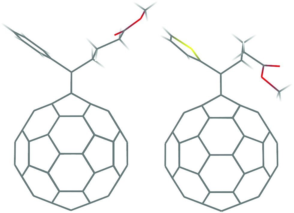 | ||
| Fig. 1 Molecular structures of PCBM (left) and ThCBM (right). | ||
The general aim of the present work is to contribute to the understanding of the relationship between the solid-state organization and the charge transport properties of fullerene derivatives. Are electron mobilities within these fullerene-based materials highly sensitive to the formation of a specific polymorph? Is charge transport more anisotropic in some forms than in others? Could this be hampered by the possible inclusion of solvent molecules? Do the low-lying virtual orbitals characterizing these materials play a role in charge transport? As our starting point, we have taken all the presently available experimental crystal structures of PCBM and ThCBM, which may or may not include solvent molecules. The latter is not as widely used as PCBM, but it is nonetheless very important from our point of view because of its high electron mobility (2 cm2 V−1 s−1 along one direction), as measured by time-resolved microwave conductivity on the same single crystals used for its structural determination.24 Electron mobilities have been evaluated using different versions of the hopping model for charge transport, despite its known limitations for fullerene-based materials.27,28 Compatible with these general aims and approach, we have tried to be as thorough as possible by checking the effect of different variables and computational assumptions. In particular, we have investigated: (1) the level of theory in the calculation of the electronic couplings (density functionals with different basis sets and semiempirical methods), (2) the intramolecular reorganization energies of different derivatives, (3) the effect of surrounding molecules on the site energies, (4) the adiabaticity of the electron hopping events, and (5) the complexity of the percolation network entering the KMC simulations, including the contribution of the fullerenes' low-lying virtual orbitals to ET.
2 Computational approach
We have adopted the approach reported in ref. 28 for the evaluation of the ET rates. On the basis of localized electronic states, we computed ET rates within different crystal structures using the same semi-classical rate expression and verified the non-adiabatic character of the different ET directions by calculating activation free energies. Note that the crystal structures were “frozen”, with all atoms at their experimental (average) positions. The inclusion of thermal fluctuation effects would have required extensive MD simulations of each crystal polymorph. The so-calculated ET rates were then used to perform KMC simulations to derive electron mobilities. For these simulations, percolation networks of various complexities were considered, including higher energy unoccupied orbitals on the fullerene derivatives.2.1 Electron transfer rates
The ET rates were calculated29 using the following semi-classical rate expression based on the Landau–Zener (LZ) treatment of non-adiabatic transitions28,30 (see the ESI† for a mathematical derivation):| kLZ = κelνeffexp(−β(ΔE‡na − Δ)) | (1) |
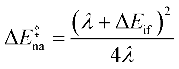 | (2) |
 | (3) |
In this expression, κel is the electronic transmission coefficient, νeff is the effective nuclear frequency, ΔE‡na is the non-adiabatic energy barrier and Δ is a correction factor relating ΔE‡na to the adiabatic energy barrier (ΔE‡ad = ΔE‡na − Δ). Hif and ΔEif = Ef − Ei are respectively the electronic coupling and site energy difference between the initial and final electronic states involved in the ET reaction, and λ is the total reorganization energy. β is 1/kBT, where kB is the Boltzmann constant and T is the absolute temperature.
We shall see that under specific conditions these equations predict negative adiabatic “barriers”. In such cases, we have still applied eqn (1) even though it can lead to ET which is faster than the vibrational time scale. This is an unphysical outcome of the localized hopping description, which however cannot be easily avoided at present.
The LZ approach was chosen to check the adiabaticity of ET directions, via the calculation of adiabatic barriers, consistently with other theoretical studies on PCBM.28 However, as many other workers in the field adopt the Marcus (non-adiabatic limit of the LZ expression) or the Marcus–Levich–Jortner (MLJ, quantum-mechanical treatment of non-adiabatic transfer reactions including tunneling effects) expressions, we also computed ET rates using them. In order to keep our discussion mainly focused on the comparison of the different crystal structures, the explicit expressions and the numerical results obtained with these rates are given in the ESI.† Overall, we can say that the electron mobilities deriving from the different expressions are comparable in magnitude and they tend to be in the order μMarcus < μLZ < μMLJ. The reasons for this are also discussed in the ESI.† Thus, even though it would be hard to say whether the LZ approach is really superior to the other two, it has at least the additional advantage of interpolating between them.
2.2 Electron transport simulations
KMC simulations were performed adopting the Bortz–Kalos–Lebowitz (BKL)31 algorithm to propagate a single charge carrier within the different crystal structures. For this purpose, we have developed an R-package32 for KMC simulations of charge transport, which has been released on “Comprehensive R Archive Network” (CRAN).29 The package also computes the necessary rate constant (LZ, Marcus or MLJ) from their basic quantum chemical ingredients. The mobility tensor![[small mu, Greek, macron]](https://www.rsc.org/images/entities/i_char_e0cd.gif) for each structure was calculated from the expression
for each structure was calculated from the expression ![[v with combining right harpoon above (vector)]](https://www.rsc.org/images/entities/i_char_0076_20d1.gif) = −
= −![[F with combining right harpoon above (vector)]](https://www.rsc.org/images/entities/i_char_0046_20d1.gif) , in which and are the applied electric field (|| = 106 V cm−1) and drift velocity vectors. The minus sign accounts for the fact that the charge carriers are negatively charged. Our choice for the electric field strength is discussed in the ESI,† which contains some numerical results for the field-dependence of the mobility in one of the crystal structures. Independent simulations with the electric field along the positive and negative x-, y- and z-directions were performed to build the mobility tensors. Each simulation lasted 107 hopping events and was repeated sixteen times with different random numbers (implying different initial positions of the charge). All our simulations were conducted by assuming that hopping events are restricted to neighbouring fullerene molecules, neglecting hopping to/from solvent molecules since these were found to display very high reorganization and site energies. Average hopping probabilities between each pair of molecules were extracted from these simulations and visualized.
, in which and are the applied electric field (|| = 106 V cm−1) and drift velocity vectors. The minus sign accounts for the fact that the charge carriers are negatively charged. Our choice for the electric field strength is discussed in the ESI,† which contains some numerical results for the field-dependence of the mobility in one of the crystal structures. Independent simulations with the electric field along the positive and negative x-, y- and z-directions were performed to build the mobility tensors. Each simulation lasted 107 hopping events and was repeated sixteen times with different random numbers (implying different initial positions of the charge). All our simulations were conducted by assuming that hopping events are restricted to neighbouring fullerene molecules, neglecting hopping to/from solvent molecules since these were found to display very high reorganization and site energies. Average hopping probabilities between each pair of molecules were extracted from these simulations and visualized.
The LUMO (L0), LUMO + 1 (L1) and LUMO + 2 (L2) orbitals are degenerate in C60 and they are relatively close in energy also in its derivatives PCBM and ThCBM. For both of them, ΔEL0L1 ≈ 0.06 eV and ΔEL1L2 ≈ 0.22 eV, while ΔEL2L3 ≈ 0.9 eV (B3LYP/6-31G* calculations). Since the thermal energy is kBT = 0.026 eV at room temperature, in principle they could also participate in the electron transport. Somewhat loosely, we may speak of “excited state conduction”, even though L1 and L2 are just one-electron functions which do not correspond to any true excitation of the molecules or their anions. In our view, their true role is to provide some additional flexibility in the description of the electrons' motion. We shall see that this partly compensates for the lack of thermal fluctuations in our structural models, by allowing some hopping events also among molecular pairs which would be forbidden on the basis of the L0 orbitals.
In our KMC simulations, for each neighbouring pair of molecules (defined on the basis of the coordination numbers reported in Table 1), an electron can be transferred along nine different pathways, related to the interaction between different orbitals centered on each fullerene (L0L0, L0L1, L0L2, L1L0, L1L1, L1L2, L2L0, L2L1 and L2L2). The results from this “F3-network” (where F indicates the full set of fullerenes, and 3 the number of orbitals per molecule) represent our standard for comparison with other, more approximate mobility simulations. First and foremost, they can be compared with more conventional KMC simulations based on a smaller network containing only the L0 orbitals of all molecules (“F1-network”). Within the lower-symmetry triclinic structures (see below), non-equivalent molecular sites can display significantly different L0, L1 and L2 energies. To determine to what extent the higher energy molecules contribute to ET, two further reduced percolation networks have been considered in the KMC simulations. The R3-network contains only the lower energy molecules, keeping all their three orbitals. The R1-network contains the same reduced set of molecules, keeping only their L0 orbital.
2.3 Electronic couplings and site energy differences
The electronic couplings and site energies were calculated by the fragment orbital approach described in ref. 33 and 34, using the ORCA35 and cclib36 packages. In this approach, for a single calculation the entire system is reduced to a dimer and the charge localization is mimicked by using the frontier orbitals of two isolated molecular fragments. In the case of an electron (hole) transfer, the Hamiltonian of the system is built in the basis of the LUMOs (HOMOs) of the monomers constituting the dimer. After re-orthogonalization,37 the site energies and transfer integral can be extracted respectively from the diagonal and off-diagonal terms of the transformed Hamiltonian. Thus, we extracted dimers for each ET direction within the different crystal structures and, using neutral state fragment-orbitals, electronic couplings and site energies were calculated at the DFT or semiempirical levels. We point out that, according to a recent paper with high-level hole transfer calculations on a series of small dimers,38 such fragment-based approaches can be expected to underestimate the electronic couplings by 20–30%.In the approach described above, site energies are calculated on molecular pairs and, since these depend on the dimer used for the calculation, they cannot be considered as true site properties. Furthermore, a calculation based only on dimers will tend to underestimate polarization effects.39 Another possible route may consist of using micro-electrostatic (ME) methods, as recently done to investigate energetics at the P3HT/PCBM interfaces40 and at the interface between donor–acceptor discotic liquid crystals.41 However, for the present work, ME methods cannot be used as site energies have to be computed for different virtual orbitals. Thus, to obtain better defined and more realistic values, we considered larger clusters centered on each site. To calculate the L0, L1 and L2 energies on a given molecule, we generalized the fragment orbital procedure by building a Hamiltonian for a cluster made up of that molecule with its L0, L1 and L2 orbitals, and its first coordination sphere with its L0 orbital. These site energies will be compared to those from pair calculations in the Results and discussion section.
2.4 Reorganization energies
The total reorganization energy involved in the electron transfer event investigated here is composed of an intra-molecular contribution λi and an outer sphere contribution λs arising from the change in the environment's polarizability and medium relaxation due to charge transfer:10| λ = λi + λs | (4) |
The intra-molecular contributions associated with the transfer of one electron were evaluated by using the adiabatic potential (AP) approach, which is also known as the “four point method”. The outer sphere contribution cannot be so easily estimated for charge transport processes in solid state media. In the past few years, some efforts have been made in this direction by the groups of Brédas,42 Troisi43 and Andrienko,44 who evaluated λs by hybrid QM/MM methods. However, only the class of acene compounds has been studied in depth. The use of continuum theory is another possible route, which has been followed by Gajdos et al.28 According to their evaluations, λs in PCBM crystals turns out to be in the range of 25–36 meV. In our study λs has been taken equal to 36 meV, the upper limit of this range, thus enhancing charge localization.
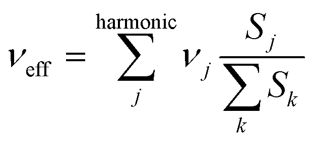
Another important parameter in eqn (1) is the effective nuclear frequency. To access this parameter, the Huang–Rhys (HR) factors Sj (electron–phonon coupling terms) have been computed from the displacement parameters (see the ESI†) as in ref. 45 and 46. Since low-frequency vibrations can be described to a good approximation in classical terms, and because of their possible anharmonicity47 (they are typically associated with large-amplitude librations around single bonds), the contributions for vibrational modes below 250 cm−1 were not included in the evaluation of the effective nuclear frequencies of PCBM and ThCBM. This cutoff falls below the lowest vibrational frequency of C60, so that all vibrations associated with the fullerene cage are treated quantum mechanically, and all the low-frequency “classical” vibrations are associated with the side groups. The effective nuclear frequency can then be written as:
 | (5) |
For the evaluation of λi and νeff, the hybrid B3LYP DFT functional and the double split 6-31G** basis set have been considered. The equilibrium geometries of the neutral and anionic states of the different species have been fully optimized, and the respective vibrational force fields have been evaluated to compute the HR factors. These calculations involved a standard, single-determinant representation of the electron density. In principle, a multi-configuration approach would have been more accurate (with an appropriate choice of the active space!) and consistent with our ET simulations including the low-lying L1 and L2 orbitals, but presently such calculations are still too demanding for molecules of this size. All these calculations have been carried out with the Gaussian09 program.48
3 Results and discussion
Overall, we have investigated six crystal structures. Four are PCBM co-crystals obtained by crystallization from dichloromethane (DCM),25 monochlorobenzene (MCB),20ortho-dichlorobenzene (DCB)20 and CS2,24 all of which contain guest solvent molecules. One is the solvent free structure (n-PCBM) recently described by our group22 (related to the one obtained from DCB) and the last one is a co-crystal of ThCBM, recently obtained from CS2 by Choi et al.24Table 1 summarizes the space group, the number of solvent molecule per unit cell as well as the PCBM (ThCBM) coordination numbers for each crystal structure (the latter can be defined as the number of fullerene molecules directly adjacent to a given one). Histograms (not shown) of the fullerene–fullerene distances were computed to determine a reliable cutoff (1.1 nm) for the definition of the first nearest-neighbours for each crystal structure. Four of the structures are monoclinic (P21/c or P21/n space groups). Their unit cells contain four PCBM molecules, all of which are related by symmetry. The two remaining structures are triclinic (P![[1 with combining macron]](https://www.rsc.org/images/entities/char_0031_0304.gif) space group) and they contain two non-equivalent pairs of symmetry-related fullerene molecules. In the triclinic structures we report two coordination numbers, respectively for the first and second sets of non-equivalent molecules, which in one case (ThCBM/CS2) are different from each other.
space group) and they contain two non-equivalent pairs of symmetry-related fullerene molecules. In the triclinic structures we report two coordination numbers, respectively for the first and second sets of non-equivalent molecules, which in one case (ThCBM/CS2) are different from each other.
In the following section we: (a) report the calculation of the reorganization energies and effective mode frequencies of PCBM and ThCBM and compare then with those of C60, (b) discuss the electronic couplings and site energies, including the effects of theory level and solvent molecules, and identify the conditions for the possible breakdown of the hopping model, (c) report and rationalize the mobility tensors corresponding to percolation networks of various complexities for each crystal structure.
3.1 Reorganization energies
The AP intra-molecular reorganization energy for C60 (used as a reference system for comparison), PCBM and ThCBM are reported in Table 2. Values for C60 and PCBM agree with literature data27,30,49 while for ThCBM this is, to the best of the authors' knowledge, the first evaluation of λi. C60 features the lowest reorganization energy among all the compounds, since the extra electron is fully delocalized over the π-electron carbon cage. PCBM and ThCBM show slightly higher reorganization energies (>0.015 eV) due to the phenyl and thienyl lateral groups which change locally the π-electronic structure of the fullerene and introduce extra vibrational modes in the charge relaxation process.| λ i/eV | hν eff/eV | ν eff/cm−1 | |
|---|---|---|---|
| C60 | 0.1356 | 0.1108 | 894 |
| PCBM | 0.1496 | 0.1612 | 1300 |
| ThCBM | 0.1510 | 0.1798 | 1450 |
To better understand the role of the local electron–phonon coupling parameters upon charge transfer, λi has been decomposed over all the vibrational normal modes of the neutral and charged species and both contributions (i.e. projection of the neutral geometry on the anion state and vice versa) are reported in Fig. 2 for each compound (numerical values are in the ESI†). We can observe that the introduction of the phenyl (PCBM) and thienyl (ThCBM) lateral group on the C60 carbon cage perturbs the local electron–phonon couplings changing those normal modes sensitive to the electron transfer process. Overall, the values of Sj terms are higher for PCBM or ThCBM with respect to the C60 case. PCBM and ThCBM present a few normal modes very sensitive (i.e. high reorganization) to the charge transfer process, showing HR factors of the order of 0.1. In particular, for PCBM we have the 903 cm−1 (S = 0.12), 1490 cm−1 (S = 0.09) and 1800 cm−1 (S = 0.06) active vibrations, while 902 cm−1 (S = 0.28), 1490 cm−1 (S = 0.095) and 1827 cm−1 (S = 0.16) for ThCBM. These vibrations represent C![[double bond, length as m-dash]](https://www.rsc.org/images/entities/char_e001.gif) C/C–C oscillations of the C60 cage and CO stretching of the carbonyl bond.
C/C–C oscillations of the C60 cage and CO stretching of the carbonyl bond.
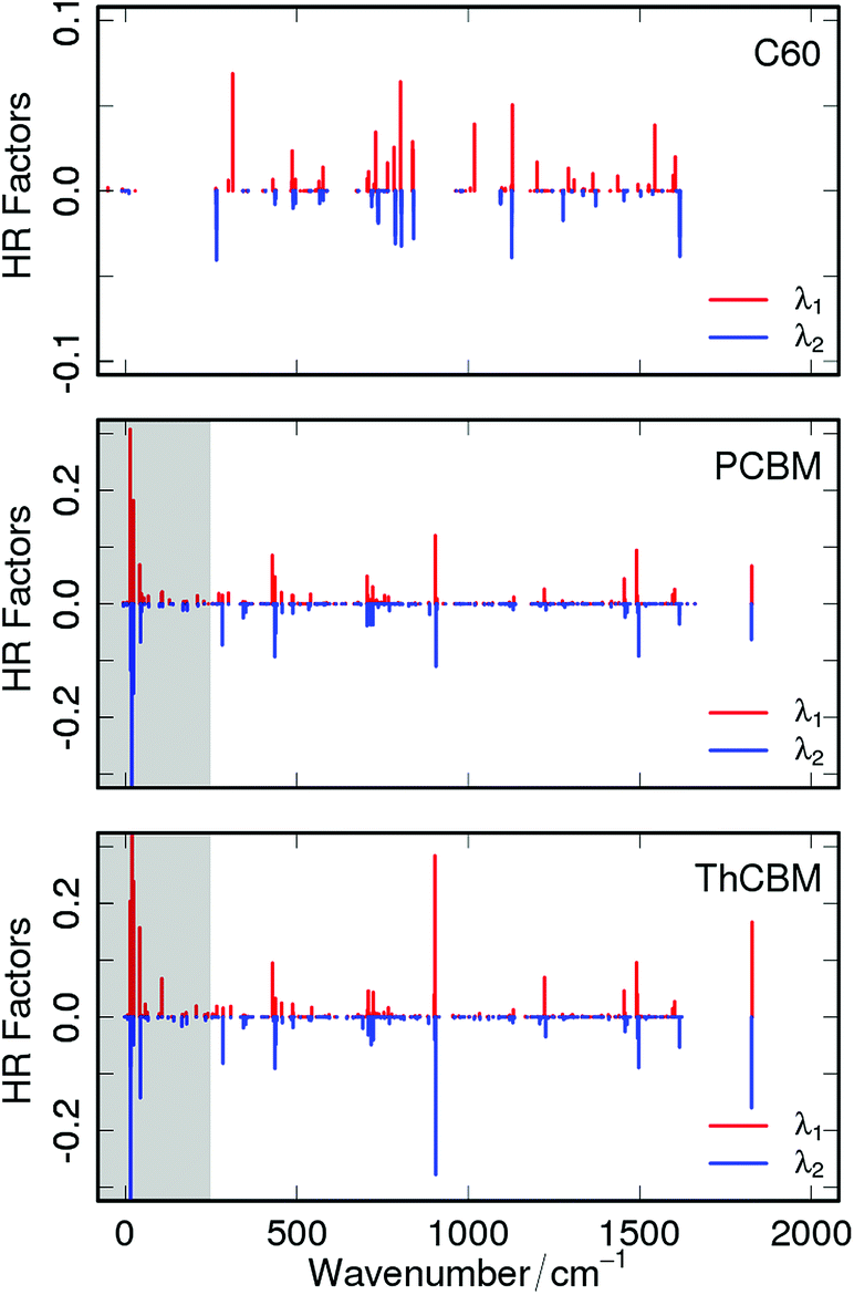 | ||
| Fig. 2 Computed B3LYP/6-31G** Huang–Rhys factors (|Sj|) for C60 (upper panel), PCBM (middle panel) and ThCBM (bottom panel). The grey area indicates the anharmonic region. Red and blue bins correspond respectively to the contributions of the neutral (λ1) and negatively charged (λ2) species. | ||
On the basis of these HR factors we computed the νeff values compiled in Table 2. The high effective frequencies obtained for PCBM and ThCBM reflect not only the higher reorganization energy with respect to C60 but also the high anharmonicity of low energy normal modes introduced by the side groups. The λi and νeff values reported in this section have been used in eqn (1), with the other ET parameters, for the evaluation of the rates.
3.2 Electronic properties and adiabaticity
Electronic couplings were calculated at the DFT level using the B3LYP functional and the 3-21G basis set. This choice was made on the basis of preliminary calculations on seven different PCBM dimers. The couplings between their L0, L1 and L2 orbitals were computed at the DFT level using the B3LYP and BLYP functionals and the 6-311G**, 6-31G*, 3-21G and STO-3G basis sets, and at the semi-empirical level using the ZINDO/S, AM1 and PM3 parameterizations.Fig. 3 shows a correlation diagram of these electronic couplings which demonstrates the substantial agreement among the DFT calculations, with the exception of those using a minimal basis set. The latter provide couplings which are intermediate between the non-minimal DFT and the rescaled AM1 or PM3 calculations (the correlations represented in Fig. 3 are independent of such scaling). It is also interesting to point out that, even if the ZINDO/S electronic couplings are comparable in magnitude to the DFT calculations (this is well known, and is one reason why they have been frequently used17,26,27), Fig. 3 indicates that ZINDO/S results do not correlate so well with DFT results. The scaling factor between the semi-empirical results and the DFT results obtained with the largest basis set (6-311G**) has been computed by linearly fitting the data obtained at each level of calculation plotted as a function of each other (not shown). The scaling factors (the slope of the linear fits) reported in Table 3 confirm that the ZINDO/S electronic couplings are closer to the DFT than AM1 or PM3.
 | ||
| Fig. 3 Correlation diagram (obtained with the “corrplot” library50 of the R project32) of the electronic couplings calculated between the L0, L1 and L2 orbitals of seven different PCBM dimers at different DFT and semi-empirical levels. | ||
| AM1 | PM3 | ZINDO/S | ||
|---|---|---|---|---|
| H ij | B3LYP/6-311G** | 4.37 | 6.63 | 2.43 |
| BLYP/6-311G** | 3.73 | 5.66 | 2.07 | |
| ΔEij | B3LYP/6-311G** | 1.12 | 0.97 | 1.19 |
| BLYP/6-311G** | 0.98 | 0.85 | 1.04 |
Site energies were estimated at the semiempirical level using the AM1 parameterization. This choice was dictated by the need to maintain reasonable computational times even for large clusters of fullerene and solvent molecules, which are responsible for sizeable polarization effects. A correlation diagram similar to Fig. 3 has been included in the ESI† (see Fig. S4) for the site energy differences. It demonstrates that, even though there are some differences among the computational levels, these are much more limited than for the couplings, since the correlation coefficients obtained from the dimer calculations are always comprised between 0.94 and 1. The scaling factors in Table 3 support our choice, as the AM1 parameterization is the one which provide the best fitting of the DFT results.
Fig. 4 collects the site energies for all crystal structures, in the cases with (a) isolated fullerene molecules, (b) fullerenes surrounded by their nearest neighbors, excluding the solvent molecules and (c) fullerenes with their nearest neighbors, including the solvent. In the latter case, when the solvent molecules have some positional/orientational disorder (PCBM/DCM and PCBM/MCB), site energies were calculated for all possible configurations. Finally, for the sake of comparison, we also give (d) the site energies extracted from the dimer calculations (i.e., those used for the evaluation of the electronic couplings).
 | ||
| Fig. 4 Site energies (L0 in red, L1 in green and L2 in blue) within the different crystal structures as calculated on (a) isolated fullerenes, (b) fullerenes surrounded by their first coordination spheres, removing solvent molecules, (c) fullerenes surrounded by their first coordination sphere, including solvent molecules and (d) fullerene dimers. | ||
The position of the L0, L1 and L2 levels calculated on isolated molecules depends on the crystal structure because of subtle differences in the PCBM (ThCBM) molecular geometries. In particular, the conformation of the PCBM and ThCBM side chains can lead to specific intra-molecular interactions which shift these levels. For the same reason, non-equivalent molecules in triclinic structures also present slightly different L0, L1 and L2 energies. The L0L0, L1L1 and L2L2 site energy differences between non-equivalent sites may be neglected when considering isolated molecules, but they become much larger when including polarization effects from neighbouring fullerene derivatives (b). Thus, the L0 and L1 as well as the L1 and L2 levels of non-equivalent sites may become very close in energy and they actually cross each other in the case of the ThCBM/CS2 structure (i.e., the L1 level of one molecule is lower than the L0 level of another, and similarly for the L2/L1 levels). The smallness of L0L1 and L1L2 site energy differences points to the possible contribution of the higher energy virtual orbitals to ET in the triclinic structures. At the same time, the site energies for the monoclinic structures suggest that only L0 contributes to ET. These indications have been checked by explicit KMC simulations, to be discussed below.
The inclusion of the solvent molecules in the coordination spheres (c) produces an additional shift of the fullerene levels. This shift appears to be more pronounced for the polar solvents. Indeed, when comparing the PCBM/DCM and PCBM/CS2 structures, which belong to the same space group and have very similar lattice parameters, we find that the levels of the PCBM/CS2 structure are almost unchanged while those of the PCBM/DCM structure are slightly shifted toward higher or lower energy, depending on the positions/orientations of the solvent molecules. This effect is even more pronounced for the PCBM/MCB structure, as the levels obtained for the different positions/orientations of the solvent molecules are spread to the point that they form a near-continuum structure. This is due partly to the polarity of MCB, partly to the fact that there are three solvent molecules surrounding each PCBM in this structure (DCM is also polar, but there are only two solvent molecules adjacent to the PCBM in the PCBM/DCM structure).
The calculations in case (c) show that, even though solvent molecules do not directly participate in charge transport (they have high energy orbitals and large reorganization energies), they might have an indirect effect by producing a spread in the fullerene orbital energies. However, the importance of this energy spread depends also on the solvent dynamics. For slow solvent reorientational motions, the electron would “see” a static distribution of energy levels whereas for fast solvent motions, it would feel an effective, narrower distribution centered about the average value. It turns out that the structure with the wider distribution (PCBM/MCB) is also the structure which, according to our previous MD simulations,19 has the fastest solvent rotations. For this reason, and for the sake of simplicity, we have neglected the solvent contribution to the site energies and used those from the (b) case in our KMC simulations.
The results of (d) case calculations on the fullerene dimers are rather far both from the isolated molecules and from the molecules within a large cluster. This confirms that the site energies from the dimer calculations are ill-defined and they cannot be used reliably in a KMC simulation.
Fig. 5 contains level plots of ΔE‡ad as a function of the orbital couplings and energy differences, for each crystal structure (in principle, the barrier depends also on the reorganization energies, but these are fixed parameters here). For some specific transport directions, we obtain negative adiabatic barriers for ET (points within the grey regions in the figure). This was observed also by Blumberger et al.,28 who justified this result on the basis of the inter-orbital couplings (for large couplings, an electron cannot be considered localized, as it spreads over strongly coupled molecules). However, these authors restricted their analysis to the L0L0 transfers and neglected the effect of site energy differences, even for the triclinic crystal structures with non-equivalent fullerene molecules. Our results for the sign of ΔE‡ad are somehow different from theirs, due to smaller electronic couplings and to the fact that our calculations include the effect of site energy differences. These cannot be neglected, both because we consider three orbitals instead of one and because some of our crystal structures (the triclinic ones) include PCBM or ThCBM molecules which are unrelated by symmetry.
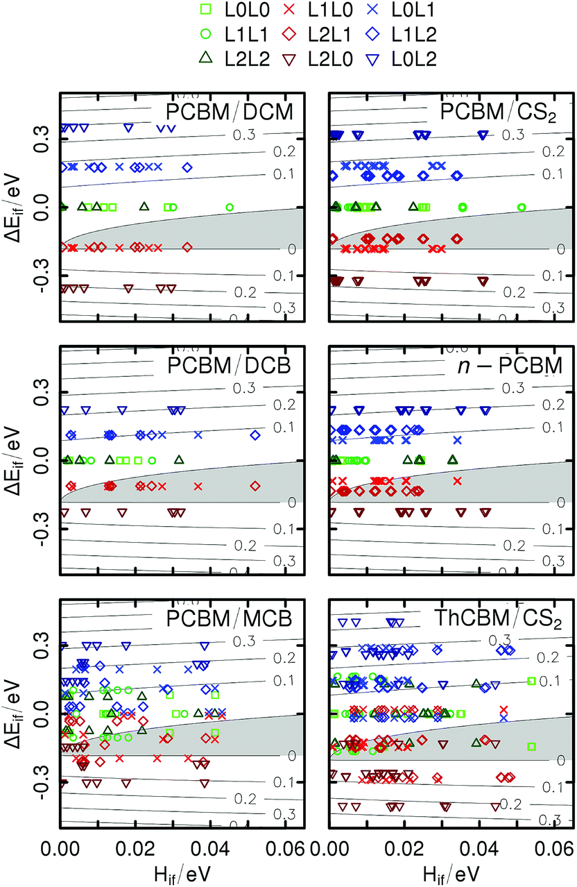 | ||
| Fig. 5 Level plot (in the [Hif, ΔEif] plane) of the adiabatic free energy barriers (in eV) for the different crystal structures. The grey area indicates the negative region of the plot. The green, red and blue symbols indicate respectively the flat, downward and upward ET directions. | ||
Three different types of ET can be distinguished in Fig. 5: “flat” (L0L0, L1L1, L2L2; green symbols), “upward” (L0L1, L1L2, L0L2; blue symbols) and “downward” (L1L0, L2L1, L2L0; red symbols). For the monoclinic structures, as no positional disorder has been introduced in our model, the flat, upward and downward ETs are respective athermal (ΔEif = 0), endothermal (ΔEif > 0) and exothermal (ΔEif < 0). For the triclinic structures, for which the L0, L1 and L2 levels of non-equivalent sites can cross each other, the sign of the site energy difference cannot be related any more to the type of ET (for example, there can be upward but exothermal L0L1 electron transfers).
It appears that for the monoclinic structures the ET pathways within the F1-networks defined in Section 2.2 (light green squares in the first four panels) never reach the negative region of the maps. This suggests that the hopping model is acceptable for these percolation networks including only LUMO–LUMO transitions. However, looking at the F3-networks (all red, green and blue points), a major part of the exothermal pathways (red points) display negative ΔE‡ad. For the triclinic structures, even the F1-networks display some negative barriers (light green squares in the last two panels), corresponding to ET between non-equivalent sites with different LUMO energies.
To summarize, in our model ΔE‡ad can be negative for two distinct reasons: (i) large electronic couplings, leading to charge delocalization as proposed by Blumberger and coworkers,28 but also (ii) large site energy differences, preventing charge localization on high energy sites even for fairly small electronic couplings. In principle, low energy fullerene sites may act as shallow traps driving ET. The KMC simulations will allow us to check this hypothesis.
3.3 Percolation networks
Using the electronic couplings, site energies and reorganization energies described in the previews sections, ET rates have been evaluated for each crystal structure according to the LZ expression (see the ESI† for the Marcus and MLJ rates). Rather than presenting large tables of numbers, which would be of limited interest due to the approximations in our calculations, we will resort to graphical representations produced with the “Rpdb”51 and “rgl”52 packages. These serve better our main purpose, that is, to get a feeling for the consequences of molecular packing on the ET properties of these fullerene derivatives.Fig. 6 presents the ET rates which define the F1-network for each crystal structure. The rates are represented by orange cones, whose tips point towards one molecule and whose bases are proportional to the rate to that molecule (i.e., the radius is proportional to the square root of the rate). The reader may think of them as funnels, channeling electrons towards their destination site. Note that the scaling factor connecting the size of the cones to the ET rates is the same of all crystal structures. Therefore, they provide a clear representation of the dimensionality of the percolation networks (one-, two- or three-dimensional transport), of the main electron transport directions, and of the relative ET rates within different crystal structures.
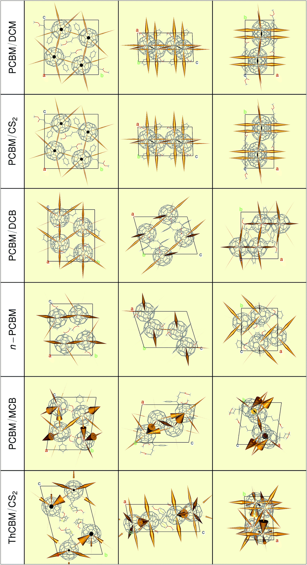 | ||
| Fig. 6 Representation of the Landau–Zener ET rates for the L0L0 transitions (cones with bases proportional to the rates, pointing towards the destination fullerene), forming the F1-networks. | ||
The cones in Fig. 6 show that the ET pathways within PCBM/DCM and PCBM/CS2 form a well-developed three-dimensional network, with a certain preference for the a-axis. Note the strong similarity between transfer networks in these two crystals, which reflects the analogy in their fullerene packings. Upon closer scrutiny, it turns out that the ET rates along a are actually 1.3 times larger in PCBM/DCM, in agreement with the slightly lower value of this lattice parameter. The two other monoclinic structures have lower dimensionality percolation networks. PCBM/DCB is essentially two-dimensional, in agreement with the alternation of PCBM and solvent layers along the (1 0 ) direction. Surprisingly, the n-PCBM network is the one with the lowest connectivity. The graphical representation of the rates indicates that the electrons may zig-zag comfortably only along the b-axis. A very short contact distance (2.9 Å) between PCBM molecules along that direction is at the origin of these zig-zags. Finally, the ET networks of the triclinic structures are more complex due to the presence of two distinct sets of non-equivalent fullerenes. The hopping rate from one to the other set can be one order of magnitude (or more) larger than the opposite one, and this is borne out by the very asymmetric double cones connecting them. It is difficult to decide on the dimensionality of their percolation networks by looking at these figures. In principle, the fullerenes at the end of the thickest cones might dominate charge transport.
The ET rates represented in Fig. 6 correspond to the L0L0 transitions forming the F1-networks. It is extremely difficult to obtain and interpret a similar representation of the F3-networks, which include transitions to/from the L1 and L2 orbitals (there are actually 18 such transitions between any pair of neighbouring fullerenes!). To understand the role of the higher energy orbitals and to answer some of the questions raised above, we carried out the KMC simulations described in the following section.
3.4 Electron transport simulations
To confirm and extend our previous conclusions on the charge transport properties of the crystals, which were based on the rates for the L0L0 transfers, we carried out KMC simulations on the F1- and F3-networks. For the triclinic structures, the role of high energy molecules was also investigated by constrained KMC simulations on the R1- and R3-networks. The numerical results for the electron mobilities are collected in Table 4 and, for the F1- and F3-networks, they are also represented graphically in Fig. 7.| Eigenvalues | Eigenvectors | Eigenvalues | Eigenvectors | ||||||
|---|---|---|---|---|---|---|---|---|---|
| x | y | z | x | y | z | ||||
| PCBM/DCM | PCBM/CS 2 | ||||||||
| F1 | 1.03 | −1.00 | 0.00 | 0.01 | F1 | 0.80 | 1.00 | 0.00 | −0.01 |
| 0.24 | 0.01 | 0.00 | 1.00 | 0.12 | 0.00 | 0.02 | 1.00 | ||
| 0.10 | 0.00 | −1.00 | 0.00 | 0.09 | 0.00 | 1.00 | −0.02 | ||
| F3 | 1.02 | −1.00 | 0.00 | 0.01 | F3 | 0.80 | 1.00 | 0.00 | 0.00 |
| 0.24 | 0.01 | 0.00 | 1.00 | 0.16 | 0.00 | 0.99 | 0.17 | ||
| 0.11 | 0.00 | −1.00 | 0.00 | 0.06 | 0.00 | −0.15 | 0.99 | ||
| PCBM/DCB | n-PCBM | ||||||||
| F1 | 0.37 | −0.43 | 0.00 | −0.90 | F1 | 0.45 | 0.00 | 1.00 | 0.00 |
| 0.27 | 0.00 | −1.00 | 0.00 | 0.02 | −0.59 | 0.00 | −0.81 | ||
| 0.00 | 0.90 | 0.00 | −0.43 | 0.01 | −0.80 | 0.00 | 0.60 | ||
| F3 | 0.44 | −0.43 | 0.00 | −0.90 | F3 | 0.54 | 0.00 | −1.00 | 0.00 |
| 0.38 | 0.00 | 1.00 | 0.00 | 0.11 | 0.81 | 0.00 | −0.58 | ||
| 0.00 | −0.90 | 0.00 | 0.43 | 0.08 | −0.61 | 0.00 | −0.79 | ||
| PCBM/MCB | ThCBM/CS 2 | ||||||||
| F1 | 0.30 | −0.62 | −0.19 | −0.76 | F1 | 1.49 | 1.00 | 0.00 | 0.00 |
| 0.05 | −0.74 | 0.50 | 0.46 | 0.02 | 0.00 | −1.00 | −0.08 | ||
| 0.05 | 0.53 | −0.81 | −0.24 | 0.00 | 0.00 | 0.00 | 1.00 | ||
| F3 | 0.36 | 0.59 | 0.10 | 0.80 | F3 | 1.48 | 1.00 | 0.00 | −0.01 |
| 0.15 | −0.11 | −0.98 | 0.15 | 0.07 | 0.00 | 0.50 | 0.87 | ||
| 0.08 | 0.82 | −0.15 | −0.55 | 0.03 | 0.00 | 0.92 | −0.40 | ||
| R1 | 0.07 | 1.00 | 0.00 | 0.00 | R1 | 1.45 | 1.00 | 0.00 | 0.00 |
| 0.00 | 0.01 | 1.00 | 0.00 | 0.00 | 0.00 | −0.18 | −0.98 | ||
| 0.00 | −0.03 | −0.18 | 0.98 | 0.00 | 0.00 | −0.93 | 0.37 | ||
| R3 | 0.08 | 1.00 | 0.00 | 0.00 | R3 | 1.44 | −1.00 | 0.00 | 0.00 |
| 0.00 | 0.01 | 1.00 | 0.00 | 0.00 | 0.00 | 0.18 | 0.98 | ||
| 0.00 | 0.00 | 0.84 | 0.54 | 0.00 | 0.00 | −0.99 | 0.11 | ||
 | ||
| Fig. 7 Effective hopping probabilities (cones) and associated mobility tensors (ellipsoids) within the F1-networks (left) and F3-networks (right), obtained for the KMC simulations with the LZ rates. | ||
Fig. 7 illustrates both the mobility tensors (ellipsoids) and the recorded probabilities of the electron hops between neighbouring molecules in the F1- and F3-networks (respectively on the left and right part of the figure). For the probabilities, we use again a representation in terms of cones, but now the area at the base of each cone is proportional to the number of hops towards a given site. Note that the pair of cones connecting two fullerenes is symmetric, even in the triclinic structures with high- and low-energy molecules. The reason is the compensation between site-occupancies (Pi) and hopping probabilities (πij), which follows from the detailed balance condition: Piπij = Pjπji.
We first discuss the KMC results for the F1-networks, which neglect the effect of higher energy orbitals (Fig. 7 left). First of all, the dimensionality of the electron transport networks is confirmed for all monoclinic structures (3D for PCBM/DCM and PCBM/CS2, 2D for PCBM/DCB, 1D for n-PCBM). The simulations confirm also the similarity between the first two structures. Their mobility ellipsoids are strongly oriented along the short a-axis, but they have non-negligible components also in the orthogonal directions. Like the hopping rates, the ratio of their long axes is close to 1.3 (see Table 4). The two other monoclinic structures forbid electron transport along one or two directions, as indicated by the presence of near-zero mobility components. Going to the triclinic structures, PCBM/MCB is the one with the lowest mobilities. Transport is three-dimensional, but even the largest component is relatively small. Strikingly, in this structure, both high- and low-energy molecules contribute to transport, as confirmed by comparison with the reduced R1-network (the largest mobility is reduced by a factor of four, and its two orthogonal components become exactly zero). Instead, the F1 and R1 mobilities are very similar in the ThCBM/CS2 structure. Thus, only low energy fullerene molecules contribute to charge transport, which is strongly one dimensional and oriented along the a-axis, in agreement with experiment.24 Here the “electron channels” are perfectly linear, unlike those of n-PCBM which appear to be zig-zag-like. The large mobility associated with these channels (1.48 cm2 V−1 s−1) is in good agreement with the experimental value (2 cm2 V−1 s−1), considering the approximations in our electron hopping model and the neglect of thermal motions. We also found for the ThCBM crystal structure a very large anisotropic factor as experimentally observed by Fukuzumi et al.24
The analysis of the site energies reported above suggested that triclinic should be more sensitive than monoclinic structures to the inclusion of higher energy orbitals (F3-networks, see the right-hand-side of Fig. 7). Indeed, it has only little effect on the first two monoclinic structures but it does have an effect on the other two. While the two non-zero mobility components of the PCBM/DCB structure are increased by 20–30% and transport remains two-dimensional, the n-PCBM structure switches from almost perfectly one-dimensional to a highly anisotropic three-dimensional transport. Similarly, the higher energy orbitals increase the average value as well as the isotropy of the mobility within the PCBM/MCB crystal. Instead, relatively minor effects are observed in the ThCBM structure which remains the most efficient but one-dimensional electron transporter. This is also confirmed by the R3-network simulations.
The individual ET rates can vary between 104 and 1013 s−1, with significant differences among the different crystal structures. Their values are given in the form of histograms in Fig. 8. They are decomposed based on whether they involve only the F1-network (L0L0 transitions), they lead from the F1-network to some higher energy orbital (L0L1 and L0L2 transitions), or otherwise (L1L1, L2L2, L1L2, L2L1, L2L0, and L1L0 transitions; the ESI† contains further histograms with a complete decomposition by the type of transition). The structures which are insensitive to the L1 and L2 orbitals (PCBM/DCM and PCBM/CS2) have an order-of-magnitude separation between the L0L0 transitions and the L0L1 and L0L2 ones. Thus, the higher energy orbitals are irrelevant and transport is confined to the F1-network. In the other structures, there is some overlap between the distributions of these types of transitions, implying a competition between ground- and excited-state transport. The low sensitivity of the ThCBM/CS2 structure despite this overlap is due to a particular connectivity of its networks which confine the transport to the R1-network.
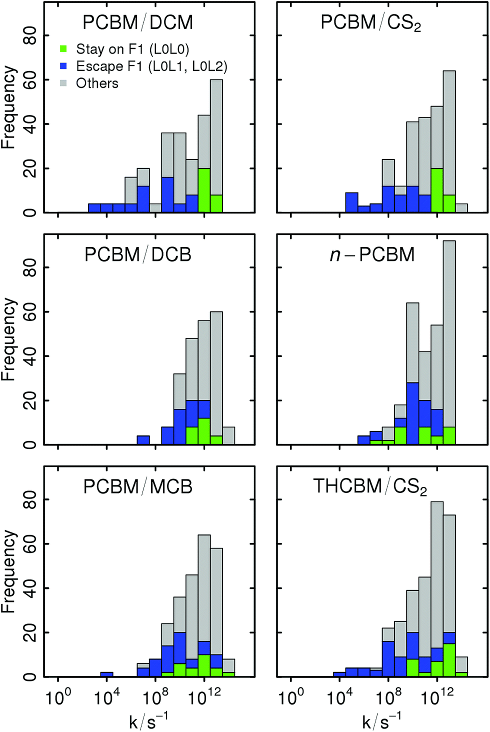 | ||
| Fig. 8 Decomposition of the LZ ET rate distributions of the different crystal structures. Green and blue bins are respectively the contributions of transitions forming the F1-network (L0L0) and those allowing escape from it (L0L1 and L0L2). | ||
4 Summary and conclusions
Progress in organic electronics and photovoltaics requires a thorough understanding of structure–property relationships. These include not just the molecular structure and properties, which from a computational point of view can be now tackled by standard quantum chemical methods, and also supramolecular aspects arising from intermolecular interactions. These are much harder to approach by purely computational methods and, as result, it is almost imperative to combine computational and experimental data on well-defined systems. We have taken such an approach in this study, which has focussed on the relationship between molecular structure, intermolecular packing and electron transport properties for PCBM—currently the most widely used n-type material—and ThCBM—a new, closely related fullerene derivative.We have considered all the available experimental crystal structures of these compounds and applied a hopping model based on a Landau–Zener estimate of the charge transfer rates. Mobility tensors were evaluated by KMC simulations which, in some cases, included the possibility of electron transfer events to/from higher-than-LUMO orbitals. Our results can be summarized as follows:
• PCBM-like molecules may crystallize in different polymorphs forming one-, two- or three-dimensional percolation networks.
• The dimensionality of the electron percolation networks depends on the distribution of the inter-fullerene distances. High electron mobility directions are typically associated with short inter-fullerene distances. For this reason, crystal structures with a short lattice vector display high electron transporting linear channels along that direction.
• The fullerenes' LUMO + 1 and LUMO + 2 orbitals may participate in electron transport. This is especially important for triclinic structures with non-equivalent fullerene molecules as, for example, the LUMO + 1 orbital on one molecule may be degenerate with the LUMO on another. By extrapolation, we expect this “excited state conduction” to be even more important for amorphous structures, where each molecule has a different geometry and environment.
• The highest mobility value has been obtained for a particular direction of the ThCBM/CS2 structure, in which electron transport is highly anisotropic because of perfectly aligned channels presenting high electron transfer rates. We find a mobility of 1.48 cm2 V−1 s−1 associated with that direction which is in good agreement with the experimental mobility value recently reported by Fukuzumi et al. (2.0 cm2 V−1 s−1). ThCBM molecules which dominate charge transport are actually in a low coordination environment (coordination number = 7), while there is a second set of molecules with a higher coordination (10) which make a minor contribution to the mobility.
Further work is currently in progress in order to identify and characterize other crystalline forms of PCBM and new fullerene derivatives.25 The availability of further structural and mobility data on well-defined crystal forms will provide a useful testing ground for current charge transport models. Indeed, there is a real need for new models and computational approaches, overcoming the picture of discrete hopping events among localized electronic states.53,54 Its fundamental inadequacy, which for PCBM already been pointed out by others,27,28 emerges here from the fact that some of our calculated ET rates are comparable with the vibrational frequencies of the fullerene cage (1013 s−1 ≃ 300 cm−1). As a result, the time scale separation assumed by transition-state-type approaches simply does not apply. Suitable extensions of a recently proposed coarse-grained quantum-chemical model of these materials55 may prove to be useful in this context.
Acknowledgements
This work was supported by the Fondazione Cariplo (PLENOS project, ref. 2011-0349) and by Regione Lombardia and CINECA through a LISA supercomputer grant (SIPONS project). We thank Jérôme Cornil and Yoann Olivier from the University of Mons for helpful discussions on the electric field dependency of the electron mobility.References
- J. Hummelen, B. Knight, F. LePeq, F. Wudl, J. Yao and C. A. Wilkins, J. Org. Chem., 1995, 60, 532–538 CrossRef CAS.
- B. C. Thompson and J. M. J. Fréchet, Angew. Chem., Int. Ed., 2008, 47, 58–77 CrossRef CAS PubMed.
- G. Dennler, M. C. Scharber and C. J. Brabec, Adv. Mater., 2009, 21, 1323–1338 CrossRef CAS.
- R. Po, M. Maggini and N. Camaioni, J. Phys. Chem. C, 2010, 114, 695–706 CAS.
- M. T. Dang, L. Hirsch and G. Wantz, Adv. Mater., 2011, 23, 3597–3602 CrossRef CAS.
- F. G. Brunetti, R. Kumar and F. Wudl, J. Mater. Chem., 2010, 20, 2934 RSC.
- A. M. López, A. Mateo-Alonso and M. Prato, J. Mater. Chem., 2011, 21, 1305–1318 RSC.
- J. S. Moore, J. Am. Chem. Soc., 2008, 130, 12201–12203 CrossRef CAS PubMed.
- T. Liu and A. Troisi, Adv. Mater., 2013, 25, 1038–1041 CrossRef CAS PubMed.
- J.-L. Brédas, D. Beljonne, V. Coropceanu and J. Cornil, Chem. Rev., 2004, 104, 4971–5003 CrossRef PubMed.
- K. H. Lee, P. E. Schwenn, A. R. G. Smith, H. Cavaye, P. E. Shaw, M. James, K. B. Krueger, I. R. Gentle, P. Meredith and P. L. Burn, Adv. Mater., 2011, 23, 766–770 CrossRef CAS PubMed.
- N. D. Treat, M. A. Brady, G. Smith, M. F. Toney, E. J. Kramer, C. J. Hawker and M. L. Chabinyc, Adv. Energy Mater., 2011, 1, 82–89 CrossRef CAS.
- J. Zhao, A. Swinnen, G. Van Assche, J. Manca, D. Vanderzande and B. V. Mele, J. Phys. Chem. B, 2009, 113, 1587–1591 CrossRef CAS PubMed.
- C. Müller, T. A. M. Ferenczi, M. Campoy-Quiles, J. M. Frost, D. D. C. Bradley, P. Smith, N. Stingelin-Stutzmann and J. Nelson, Adv. Mater., 2008, 20, 3510–3515 CrossRef.
- X. Yang, J. K. J. van Duren, M. T. Rispens, J. C. Hummelen, R. A. J. Janssen, M. A. J. Michels and J. Loos, Adv. Mater., 2004, 16, 802–806 CrossRef CAS.
- J. Nelson, J. J. Kwiatkowski, J. Kirkpatrick and J. M. Frost, Acc. Chem. Res., 2009, 42, 1768–1778 CrossRef CAS PubMed.
- M. Schrader, R. Fitzner, M. Hein, C. Elschner, B. Baumeier, K. Leo, M. Riede, P. Bäuerle and D. Andrienko, J. Am. Chem. Soc., 2012, 134, 6052–6056 CrossRef CAS PubMed.
- S. Yin, L. Li, Y. Yang and J. R. Reimers, J. Phys. Chem. C, 2012, 116, 14826–14836 CAS.
- F. Frigerio, M. Casalegno, C. Carbonera, T. Nicolini, S. V. Meille and G. Raos, J. Mater. Chem., 2012, 22, 5434–5443 RSC.
- M. T. Rispens, A. Meetsma, R. Rittberger, C. J. Brabec, N. S. Sariciftci and J. C. Hummelen, Chem. Commun., 2003, 2116–2118 RSC.
- N. R. Tummala, S. Mehraeen, Y.-T. Fu, C. Risko and J.-L. Brédas, Adv. Funct. Mater., 2013, 23, 5800–5813 CrossRef CAS.
- M. Casalegno, S. Zanardi, F. Frigerio, R. Po, C. Carbonera, G. Marra, T. Nicolini, G. Raos and S. V. Meille, Chem. Commun., 2013, 49, 4525–4527 RSC.
- G. Paterno, A. J. Warren, J. Spencer, G. Evans, V. G. Sakai, J. Blumberger and F. Cacialli, J. Mater. Chem. C, 2013, 1, 5619–5623 RSC.
- J. H. Choi, T. Honda, S. Seki and S. Fukuzumi, Chem. Commun., 2011, 47, 11213–11215 RSC.
- T. Nicolini and S. V. Meille, in preparation.
- R. C. I. Mackenzie, J. M. Frost and J. Nelson, J. Chem. Phys., 2010, 132, 064904 CrossRef PubMed.
- D. L. Cheung and A. Troisi, J. Phys. Chem. C, 2010, 114, 20479–20488 CAS.
- F. Gajdos, H. Oberhofer, M. Dupuis and J. Blumberger, J. Phys. Chem. Lett., 2013, 4, 1012–1017 CrossRef CAS.
- J. Idé and G. Raos, ChargeTransport: Charge Transfer Rates and Charge Carrier Mobilities, 2014 Search PubMed.
- H. Oberhofer and J. Blumberger, Phys. Chem. Chem. Phys., 2012, 14, 13846–13852 RSC.
- A. B. Bortz, M. H. Kalos and J. L. Lebowitz, J. Comput. Phys., 1975, 17, 10–18 CrossRef.
- R Core Team, R: A Language and Environment for Statistical Computing, R Foundation for Statistical Computing, Vienna, Austria, 2012 Search PubMed.
- B. Baumeier, J. Kirkpatrick and D. Andrienko, Phys. Chem. Chem. Phys., 2010, 12, 11103–11113 RSC.
- E. F. Valeev, V. Coropceanu, D. A. da Silva Filho, S. Salman and J.-L. Brédas, J. Am. Chem. Soc., 2006, 128, 9882–9886 CrossRef CAS PubMed.
- F. Neese, Wiley Interdiscip. Rev.: Comput. Mol. Sci., 2012, 2, 73–78 CrossRef CAS.
- N. M. O'Boyle, A. L. Tenderholt and K. M. Langner, J. Comput. Chem., 2008, 29, 839–845 CrossRef PubMed.
- P.-O. Lowdin, J. Chem. Phys., 1950, 18, 365–375 CrossRef CAS PubMed.
- A. Kubas, F. Hoffmann, A. Heck, H. Oberhofer, M. Elstner and J. Blumberger, J. Chem. Phys., 2014, 140, 104105 CrossRef PubMed.
- E. F. Valeev, V. Coropceanu, D. A. da Silva Filho, S. Salman and J.-L. Brédas, J. Am. Chem. Soc., 2006, 128, 9882–9886 CrossRef CAS PubMed.
- G. D'Avino, S. Mothy, L. Muccioli, C. Zannoni, L. Wang, J. Cornil, D. Beljonne and F. Castet, J. Phys. Chem. C, 2013, 117, 12981–12990 Search PubMed.
- J. Idé, R. Méreau, L. Ducasse, F. Castet, H. Bock, Y. Olivier, J. Cornil, D. Beljonne, G. D'Avino, O. M. Roscioni, L. Muccioli and C. Zannoni, J. Am. Chem. Soc., 2014, 136, 2911–2920 CrossRef PubMed.
- J. E. Norton and J. L. Brédas, J. Am. Chem. Soc., 2008, 130, 12377–12384 CrossRef CAS PubMed.
- D. P. McMahon and A. Troisi, J. Phys. Chem. Lett., 2010, 1, 941–946 CrossRef CAS.
- V. Rühle, A. Lukyanov, F. May, M. Schrader, T. Vehoff, J. Kirkpatrick, B. Baumeier and D. Andrienko, J. Chem. Theory Comput., 2011, 7, 3335–3345 CrossRef PubMed.
- M. Malagoli, V. Coropceanu, D. A. da Silva Filho and J.-L. Brédas, J. Chem. Phys., 2004, 120, 7490–7496 CrossRef CAS PubMed.
- F. Negri and G. Orlandi, J. Chem. Phys., 1995, 103, 2412–2419 CrossRef CAS PubMed.
- D. Fazzi, C. Castiglioni and F. Negri, Phys. Chem. Chem. Phys., 2010, 12, 10–1609 RSC.
- M. J. Frisch, G. W. Trucks, H. B. Schlegel, G. E. Scuseria, M. A. Robb, J. R. Cheeseman, G. Scalmani, V. Barone, B. Mennucci, G. A. Petersson, H. Nakatsuji, M. Caricato, X. Li, H. P. Hratchian, A. F. Izmaylov, J. Bloino, G. Zheng, J. L. Sonnenberg, M. Hada, M. Ehara, K. Toyota, R. Fukuda, J. Hasegawa, M. Ishida, T. Nakajima, Y. Honda, O. Kitao, H. Nakai, T. Vreven, J. A. Montgomery Jr, J. E. Peralta, F. Ogliaro, M. Bearpark, J. J. Heyd, E. Brothers, K. N. Kudin, V. N. Staroverov, R. Kobayashi, J. Normand, K. Raghavachari, A. Rendell, J. C. Burant, S. S. Iyengar, J. Tomasi, M. Cossi, N. Rega, J. M. Millam, M. Klene, J. E. Knox, J. B. Cross, V. Bakken, C. Adamo, J. Jaramillo, R. Gomperts, R. E. Stratmann, O. Yazyev, A. J. Austin, R. Cammi, C. Pomelli, J. W. Ochterski, R. L. Martin, K. Morokuma, V. G. Zakrzewski, G. A. Voth, P. Salvador, J. J. Dannenberg, S. Dapprich, A. D. Daniels, O. Farkas, J. B. Foresman, J. V. Ortiz, J. Cioslowski and D. J. Fox, Gaussian 09, Gaussian, Inc., Wallingford, CT, 2009 Search PubMed.
- J. J. Kwiatkowski, J. M. Frost and J. Nelson, Nano Lett., 2009, 9, 1085–1090 CrossRef CAS PubMed.
- T. Wei, corrplot: Visualization of a correlation matrix, 2013.
- J. Idé, Rpdb: Read, write, visualize and manipulate PDB files, 2014.
- D. Adler, D. Murdoch and others, rgl: 3D visualization device system (OpenGL), 2013.
- S. Stafstrom, Chem. Soc. Rev., 2010, 39, 2484–2499 RSC.
- A. Troisi, Chem. Soc. Rev., 2011, 40, 2347–2358 RSC.
- G. Raos, M. Casalegno and J. Idé, J. Chem. Theory Comput., 2014, 10, 364–372 CrossRef CAS.
Footnotes |
| † Electronic supplementary information (ESI) available: A pdf file containing mathematical derivation of the free energy barriers and rate expressions, numerical data on the Huang–Rhys factors, results for the Marcus and Marcus–Levich–Jortner rate expressions, and a discussion of the electric-field dependence of the mobility. An archive file containing one webGL folder for each crystal structure allowing 3D-visualization (with any HTML5 web browser) of the hopping probabilities derived from the Landau–Zener expression (F3-network). See DOI: 10.1039/c4tc00502c |
| ‡ Present address: Laboratory for Chemistry of Novel Materials, University of Mons, Belgium. |
| This journal is © The Royal Society of Chemistry 2014 |