 Open Access Article
 This Open Access Article is licensed under a Creative Commons Attribution-Non Commercial 3.0 Unported Licence
Measuring the configurational temperature of a binary disc packing
Song-Chuan
Zhao
and
Matthias
Schröter
*
Max Planck Institute for Dynamics and Self-Organization (MPIDS), 37077 Goettingen, Germany. E-mail: matthias.schroeter@ds.mpg.de
First published on 14th March 2014
Abstract
Jammed packings of granular materials differ from systems normally described by statistical mechanics in that they are athermal. In recent years a statistical mechanics of static granular media has emerged where the thermodynamic temperature is replaced by a configurational temperature X which describes how the number of mechanically stable configurations depends on the volume. Four different methods have been suggested to measure X. Three of them are computed from properties of the Voronoi volume distribution, the fourth takes into account the contact number and the global volume fraction. This paper answers two questions using experimental binary disc packings: first we test if the four methods to measure compactivity provide identical results when applied to the same dataset. We find that only two of the methods agree quantitatively. This implies that at least two of the four methods are wrong. Secondly, we test if X is indeed an intensive variable; this becomes true only for samples larger than roughly 200 particles. This result is shown to be due to recently measured correlations between the particle volumes [Zhao et al., Europhys. Lett., 2012, 97, 34004].
1 Is there a well defined configurational temperature?
Temperature is the concept that helps us to understand how the exchange of energy stored in the microscopic degrees of freedom follows from the accompanying change of entropy of the involved systems. If we coarse-grain our view to the macroscopic degrees of freedom of particulate systems, such as foams or granular gases, we can still define effective temperatures that describe their dynamics.1,2 This approach defines these systems as dissipative; the kinetic energy of the particles is irrecoverably lost to microscopic degrees of freedom.In the absence of permanent external driving such a system will always evolve towards a complete rest. In the presence of boundary forces or gravity this rest state will be characterized by permanent contacts between the particles which allow for a mechanical equilibrium. Shahinpoor3 and Kanatani4 were the first to suggest that such systems might still be amenable to a statistical mechanics treatment. Sam Edwards and co-workers5,6 have then developed this idea into a full statistical mechanics of static granular matter by using the ensemble of all mechanically stable states as a basis. A necessary requirement for such an approach is the existence of some type of excitation which lets the system explore the phase space of the possible static configurations. This could e.g. be realized by tapping, cyclic shear, or flow pulses of the interstitial liquid. While there are promising results, the feasibility of this approach is still under debate.7
A second key concept in Edwards' approach is the replacement of the energy phase space by a volume phase space where the volume function W(q) takes the role of the classical Hamiltonian. The configuration q represents the positions and orientations of all grains. One can then define an analog to the partition function Z(X):
 | (1) |
S is neither known from first principles (except for model systems8,9) nor can it be measured directly. Therefore “thermometers” measuring X have to exploit other relationships; four different ways to do so have been suggested. In this paper we will test all four of them using the same dataset of mechanically stable disc packings.
First X can be determined from the steady state volume fluctuations using an analog to the relationship between specific heat and energy fluctuations;10–13 we will refer to this compactivity as XVF. A second method is based on the probability ratio of overlapping volume histograms,14,15 allowing us to compute XOH. A third way16,17 computes XΓ from the Gamma function fits to the volume distribution. Finally, it has been suggested recently18 that an analysis based on so-called quadrons19 instead of Voronoi cells leads to an expression for XQ that involves the average particle volume and the contact number.
This difference in approach immediately raises the question if these four methods provide identical results when applied to the same experiment. There have been two previous experiments addressing this question: McNamara et al.15 found that XVF and XOH agree for tapped packings of approximately 2000 glass spheres. The same result has been reported by Puckett and Daniels20 for compressed disc packings.
A full description of a granular packing has to take the boundary stresses into account.18,21,22 The stress dependence of the entropy then gives rise to a tensorial temperature named angoricity. Angoricity has been computed from numerics using the overlapping histogram method23 and from experiments using both fluctuations and overlapping histograms.20 As the experiments described below are performed in an open cell with gentle driving, the boundary stresses can be assumed to be small and constant; we therefore exclude angoricity from our further analysis.
2 Correlations in the Voronoi-volume of disc packings
The three methods to compute XVF, XOH, and XΓ all start from the Voronoi-volume distribution. However, it has been shown that the Voronoi volumes inside a sample are correlated.25 We recently measured the spatial extension of these correlations and demonstrated the existence of additional anti-correlations between the volumes.24 These correlations raise the question if X is indeed an intensive parameter i.e. if its value is independent of the number N of particles analyzed. As the Voronoi-volumes reported in ref. 24 will be the basis of this study we quickly recap the relevant experimental procedures and results, more details can be found in the original publication. The disc coordinates of all configurations and volume fractions can be downloaded from the Dryad repository.262.1 Experimental setup
The experiment is performed in an air-fluidized bed filled with a binary mixture of Teflon discs with ds = 6 mm and dl = 9 mm diameter. Datasets of 8000 different mechanically stable configurations are prepared by repeated air pulses. Changing pressure and duration of the air pulses allows us to control the average packing fractions ϕ in the ranges of 0.818 to 0.838. After each flow pulse the discs come to a complete rest and are then imaged with a CCD camera (Fig. 1a). After detecting the particle centers, the Voronoi volume V of each disc is determined (Fig. 1b). We then compute the free volume Vf = V − Vmin for each particle with Vmin being the volume the grain would occupy in a hexagonal packing of identical discs. This step allows us to superimpose the results for small and large discs in the subsequent analysis.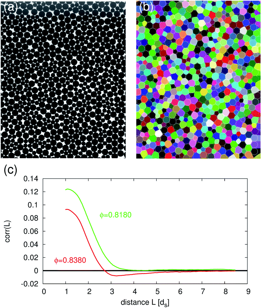 | ||
| Fig. 1 Correlations in binary disc packings. (a) Experimental image and (b) the corresponding Voronoi tessellation. (c) The correlation between two Voronoi volumes as a function of their distance L (measured in units of small disc diameters ds). Dense packings exhibit anti-correlations for L larger than approx. 2.5ds. Reproduced from ref. 24. | ||
Our results will also depend on the packing fraction of the loosest possible packing ϕRLP = 0.811. This value is averaged over 10 packings prepared by slowly settling the discs in a manually decreased air flow.
2.2 Correlations in binary disc packings
The correlation between the Voronoi volumes can be measured using: | (2) |
Here i and j are two points in the packing which are separated by a distance L. The free volumes at these points are Vf,i and Vf,j. Subtracted from them is the average free volume ![[V with combining macron]](https://www.rsc.org/images/entities/i_char_0056_0304.gif) f of all particles at this point (averaged over all 8000 taps). 〈…〉 indicates averaging over the 8000 packings and additionally 240 pairs of points i, j within each packing. σf2 is the variance of the free volumes averaged over the two points.
f of all particles at this point (averaged over all 8000 taps). 〈…〉 indicates averaging over the 8000 packings and additionally 240 pairs of points i, j within each packing. σf2 is the variance of the free volumes averaged over the two points.
Fig. 1c depicts corr(L) for two different packing fractions. At low values of ϕ only positive correlations between Voronoi cells are found. Above ϕAC = 0.8277 anti-correlations appear for L larger than approximately 2.5 small particle diameters. We will show below that these (anti-) correlations control how X becomes intensive.
3 Compactivity XVF measured from volume fluctuations
This methods starts from the assumption of a Boltzmann like probability distribution: | (3) |
From eqn (3) follows the probability to observe a certain volume V at a given compactivity X:
 | (4) |
 counts the number of the mechanical stable states available at volume V. Using eqn (4) we can determine the average volume (X) as
 | (5) |
Taking the derivative of eqn (5) with respect to 1/X shows that
 | (6) |
/d(1/X) can be rewritten as −X2d/dX from which follows: | (7) |
Nowak et al. were the first to suggest that integrating eqn (7) provides a way to compute X:10
 | (8) |
As described in Section 2 we are interested in the evolution of X with the size of the analyzed region, in the following referred to as a cluster. Therefore we continue our study by using the normalized average volume per particle  where the sum goes over all N particles inside the cluster, V is the Voronoi volume of the individual particles and Vg the volume occupied by the particle itself. As a consequence of this choice also X is dimensionless.
Fig. 2a shows that for our tapped disc packings the variance of the volume fluctuation σ![[v with combining macron]](https://www.rsc.org/images/entities/i_char_0076_0304.gif) 2 increases monotonically with the average volume (bar meaning again the average over all 8000 taps). To compute XVF we perform a power law fit to σ2 and use the result to integrate eqn (8) numerically. Fig. 2b shows how the resulting XVF depends on the packing fraction at cluster sizes N of 1, 30, and 150 discs. It is obvious that it is not an intensive variable for this range of N.
2 increases monotonically with the average volume (bar meaning again the average over all 8000 taps). To compute XVF we perform a power law fit to σ2 and use the result to integrate eqn (8) numerically. Fig. 2b shows how the resulting XVF depends on the packing fraction at cluster sizes N of 1, 30, and 150 discs. It is obvious that it is not an intensive variable for this range of N.
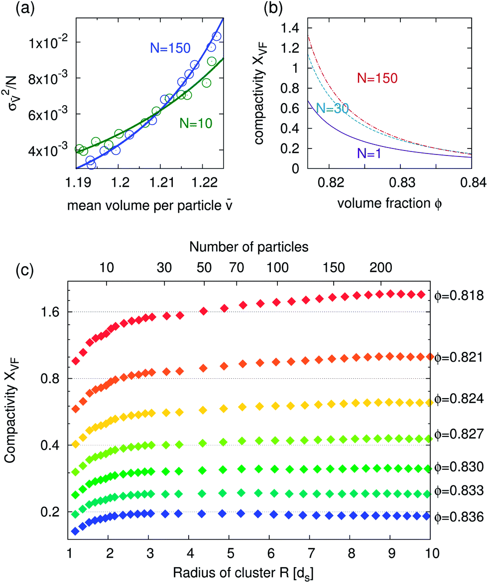 | ||
Fig. 2 Compactivity XVF measured from volume fluctuations. (a) Average volume variance σ2versus average volume measured for clusters of size N = 10 and 150. The solid curves are power law fits which are then used to numerically integrate eqn (8). (b) The compactivity XVF computed from eqn (8) for three different cluster sizes. (c) The evolution of KVF with cluster sizes at different values of ϕ. The radius R of the analyzed cluster is proportional to  . . | ||
3.1 Correlations make XVF non-intensive in small systems
For a more detailed analysis we have plotted in Fig. 2c the dependence of XVF on the cluster radius R measured from small disc diameters ds. Three features of XVF become apparent:(1) XVF is growing monotonously for R < 3ds for all values of ϕ,
(2) for low to intermediate values of ϕ, XVF then reaches a plateau, and
(3) for the highest packing fraction XVF first decreases slightly before entering a plateau.
All three points can be understood by considering the influence of the volume correlations shown in Fig. 1. Eqn (8) computes XVF from the average variance σ2 inside the cluster. This variance can be decomposed in the following way:
 | (9) |
Here σk2 = 〈δvk2〉 is the fluctuation of a single Voronoi cell and  is the volume correlation between disc k and all other discs inside the cluster. If k is in the center of the cluster, then Ik is proportional to the area enclosed by corr(L), the zero line, and L = R in Fig. 1c.
This consideration allows us to explain feature 1: while N goes from 2 to approximately 25 all Ik values are positive and growing. Consequentially, the variance of the cluster σ2 is larger than the sum of the variance of the individual Voronoi cells  and XVF grows monotonously with N.
The second feature stems from the fact that once disk k is more than four to five ds away from the boundary of the cluster, Ik becomes independent of the cluster size. As the relative importance of “boundary discs” decreases with the cluster size, σ2 becomes constant and XVF becomes independent of N.
Finally, the slight decrease in XVF at high packing fractions and N values between approximately 30 and 150 can be attributed to the anti-correlations that appear for ϕ larger than 0.8277; these will decrease Ik slightly again before it reaches its plateau value.
4 Compactivity XOH measured from overlapping histograms
This way to compute compactivity has been first described by Dean and Lefèvre.14 It uses pairs of experiments with slightly different values of ϕ, respectively XOH, and computes then the ratio of the probabilities to observe the same local volume V. If the assumption of a Boltzmann-like probability distribution, as expressed in eqn (4), holds, this ratio should be exponential in V: | (10) |
By taking the logarithm on both sides we obtain:
 | (11) |
Therefore the difference between two compactivities can be computed from a line fit of Q versus V as it was first demonstrated in ref. 15.
Fig. 3a shows the distribution of average volumes for two experiments with a packing fraction difference of 0.0017. Fig. 3b demonstrates that the ratio Q is indeed a linear function of V, as predicted by eqn (11). By sweeping the experimentally accessible range of packing fractions, XOH can be determined from the accumulated compactivity differences up to an additive constant X0. We determine X0 by setting XOH for the loosest experimental packing to the value of XVF at this volume fraction.
 | ||
| Fig. 3 Compactivity measured with the overlapping histogram method. (a) The probability to observe an average volume per particle in clusters with 150 disks. The average packing fraction corresponds to 0.8336 for the red curve, and 0.8353 for the green curve. (b) The logarithm of the probabilities to observe a given volume at two different compactivities respectively packing fractions is a linear function of the volume, which is in accordance with eqn (11). The cluster size is 150 discs, and the dashed lines are linear fits. (c) The χ2 values provide a goodness of fit test for both linear (green diamonds) and parabolic (red triangle) fits to the probability ratios shown in panel b. The average χ2 is 13% smaller for the linear fit, indicating that a Boltzmann-like distribution is a better assumption than a Gaussian. | ||
The resulting XOH is shown in Fig. 4. The good quantitative agreement of XOH and XVF is not too surprising given that (a) both methods are derived from the same probability distribution (eqn (4)) and (b) our determination of X0. However, the XOH method provides an additional test of the assumptions leading to eqn (4) as we can compare the quality of a linear fit to Q(V) with fit functions derived from alternative probability distribution functions.15 A generic candidate would be a Gaussian distribution which results in a parabolic fit. Fig. 3c demonstrates however that a linear fit is superior, adding credibility to a Boltzmann-like approach. Also note that canceling the density of states in eqn (10) implicitly assumes a weak form of ergodicity; if the system explores its phase space differently at the two values of X we cannot eliminate ![[scr D, script letter D]](https://www.rsc.org/images/entities/char_e523.gif) (V).
(V).
 | ||
| Fig. 4 Comparison of XOH, XVF, and XΓ computed for single discs and clusters of 150 particles. In all three cases the compactivity of an individual particle is smaller than that of a larger cluster. XOH and XVF agree quantitatively, XΓ is about an order of magnitude smaller. | ||
5 Compactivity XΓ measured from a Gamma distribution fit
This third method to compute compactivity has been suggested by Aste and Di Matteo;17,27 it differs from the previous approaches that it explicitly determines the density of states(V). Based on the observation16 that experimental Voronoi volume distributions can be well fit by Γ distributions, they propose to replace eqn (4) with a rescaled k-Gamma distribution | (12) |
f is the mean free volume (as defined in Section 2), and k is the shape factor. They then identify | (13) |
f2 of the Γ function is given by: σf2 = f2/k they derive | (14) |
By comparing eqn (4) and (12) we can also identify the density of states:
 | (15) |
Fig. 5a demonstrates that our volume distribution is well fit by a Γ distribution.28 We then determine XΓ without any additive constant using eqn (14). Fig. 4 shows XΓ in comparison to XVF and XOH. While all three compactivities decrease monotonously with ϕ, the absolute values and the slope of XΓ are quite different from XVF and XOH.
 | ||
| Fig. 5 Applying the Γ distribution method. (a) Γ distribution fits to the volume distributions for a single disc and 150 particle clusters (ϕ = 0.8175). (b) Evolution of XΓ with the cluster size. | ||
Fig. 5b shows the evolution of XΓ with the cluster size. A comparison with XVF, displayed in Fig. 2c, shows a qualitative similar influence of the volume correlations: while XΓ increases towards a plateau for small values of ϕ, it goes through a maximum before reaching a smaller plateau value for the densest packings.
6 Compactivity XQ measured from quadron tessellation
In a recent paper Blumenfeld et al.18 presented an analysis of the statistical mechanics of two-dimensional packings based on quadrons19 as the building blocks of the tessellation. An advantage of this choice is that the quadrons take by design into account the structural degrees of freedom of the individual particles. A drawback is that quadrons are not necessarily volume conserving in the presence of non-convex voids formed by “rattlers”, i.e. particles lying at the bottom of larger voids.29,30 Blumenfeld and co-workers then derive the partition functions of the volume ensemble ZV, the force ensemble ZF, and the total partition function Z, showing in this process that Z ≠ ZVZF. Finally, they obtain from Z an expression for XQ of an isostatic packing: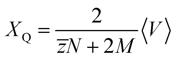 | (16) |
〈V〉 is the average volume of a cluster, ![[z with combining macron]](https://www.rsc.org/images/entities/i_char_007a_0304.gif) the average number of contacts a particle has, and M is the number of boundary forces.
the average number of contacts a particle has, and M is the number of boundary forces.
If XVQ is derived from ZV instead of Z one obtains:
 | (17) |
In comparing our results with this approach we have to acknowledge two differences. First, our experimental packings are clearly subject to volume forces due to gravity. And secondly they are, as shown in Fig. 6a, hyperstatic, i.e. their contact number is larger than what is required to fix all their mechanical degrees of freedom.31
 | ||
| Fig. 6 Compactivity measured with the quadron tessellation method. (a) In all our experiments the contact number per particle is above the isostatic value of 3. (b) A comparison of XQ computed from the full partition function (eqn (16)) and XVQ derived from the volume ensemble (eqn (17)) only. Both are computed for ϕ = 0.8175. The difference vanishes in the large system limit. (c) A comparison of XVF (measured for N = 150) and XVQ. The filled circle is computed for our random loose packing value which is presumably the only isostatic point in our dataset. The open squares assume that eqn (16) is also valid for hyperstatic packings. | ||
Generally, packings of frictional particles only become isostatic at random loose packing and zero pressure.32,33 Therefore the only direct comparison possible is at our RLP value ϕ = 0.811, the corresponding XQ is shown as a black circle in Fig. 6c. If we assume that we can replace in eqn (16) with (ϕ) and use the contact numbers displayed in Fig. 6a, we can also compute XQ for a larger range of ϕ. These results are indicated as open squares in Fig. 6c.
As XQ is only computed from the average volume of a cluster, it is insensitive to the correlations described in Section 2. On the other hand there exists a finite size effect if XVQ is computed from the volume ensemble, ignoring the boundary forces. Fig. 6b shows how the difference between the compactivities computed from the full and the volume ensemble vanishes with increasing cluster size and consequentially decreasing contribution of M.
7 Which is the correct way to measure compactivity?
Fig. 4 and 6c show clearly that the four different methods to compute compactivity do not agree quantitatively. While XOH and XVF are identical within experimental scatter, XΓ is more than one order of magnitude smaller than XOH and XVF and at the same time decreasing less steeply with volume fraction.34 The values of XQ are closer to XOH and XVF again, but the evolution with ϕ is similar to XΓ.Our data can be used to self-consistently compute all four different versions of compactivity, consequentially they are unsuitable as a basis to judge the correctness of the different approaches. A potential experimental or numerical test would need an independent determination of the compactivity of a model system from the knowledge of its entropy as a function of volume. Alternatively, if the granular statistical mechanics could be advanced to make predictions of granular behavior (e.g. segregation35) based on specific values of X, these could be tested versus the four different “thermometers”.
However, we can elucidate the difference between the four methods by computing the density of states and comparing it to what is known about RLP, the loosest possible, mechanically stable packing.
7.1 Computing the density of states
A probability distribution of the type of eqn (3) is a generic feature for every statistic theory that maximizes the amount of entropy represented by p, given certain constraints.36 In this spirit the density of states(V) in eqn (4) can be interpreted as encapsulating the physics of the specific system under consideration, while the exponential term represents our lack of knowledge about the microscopic state. From this perspective the main difference between the four methods is the way they determine (V): while XVF and XOH treat it as an experimental input parameter, XΓ and XQ do provide predictions for its dependence on V. In this subsection we will however not discuss XQ as the theory has not been expanded yet to hyperstatic packings.
(V) can be computed following McNamara et al.15 Starting by rewriting eqn (4) to
| (V) = p(V,X)eV/XZ(X), | (18) |
 | (19) |
The results are presented in Fig. 7 where we have chosen V0 = 1.2. Panel (a) shows that the density of state ratios computed from all eleven values of XOH overlap, as it can be expected if the different preparation protocols sample the phase space with the same probabilities. Fig. 7b shows that this agreement of the density of states is not obtained if the ratio is computed from XΓ.
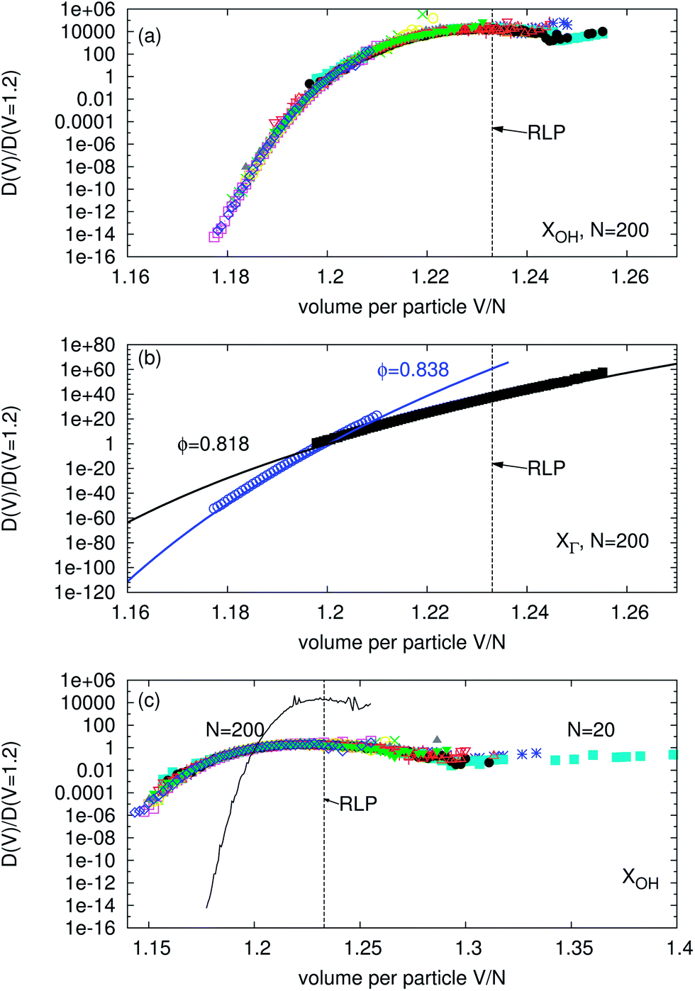 | ||
| Fig. 7 The density of states ratio. Panel (a) is based on the eleven measurements of XOH for the cluster size N = 200. The dashed line indicates the global random loose packing volume. Panel (b) is computed from XΓ of the densest and loosest packings. Points represent the measured distributions, solid lines are analytical results based on the Gamma functions (eqn (15)). In contrast to panel (a) the two curves do not overlap. (c) The density of states depends on the cluster size. The solid, black curve corresponds to the average of all data points with N = 200 in panel (a), the individual data points are computed from XOH measured at N = 20. | ||
Fig. 7 provides also some insight into how the configurational entropy S depends on the volume:
S = kE![[thin space (1/6-em)]](https://www.rsc.org/images/entities/char_2009.gif) ln((V)δV) = kEln(V) + kElnδV ln((V)δV) = kEln(V) + kElnδV | (20) |
(V) and can therefore choose the integration interval δV small enough so that its contribution to S vanishes.
7.2 Random loose packing
Random Loose Packing (RLP) is first of all defined phenomenologically as the loosest possible packing which is still mechanically stable, i.e. has a finite yield stress. Mechanical stability requires the packing to be at least isostatic: the average number of contacts of a particle needs to be large enough to provide sufficient constraints to fix all its degrees of freedom.32,33,38 Experimentally it has been found that ϕRLP of spheres is approximately 0.55 (ref. 39–42) with the precise value depending on the friction coefficient μ (ref. 40–42) and the confining pressure.40 For binary disc packings ϕRLP also depends on their diameter ratio; for the particles in this paper we measured ϕRLP = 0.811.While RLP seems to imply that there exist no packings with lower ϕ, exactly such states have been identified in MD simulations with N = 20 discs; the new lower boundary where such states vanish has been named Random Very Loose Packing (RVLP).43 An explanation why these states between RLP and RVLP are usually not observed in experiments is given by their small basin of attraction in phase space.
In general, the statistical mechanics approaches to granular media5–7 assume the configurational temperature X ≥ 0. Then it follows from
| ∂S = 1/X∂V | (21) |
The density of states computed from XVF, respectively XOH, agrees with these predictions; Fig. 7 shows that it reaches a global maximum at RLP. This is however only a self-consistency test as the value of ϕRLP explicitly entered the computation of these two compactivities. More probative is the fact that the volume fluctuations used to compute XVF have been shown to depend on μ.11 Consequentially, also a configurational entropy computed from XVF will depend on μ, which is a necessary condition as the number of mechanically stable configurations also depends on μ.
Fig. 7c shows that the density of states also depends on the size of the system. Systems with 20 discs posses considerably looser states than those with 200 discs. This effect points to an explanation of the configurations between RLP and RVLP as a consequence of the finite size of a system, they will vanish in the thermodynamic limit.
The density of states computed from XΓ (Fig. 7b) seems not to display a maximum at ϕRLP. However, RLP might become the most likely state if in the limit N → ∞ the states between RLP and RVLP vanish. Either way, XΓ(ϕRLP) will be finite and display a jump to approximately half its value for the “fluid” configurations below ϕRLP,27 which have Voronoi volume distributions that are also well described by Gamma functions.44 While this behavior might be not the canonical expectation, especially as XΓ is undefined for fluid, non-stable configurations, it does not contradict experimental results. This is different for the influence of friction: it has been shown that the Gamma distribution fits are independent of μ,16,17 consequentially neither ϕRLP nor XΓ and the derived S will reflect the different number of mechanical stable states resulting from changes in friction.
Finally, it is difficult to comment on the relationship between XQ and RLP as the theory is presently only worked out at exactly RLP. XQ (ϕRLP) is of finite value and will depend only very weakly on μ via V. If we allow similar to XΓ for its existence also for ϕ < ϕRLP, XQ will be depending on the preparation protocol because the contact number is protocol dependent below RLP.45
7.3 Open questions
Because granular matter is athermal, the question of ergodicity has to be answered separately for each experimental or numerical protocol used to explore the phase space of mechanically stable configurations. An indication of their differences is e.g. the different ϕ dependence of the volume fluctuations when the sample is either mechanically tapped12 or excited by flow pulses.11 Nonergodicity has recently also been shown for numerical tapping of frictionless hard spheres,46 however there the analysis was not restricted to mechanically stable states. In contrast, in numerical simulations of frictional discs fluidized with flow pulses an equivalence between time and ensemble averages has been found.47The biggest challenges to the concept of a configurational granular temperature are however recent experiments by Puckett and Daniels20 where they studied the volume and force fluctuations of two samples of discs which where in mechanical contact. They found that the angoricity of the two samples equilibrated, but the compactivity (computed as XOH and XVF) did not. However, their preparation protocol was biaxial compression which did not allow for strong particle rearrangements. Therefore, we speculate, it might have been prohibiting volume exchange between the two subsystems by quenching too fast. Clearly more work is needed to answer the question if compactivity is a variable predictive of granular behavior or just a number following from an algorithm.
8 Conclusions
Using the same experimental dataset, we have computed the configurational granular temperature X with the four different methods that have been previously suggested. The two methods that treat the density of states as an experimental input agree quantitatively with each other. The X values computed from the other two methods, which specify the density of states from independent theoretical considerations, are both different from each other and from the first two methods. Our results do not provide a direct way to judge the correctness of the individual approaches. But the derived density of states shows that only the two agreeing methods provide a satisfying explanation how random loose packing depends on friction.Our measurements also demonstrate that X becomes only an intensive variable when computed for clusters of size N larger 150 particles. This effect is due to the volume correlations of neighboring particles. Consequentially, individual Voronoi cells are not suitable ‘quasi-particles’ to define a configurational temperature in granular packings. This will complicate the application of a statistical mechanics approach to small granular systems and in the presence of local gradients.
Acknowledgements
We acknowledge helpful discussions with Karen Daniels and Klaus Kassner.References
- I. K. Ono, C. S. OHern, D. J. Durian, S. A. Langer, A. J. Liu and S. R. Nagel, Phys. Rev. Lett., 2002, 89, 095703 CrossRef PubMed.
- N. V. Brilliantov and T. Pöschel, Kinetic Theory of Granular Gases, Oxford University Press, 2004 Search PubMed.
- M. Shahinpoor, Powder Technol., 1980, 25, 163–176 CrossRef.
- K.-I. Kanatani, Powder Technol., 1981, 30, 217–223 CrossRef.
- S. Edwards and R. Oakeshott, Phys. A, 1989, 157, 1080–1090 CrossRef.
- A. Mehta and S. F. Edwards, Phys. A, 1989, 157, 1091–1100 CrossRef.
- M. Pica Ciamarra, P. Richard, M. Schröter and B. P. Tighe, Soft Matter, 2012, 8, 9731 RSC.
- R. Monasson and O. Pouliquen, Phys. A, 1997, 236, 395–410 CrossRef.
- R. K. Bowles and S. S. Ashwin, Phys. Rev. E: Stat., Nonlinear, Soft Matter Phys., 2011, 83, 031302 CrossRef.
- E. R. Nowak, J. B. Knight, E. Ben-Naim, H. M. Jaeger and S. R. Nagel, Phys. Rev. E: Stat., Nonlinear, Soft Matter Phys., 1998, 57, 1971–1982 CrossRef CAS.
- M. Schröter, D. I. Goldman and H. L. Swinney, Phys. Rev. E: Stat., Nonlinear, Soft Matter Phys., 2005, 71, 030301 CrossRef.
- P. Ribière, P. Richard, P. Philippe, D. Bideau and R. Delannay, Eur. Phys. J. E: Soft Matter Biol. Phys., 2007, 22, 249–253 CrossRef PubMed.
- C. Briscoe, C. Song, P. Wang and H. A. Makse, Phys. Rev. Lett., 2008, 101, 188001–188004 CrossRef PubMed.
- D. S. Dean and A. Lefèvre, Phys. Rev. Lett., 2003, 90, 198301 CrossRef PubMed.
- S. McNamara, P. Richard, S. K. de Richter, G. Le Car and R. Delannay, Phys. Rev. E: Stat., Nonlinear, Soft Matter Phys., 2009, 80, 031301 CrossRef.
- T. Aste, T. D. Matteo, M. Saadatfar, T. J. Senden, M. Schröter and H. L. Swinney, EPL, 2007, 79, 24003 CrossRef.
- T. Aste and T. Di Matteo, Phys. Rev. E: Stat., Nonlinear, Soft Matter Phys., 2008, 77, 021309 CrossRef CAS.
- R. Blumenfeld, J. F. Jordan and S. F. Edwards, Phys. Rev. Lett., 2012, 109, 238001 CrossRef PubMed.
- R. Blumenfeld and S. F. Edwards, Phys. Rev. Lett., 2003, 90, 114303 CrossRef PubMed.
- J. G. Puckett and K. E. Daniels, Phys. Rev. Lett., 2013, 110, 058001 CrossRef PubMed.
- K. Wang, C. Song, P. Wang and H. A. Makse, Europhys. Lett., 2010, 91, 68001 CrossRef.
- L. A. Pugnaloni, J. Damas, I. Zuriguel and D. Maza, Pap. Phys., 2011, 3, 030004 Search PubMed.
- S. Henkes, C. S. O'Hern and B. Chakraborty, Phys. Rev. Lett., 2007, 99, 038002 CrossRef PubMed.
- S. Zhao, S. Sidle, H. L. Swinney and M. Schröter, EPL, 2012, 97, 34004 CrossRef.
- F. Lechenault, F. d. Cruz, O. Dauchot and E. Bertin, J. Stat. Mech.: Theory Exp., 2006, 2006, P07009 Search PubMed.
- Data available from the Dryad Digital Repository: http://doi.org/10.5061/dryad.t6m37.
- T. Aste and T. Di Matteo, Eur. Phys. J. B, 2008, 64, 511–517 CrossRef CAS.
- The theory leading to XΓ has been developed for three-dimensional monodisperse packings. Our approach of using binary two-dimensional data is justified only empirically by the quality of the Gamma distribution fit (i.e. eqn (12)) to our free volume distribution.
- M. Pica Ciamarra, Phys. Rev. Lett., 2007, 99, 089401 CrossRef.
- R. Blumenfeld and S. F. Edwards, Phys. Rev. Lett., 2007, 99, 089402 CrossRef.
- Two particles are considered to be in contact when the distance between their centers is smaller than 1.01 times the sum of their radii. The prefactor is based on the uncertainty of our image processing, it has been measured from the pair correlation function.
- K. Shundyak, M. van Hecke and W. van Saarloos, Phys. Rev. E., 2007, 75, 010301 CrossRef.
- S. Henkes, M. van Hecke and W. van Saarloos, EPL, 2010, 90, 14003 CrossRef.
- This difference can not be attributed to the use of the free volume Vf for the computation of XΓ as Vf differs from v only by a constant
 . Therefore neither the shape of the probability distributions used to compute XOH nor the size of the volume fluctuations, on which XVF is based on, would change if they were also computed from Vf.
 - M. Schröter and K. E. Daniels, arxiv.org/abs/1206.4101.
- E. T. Jaynes, Phys. Rev., 1957, 106, 620–630 CrossRef.
- G.-J. Gao, J. Bławzdziewicz and C. S. O'Hern, Phys. Rev. E: Stat., Nonlinear, Soft Matter Phys., 2006, 74, 061304 CrossRef.
- C. Song, P. Wang and H. A. Makse, Nature, 2008, 453, 629–632 CrossRef CAS PubMed.
- G. Y. Onoda and E. G. Liniger, Phys. Rev. Lett., 1990, 64, 2727–2730 CrossRef CAS PubMed.
- M. Jerkins, M. Schröter, H. L. Swinney, T. J. Senden, M. Saadatfar and T. Aste, Phys. Rev. Lett., 2008, 101, 018301 CrossRef PubMed.
- G. R. Farrell, K. M. Martini and N. Menon, Soft Matter, 2010, 6, 2925–2930 RSC.
- L. E. Silbert, Soft Matter, 2010, 6, 2918–2924 RSC.
- M. Pica Ciamarra and A. Coniglio, Phys. Rev. Lett., 2008, 101, 128001 CrossRef.
- V. Senthil Kumar and V. Kumaran, J. Chem. Phys., 2005, 123, 114501 CrossRef.
- C. Heussinger and J.-L. Barrat, Phys. Rev. Lett., 2009, 102, 218303 CrossRef PubMed.
- F. Paillusson and D. Frenkel, Phys. Rev. Lett., 2012, 109, 208001 CrossRef PubMed.
- M. Pica Ciamarra, A. Coniglio and M. Nicodemi, Phys. Rev. Lett., 2006, 97, 158001 CrossRef PubMed.

| This journal is © The Royal Society of Chemistry 2014 |