A coarse-grained molecular dynamics – reactive Monte Carlo approach to simulate hyperbranched polycondensation

Abstract

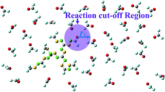
A coarse-grained molecular dynamics (CG-MD) and reactive Monte Carlo (RMC) hybrid method (CG-MD + RMC) has been developed to investigate the hyperbranched polycondensation of 3,5-bis(trimethylsiloxy)benzoyl chloride to poly(3,5-dihydroxybenzoic acid). The CG force field to describe the formation of the hyperbranched macromolecules has been extracted from all-atom molecular dynamics simulations by the mapping technology of iterative Boltzmann inversion. In the mapping process branched poly(3,5-dihydroxybenzoic acid) in an all-atom description has been employed as a target object to derive the CG force field for hyperbranched polymers. In the RMC simulations, the reactivity ratio of the functional groups has been optimized by fitting experimental data with the iterative dichotomy method (Macromolecules, 2003, 36, 97). Using such a simulation framework, detailed information including the molecular weight, the molecular weight distribution and the branching degree of a specific polymerization process has been derived. Radial distribution functions of the atomistic and coarse-grained systems are in excellent agreement. A good agreement between the present simulations and experiment has been demonstrated, too. Especially, the intramolecular cyclization fraction has been reproduced quantitatively. This work illustrates that the present reactive CG-MD + RMC model can be used for quantitative studies of specific hyperbranched polymerizations.

---

1 Introduction

As multifunctional materials, hyperbranched polymers have drawn much attention in the fields of drug carriers, biomaterials, catalysts, coatings and polymer electrolytes. On the one hand, this is caused by their multi-modifiable terminal groups, on the other by their unique properties such as high solubility and low viscosity.^1,2 Various hyperbranched polymers including polyesters, polyethers, polyimides and polyphenylenes could be synthesized by simple one-pot polymerizations.^3–6 At present, however, the characterization of hyperbranched polymers at a molecular scale is still difficult due to their complex and disordered structures which not only depend on the monomer components but also on details of the synthetic route. Quantitative understanding of the polymerization kinetics and the structure of these complex macromolecules is important when trying to improve and to control their building principles and properties.

In the past, a variety of theoretical and simulation methods such as mean-field based kinetic models,^7–13 lattice and off-lattice Monte Carlo (MC) models^14–18 were developed to explore the reaction kinetics and structural properties of hyperbranched polymers. They have been studied with and without the consideration of properties such as steric effects, the relaxation of polymer chains and intramolecular cyclizations. Most previous efforts were focused on the generic properties of hyperbranched polymerizations. These approaches covered the influence of substitutions,^9,12,18–21 the addition of core molecules,^11,22–25 intramolecular ring units,^14,17,26,27 the monomer concentration,^17,21,28 and the chain rigidity as well as the reaction reversibility²⁹ on the molecular weight distribution and degree of branching. To our knowledge, investigations of specific hyperbranched polymerizations using a molecular model with structural details have been reported neither in theoretical nor in simulation studies.^30–32 Such techniques, however, are the prerequisite to understand specific hyperbranched polymerizations quantitatively.

In contrast to generic theoretical methods, molecular dynamics (MD) simulations can describe specific systems under realistic conditions. The recently developed reactive molecular dynamics (RMD) methods are a feasible way to explore complex reactive systems. In RMD approaches, chemical reactions are introduced into a classical model.³³ Thus one has to restrict such simulations to reactive processes where (nuclear) quantum effects can be neglected. In recent Feynman path-integral Monte Carlo studies, it had been shown that (intramolecular) reactions of non-hydrogen atoms can be described adequately in a classical approximation for temperatures ≥298 K.^34,35 In rearrangement processes of hydrogen atoms, quantum fluctuations are non-negligible in the vicinity of (and even below) room-temperature. The heavy coarse-grained beads, see below, in the present reactive approach imply that a classical approximation should be sufficient. If this is guaranteed the predictive capability of RMD and conventional MD simulations strongly depends on the accuracy of the force field. Some works using generic potentials without molecular details^36–38 studied cross-linking reactions and phase separations induced by polymerization processes.^39–42 The more accurate but complex atomistic force fields including RMDff,⁴³ REBO,⁴⁴ AIREBO⁴⁵ and ReaxFF⁴⁶ were developed with the intention to simulate degradation and decomposition reactions of polymers and energetic materials,^47–54 formation processes and properties of carbon systems,^{46, 55–60} as well as transition metal catalyzed reactions.^61,62 The merits of these reactive force fields have been summarized in a recent state of the art description.³³ Review articles on earlier reactive MD methods and the force fields employed in these studies had been published before.^63,64

It is well known that simple generic potentials cannot be used to study specific systems, although they are useful to derive general trends as a function of a chosen grid of parameters. Realistic potentials from, e.g., quantum chemistry calculations⁶⁵ in atomistic resolution, however, require extensive computational capacities when calculating large systems. In order to enhance the efficiency in the simulation of specific systems, coarse-graining (CG) techniques^66,67 have been proposed in MD and MC studies. Among other applications such CG simulations have been employed in studies of biological and soft matter systems.^67–71 In a CG picture, several atoms of the atomistic system are grouped together to so-called superatoms or CG beads. As a matter of fact, CG force fields combine the advantages of generic and atomistic simulations but avoid their shortcomings. On the one hand, they reproduce certain characteristics of the systems (e.g. structural,^72–75 thermodynamic^68,76 or dynamic properties^69,77), on the other, they improve the computational efficiency to a great extent. CG force fields have been applied recently to study polymerization reactions of specific molecules. For example, Farah et al. analyzed the living polymerization of styrene⁷⁸ and cross-linking reactions near selective surfaces.⁷⁹ The adopted CG force fields were developed by iterative Boltzmann inversion (IBI) with the aim to reproduce the molecular structures.⁷⁵ Liu et al.⁸⁰ studied the formation mechanism of a typical epoxy resin on carbon fibres by using reactive dissipative particle dynamics (DPD).^81,82 Preceding atomistic MD simulations have been performed to determine the parameters required in the DPD simulations. The computational capability of RMD methods equipped with an accurate CG force field has been demonstrated recently in a study analyzing the curing of bifunctional epoxies with pentafunctional amines in the neighborhood of a surface allowing amine adsorption.⁸³ More information on reactive MD techniques can be found in the review articles mentioned above.^33,63,64

In the present work, we develop a reactive coarse-grained model by hybridizing molecular dynamics and reactive Monte Carlo methods (CG-MD + RMC) to study a specific hyperbranched polymerization quantitatively. A capture radius criterion similar to the work of Farah et al.³³ has been employed in our study to initiate and control chemical reactions. In contrast to past simulation approaches,^{33,36–38,78} several refinements have been considered in the present reactive model. Thus the probability of a reaction is correlated with the structure of the reacting molecules. With this improved model, we simulate the polyesterification of bulk 3,5-bis(trimethyl-siloxy)benzoyl chloride (BTMSBCl) (Fig. 1a) to yield hyperbranched poly(3,5-dihydroxybenzoic acid) (PBTMSBCl) (Fig. 1b). This polyester is one of the earliest prepared hyperbranched polymers which is formed by AB₂ type monomers.^5,30,84 Note that A, B denote CG beads in the studied systems. The reaction kinetics is still not fully understood although it has been studied both in experiments and in the framework of a mean-field theory.³⁰ In our simulations, the chosen reaction temperature (T) of 443 K is the same as in experiment.³⁰ BTMSBCl has been used as the reactive monomer to retain typical characteristics of hyperbranched polyester units. The substitution effect (i.e. the influence of an electron-donating or electron-withdrawing group on a reactive step) is represented by a reactivity ratio for the coarse-grained functional groups. In the present work, a “functional group” characterizes a subunit (i.e. a bead in the CG picture) in the monomer or polymer; see Fig. 1 for a graphical representation. We have used experimental data (ratios or mole fractions of structural units, conversion rates of functional groups)³⁰ to optimize the reactivity ratios. With our model, quantitative information on the degree of polymerization, the polydispersity index, the degree of branching and intramolecular cyclization can be obtained. Radial distribution functions calculated in the atomistic and coarse-grained systems have been compared by using a reverse mapping technique.^85–87 The present simulations are also correlated with experimental results.

Fig. 1 Coarse-grained mapping scheme of 3,5-bis(trimethylsiloxy)benzoyl chloride (a) and branched poly(3,5-bis(trimethylsiloxy)benzoyl chloride) (b). TMSO (OTMS) stands for the trimethylsiloxy fragment. The symbols A, B and C characterize coarse-grained superatoms in the monomer and polymer units which are labeled by the capital letters M and P. In the polymer the unreacted A and B functions, i.e. PA and PB, have to be discriminated from their reacted counterparts Pa and Pb.

2 Development of the coarse-grained force field

In experiments the 3,5-bis(trimethylsiloxy)benzoyl chloride monomer BTMSBCl is polymerized to the hyperbranched polymer PBTMSBCl. The CG force fields of the monomers and polymers have been developed for the bulk systems of monomeric 3,5-bis(trimethylsiloxy)benzoyl chloride (BTMSBCl) (Fig. 1a) and branched polymeric poly(3,5-bis(trimethylsiloxy)benzoyl chloride) (PBTMSBCl) (Fig. 1b). The polymers formed are poly(3,5-dihydroxybenzoic acid) oligomers saturated at its unreacted sites with residual –OSiMe₃ (at –OH sites) and –COCl (at –COOH sites) groups (Fig. 1b). The molecular dynamics simulations of the atomistic and coarse-grained systems have been carried out by using the open software code GROMACS 4.5.⁸⁸ The mapping procedure and details in developing the CG force fields are described in the following subsections.

2.1 Details of atomistic molecular dynamics simulations

In the atomistic molecular dynamics simulations, the bulk systems of BTMSBCl (Fig. 1a) and PBTMSBCl (Fig. 1b) including the force field used (GROMOS96 53a6) and the initial partial charges are constructed by the program PRODRG.⁸⁹ For the monomer system we have used 1000 BTMSBCl molecules in a cubic simulation box. In the polymer system, 167 branched PBTMSBCl hexamers have been chosen to keep the number of units similar to the bulk system of monomers. Neither the monomer system nor the polymer system contains a solvent. First, isothermal–isobaric (NPT) simulations of the BTMSBCl bulk system have been performed to fix the size of the simulation space. In the NPT calculations, the GROMOS96 53a6 force field⁹⁰ has been applied. In analogy to experiment the simulations have been performed at a temperature of 443 K and a pressure of 101.3 kPa. The integration time step is 0.002 ps; the bonds with the H atoms are constrained.⁹¹ The cutoff values of the nonbonded van der Waals interactions are 1.0 nm. The electrostatic interactions are calculated using the particle mesh Ewald method.⁹² At first, the system of BTMSBCl monomers was equilibrated in the NPT ensemble for 1.0 ns using the Berendsen coupling method for the temperature (coupling time 0.3 ps) and pressure (coupling time 3.0 ps). In the second step, another NPT simulation (only for the BTMSBCl system) of 1.0 ns has been performed with a Nose–Hoover thermostat (coupling time 0.3 ps) and a Parrinello-Rahman barostat (coupling time 3.0 ps) to calculate the volume of the system. After the volume fluctuated around a constant value, the average volume at equilibrium has been calculated as 502.5 nm³ leading to a side length of the cubic box of 7.95 nm and an average density of 1033 kg m⁻³ (see ESI, S1†). Finally, atomistic MD simulations of the monomer system BTMSBCl and the branched PBTMSBCl polymer have been performed for a long time (10 ns) in the NVT ensemble (T = 443 K, cubic simulation cell with side length L = 7.95 nm) under conservation of all other parameters.

2.2 Mapping scheme

In the mapping from the atomistic to the coarse-grained structure, each BTMSBCl monomer has been coarse-grained to four CG beads, i.e. one A function, two B functions and one linking C function (see Fig. 1). The capital letters M and P in the diagrams discriminate between monomer (Fig. 1a) and polymer (Fig. 1b) units. In the monomer (BTMSBCl), the –COCl, –(C₆H₃), and –OTMS groups are mapped by the CG particles MA, MC and MB. In branched PBTMSBCl, the –COCl, –CO–, –(C₆H₃), –OTMS and –O– groups form the set of CG particles PA, Pa, PC, PB and Pb. The symbols in the text and in Fig. 1 with a lowercase letter refer to CG beads after a reaction, while the labels with a capital letter denote unreacted beads. In the atomistic model, polymerization proceeds via formation of a new C–O bond by condensation. In the CG representation, a reactive step involves a transition from MA (PA) and MB (PB) beads to Pa and Pb beads. Table 1 shows the correlation between the employed CG beads and the chemical groups in atomistic resolution. The scheme helps to identify the chemical reaction studied in the present contribution. The CG particles are centered on the C atom in the case of the –COCl and –CO– groups, on the geometric center of the atoms for the –(C₆H₃) and –OTMS groups, and on the O atom for the –O– groups. In the present coarse-grained simulations of polymers, nonbonded interactions have been excluded for first and second neighbour particles.

Table 1 Correlation between the employed CG beads in the monomer (M) and polymer (P) units and the chemical groups in atomistic resolution. In the hyperbranched polymer, the reacted and unreacted groups have to be discriminated

Monomer		Polymer, unreacted		Polymer, reacted
MA	–COCl	PA	–COCl	Pa	–CO–
MB	–OSiMe3	PB	–OSiMe3	Pb	–O–
MC	–C6H3	PC	–C6H3

---

2.3 Coarse-grained force fields of monomers and polymers

The coarse-grained MD simulations of both BTMSBCl and branched PBTMSBCl have been performed under NVT conditions at T = 443 K with the Nose–Hoover thermostat (coupling time 0.3 ps). In the coarse-grained MD, the CG particles are uncharged, the electrostatic interactions are considered implicitly through the IBI mapping of the atomistic system;⁷⁵ the nonbonded interactions are truncated at a distance of 1.5 nm. The time step equals 0.005 ps and each system runs for 1.0 ns.

The total interaction potential of the coarse-grained system (U_total) is composed of the bonded (U_bond) and nonbonded potential (U_nb).

U_total = U_bond + U_nb (1)

The bonded potential includes three elements, i.e. the bond (U_bo), angle (U_an) and improper dihedral potential (U_im). The improper dihedral in this work allows to conserve a planar structure of the four CG particles of a monomeric unit.

U_bond = U_bo + U_an + U_im (2)

In our CG model, the bonded potentials are either given analytically in the harmonic approximation or provided in tabulated form. Most bonded interactions can be described as harmonic form; for the complex target angle distributions involving the –OTMS function, the tabulated form is required. The tabulated form is also used for the nonbonded (nb) potential. The initial values bo₀, an₀, im₀ of the CG parameters for the harmonic potentials (eqn (3)) and the tabulated potentials (eqn (4)) can be calculated by simple Boltzmann inversion of distribution functions (p_bo, p_an, p_im) obtained from atomistic reference simulations. The symbols bo, an and im denote the actual values of bondlength, angle and improper dihedral angle.

U_nb = −k_BT ln g(r) (4)

In the last equation g(r) is the radial distribution function (rdf). k_B is the Boltzmann constant. The rdfs have been measured with respect to the bead center which has been explained at the end of Section 2.2.

In the definition of the CG force fields, the tabulated potentials have been fixed initially when optimizing the parameters of the harmonic interactions. The spring constants (k_bo, k_an, k_im) and the structural equilibrium values (bo₀, an₀, im₀) in eqn (3) have been tuned iteratively until the target (t) distributions of bonds, angles and improper dihedrals were fitted with sufficient accuracy. After that, the harmonic potential has been fixed and the tabulated potential has been optimized using iterative Boltzmann inversion (IBI).⁷⁴

The values U_x,i+1(r) and U_x,i(r) in eqn (5) (with x = an, nb) symbolize the potential in the (i + 1)th and ith iteration step, f and ν are two small parameters to tune the correction term in each iteration step. p_an,i and g_i(r) symbolize the angle and radial distribution functions in the ith iteration while p_an,target and g_target(r) stand for the target p_an and g(r) from an atomistic simulation. The final distribution functions for BTMSBCl and branched PBTMSBCl that have been derived on the basis of the optimized CG force fields, are shown in the ESI, SF4–SF7.† The agreement between CG and atomistic reference distributions is very good. The parameters of the harmonic potential of BTMSBCl and PBTMSBCl are shown in S2 and S3.† The tabulated force fields are provided in the supporting files, too.

For the polymerized system with its monomeric units and polymer chains, the interaction potential between the components is required. We use the arithmetic mean of the interactions between identical components (eqn (6)).

U_M and U_P represent the nonbonded interaction potentials between the monomers (BTMSBCl) and between polymer units (PBTMSBCl), respectively. The distribution functions of both resolutions at all conversions of A function, c_A, have been checked to make sure that the present coarse-grained model is suitable. It can be seen in Fig. 2 that all radial distribution functions agree well in their peak positions. There are only small differences in their peak intensities which are enlarged with increasing c_A (Fig. 2, lower right diagram). Thus it can be assumed that the above model assumptions and the combination rule applied in developing the CG force fields are a reasonable strategy to simulate hyperbranched polymerizations (specific radial distribution functions of A, B and C functions can be found in S8.†). In order to compare the diffusion behaviours of atomistic and CG models, the diffusion constants, D_M and D_P in the atomistic and CG models (here, M and P stand for monomer and branched polymer, respectively, see Fig. 1) have been calculated. The values of D_M equal 539.7 and 3806.5 μm² s⁻¹ for the atomistic and CG model, respectively. For the polymer, D_P equals 30.9 and 1001.5 μm² s⁻¹ for atomistic MD and CG-MD, respectively. The diffusion of CG molecules is much faster than atomistic molecules. Although polymerizations are kinetic processes the difference in the diffusion coefficient between atomistic and CG approaches causes no problem as the simulation time scale is not related to the experimental time scale.

Fig. 2 Calculated nonbonded radial distribution functions of all particles, g(r), from fully atomistic and coarse-grained simulations at different conversions of A functions, c_A.

3 Model and simulation details

3.1 Simulation procedure and computational conditions

In this work, a coarse-grained reactive model combining molecular dynamics and reactive Monte Carlo methods has been developed to study AB₂ type hyperbranched polymerizations. Similar to former RMD studies,^{37,38,78–80} a capture radius, r_c, has been employed to steer the reactive processes. The parameter r_c is set to 0.5 nm according to the position of the first peak of the nonbonded distribution function curve for MA and MB (see picture (d) in ESI, S5†). In an attempted reaction, an active center (an unreacted A function or an unreacted B function) is first determined randomly. Then, the closest unreacted complementary particle within the capture radius r_c of the active center, is selected as a candidate for a reaction. It is assumed that the local equilibrium for each molecular conformation is always reached at coarse-grained reaction time. The reaction can be controlled by a probability parameter P_r. If the two particles do not belong to the same unit, a random number γ ∈ [0,1] is generated to decide whether the reaction takes place. When γ < P_r, the reaction occurs, the interaction parameters of the connected particles are switched from a nonbonded to a bonded state and the type of the reacted particles changes. The factor P_r is the critical parameter which allows to tune the relative reactivity of functional groups. In an AB₂ type hyperbranched polymerization, P_r is expressed by three “reactivity parameters” r_i (i ∈ {B, b, A, a, BB, Bb, bb}) which are given in eqn (7). In a reaction cut-off region, the reactive process between two monomer (polymer) units occurs in a way, as illustrated in Table 2. The units in the top row have an active A function which is underlined. The remaining two B or b (unreacted or reacted) functions may influence the reactivity of the A function by means of the reactivity parameter r_BB/Bb/bb. The slash symbol between the lower indices of the r-symbol means “or”. There are three reactivity parameter combinations when the reactive group is the A function. At first we can have two unreacted B functions symbolized by the reactivity parameter r_BB. The second one refers to one unreacted B function and one reacted B function (=b) which is mapped by the reactivity parameter is r_Bb. Finally we can have two reacted B functions (=b) characterized by the reactivity parameter r_bb. The slash symbol in r_A/a and r_B/b appearing below has the same meaning. The units in the first column of Table 2 have an active B function (underlined). The other two functions can influence the reactivity of this B function via the reactivity parameter r_A/a and r_B/b. The values of r_A/a, r_B/b and r_BB/Bb/bb are restricted to the range from 0 to 1.0.

P_r = r_A/ar_B/br_BB/Bb/bb (7)

Table 2 Definition of the reaction probabilities P_r. Detailed classifications of the units considered in this table have been given in the Section 3.2. Units in the top row have an active A function, and units in the first column have an active B function. The elements in the table are products of reactivity parameters defining the reaction between a line and column unit

	A̲BB	A̲Bb	A̲bb
ABB̲	rArBrBB	rArBrBb	rArBrbb
AbB̲	rArbrBB	rArbrBb	rArbrbb
aBB̲	rarBrBB	rarBrBb	rarBrbb
AbB̲	rarbrBB	rarbrBb	rarbrbb

---

The hyperbranched polymerizations have been simulated in the NVT ensemble with the side length, L, of the cubic simulation box of 7.95 nm which agrees with the atomistic target system. Periodic boundary conditions are applied in all directions. In each simulation, 1000 BTMSBCl monomers were placed into the simulation box. The integration time step of all MD runs amounts to 0.005 ps. The Nose–Hoover thermostat (coupling time is 0.05 ps) was employed to keep the temperature fluctuating around 443 K. For each parallel sample, the unreacted system was equilibrated for 1.0 ps starting with a random initial state. After that, the reaction sequence was started. Whenever 1% of the A functions have reacted or when each particle has attempted to react once (one Monte Carlo step, MCS), the system is relaxed by a normal MD simulation of 0.2 ps to remove the produced reaction heat from the system and to release local strain. Reactive steps are continued, until the desired conversion rate (99%) is reached. For each reactive simulation, 30 parallel samples have been calculated and averaged to obtain the final results.

The coarse-grained nonbonded force field between monomers and polymers has been discussed in Section 2. The product mixture with its monomers and hyperbranched polymers is obtained as follows. A capture radius is 0.5 nm has been chosen. Initially all reactivity parameters (r_A, r_a, r_B, r_b, r_BB, r_Bb, r_bb) are identical (1.0). After each reaction event re-equilibration and excess heat removal is achieved by a MD run of 0.2 ps.

The polydispersity index, PDI, calculated by eqn (8) is used to characterize the weight distribution in the polymer. The quantity P_w is the weight-average degree of polymerization, P_n the number-average pendant. The branching degree is characterized by the fraction of branching points, FB, and the degree of branching, DB. The two quantities are defined in eqn (9) and (10) respectively, where N_D is the number of branched units, N_L the number of linear units and N_A the total number of reacted units. In AB₂ type hyperbranched polymerizations, intramolecular cyclizations occur; for every hyperbranched polymer only one ring can be formed. The ratio between the number of hyperbranched polymers with intramolecular cyclization (n_ring) and the total number of polymer molecules (n_tot) defines the cyclization fraction R_frac (eqn (11)).

PDI = P_w/P_n (8)

FB = N_D/N_A (9)

DB = 2N_D/(2N_D + N_L) (10)

3.2 Procedure of fitting experimental results

The experimental mole fraction data of six different structural units at seventeen c_A values from ref. 30, i.e., the monomeric unit (ABB), the linear units (Abb and aBb), the dendritic unit (abb) and the terminal units (ABb and aBB) during reactions, have been fitted by tuning the reactivity parameters with an iterative dichotomy method. In eqn (12) r_i^m+1 and r_i^m (i ∈ {B, b, A, a, BB, Bb, bb}) are the reactivity parameters of the (m + 1)th and mth iteration step, δ^s is the length of the mth iteration step.

r^m+1_i = r^m_i + δ^s (12)

In the fitting procedure, the step length δ^s is tuned according to the dichotomy method, which has been employed successfully in a recent work of some of the present authors.³² The reactivity parameters are optimized one by one, with the sequence from r_B to r_bb. In all iteration cycles, the step length δ^s for each reactivity parameter changes from 0.1 to 0.001.

The deviation between simulation and experimental results³⁰ is characterized by the root mean square error, RMS, as defined in eqn (13). The mole fractions of the considered six structural units (ABB, ABb, Abb, aBB, aBb, abb) in the given equation are classified by the label o. Each one has been calculated for 17 different conversions of CG beads A labeled by the second index q. The quantities d_oq and d^′_oq are the ratios of these structural units in the simulation and in experiment. In each iteration step, 30 separate samples have been calculated and averaged to obtain the final results. When the parameter RMS reaches an almost flat region near zero, the obtained optimized ratios of the functional groups approach the experimentally determined mole fractions.

4 Results and discussion

4.1 Influence of reactivity ratios on the reaction kinetics

The influence of the substitution on hyperbranched polymerizations has been investigated to test the effectiveness of our model. When the reaction takes place between two units (the first unit donates an active A function and the second unit an active B function), the status of the B function in the first unit affects the reaction activity of the A function. Furthermore the status of one B function and one A function in the second unit affects the reaction activity of the B function. This influence has been mentioned shortly in Section 3.1. Three cases to influence AB₂ type polymerizations exist: (1) the reacted B function (=b) has an activating (r_B < r_b) or a deactivating (r_B > r_b) influence on the unreacted B function in the same unit; (2) the reacted A function (=a) has an activating (r_A < r_a) or a deactivating (r_A > r_a) influence on the unreacted B function in the same unit; (3) the reacted B function (=b) has an activating (r_BB < r_Bb < r_bb) or a deactivating (r_BB > r_Bb > r_bb) influence on the unreacted A function in the same unit. The influence of these conditions on the reaction kinetics is explored in a series of simulations using three reactivity ratios: r_B/r_b, r_A/r_a, and r_BB/r_bb. In this series of simulations, only a single reactivity ratio has been varied at a time while the other two have been kept fixed to 1.0. Meanwhile, the largest r_i is also fixed to a value of 1.0 for each ratio. For computational convenience, we additionally have assumed r_Bb = r_bb.

The activating or deactivating influence on a polymerization for case (1) can be understood in the following way. Suppose that an A̲BB unit has been chosen as the reactive fragment; the reactive CG bead is A̲. Then assume that we have an aBB̲ and an abB̲ unit at the same separation from the reactive center. According to eqn (7), the required descriptors P¹_r (for reaction between A̲BB and aBB̲) and P²_r (for reaction between A̲BB and abB̲) are defined by triple products of “reactivity parameters”, i.e., r_BBr_ar_B and r_BBr_ar_b. As a result we observe P¹_r/P²_r = r_B/r_b. The grading r_B > r_b indicates that the unreacted B function has an activating effect and the reaction prefers to happen between the ABB unit and the aBB unit. On the other hand, if r_B < r_b, the unreacted B function has a deactivating effect and the reaction prefers to happen between the ABB unit and the abB unit.

Fig. 3 (corresponding to cases 1, 2 and 3, respectively) describes the influence of the three reactivity ratios r_B/r_b, r_A/r_a, and r_BB/r_bb on the ratio of the observed structural units in the studied polymerizations. This ratio R_unit can be defined with the help of eqn (14) where N_unit is the number of structural units of a given type at a certain conversion of function A and N_all the number of all structural units (N_all = 1000 in the chosen simulation sample). The unit type has been described in Section 3.2.

Fig. 3 Dependence of the ratio of the different structural units on the conversion of A functions, c_A, at different values of the reactivity ratio r_B/r_b, r_A/r_a and r_BB/r_bb. Only one reactivity ratio has been changed in each series of simulations; the other two ratios in the definition of P_r have been set equal to 1.0.

The solid lines in the three diagrams of Fig. 3 are benchmark curves characterized by r_B/r_b = r_A/r_a = r_BB/r_bb = 1. In the three sets of simulations reactivity ratios of 0.1, 1 and 10 have been calculated. As the reaction progresses, the reactivity ratios have different effects on the ratio of structural units. Before c_A reaches 0.2, all three reactivity ratios have a similar influence because in the early stage of the polymerization the reaction mainly happens between monomers forming a dimer in the first reactive step. After the initial stage of the polymerization, case (1) shows a larger influence on the curve shape and final composition. The cases (2) and (3) have only a moderate influence on the ratio of the structural unit curves. When c_A approaches 1.0, r_B/r_b shows a remarkable influence on the ratio of aBB, aBb and abb type units. With r_B/r_b increasing, the aBB (terminal) and abb (dendritic) numbers decrease and the ratio of aBb (linear) units increases. The quantities r_A/r_a and r_BB/r_bb, however, exhibit only a weak influence on the ratio of the various units when c_A is close to 1.0. The two latter ratios do not influence the final composition of the six structural units, but have impacts on the distribution of structural units along the conversion of the A function.

The changes in the ratio of the various units directly influence the structure of hyperbranched polymers (Fig. 4). The fraction of branching points FB increases remarkably with the decrease of r_B/r_b (Fig. 4d), as the unreacted B functions in a linear unit can react more easily. In comparison to r_B/r_b, the reactivity ratios r_A/r_a (Fig. 4e) and r_BB/r_bb (Fig. 4f) show a weaker influence on FB. Differences in the FB increase at not too high conversion rates and then decrease when c_A approaches 1.0. Similar to the research results of previous works using lattice and off-lattice Monte Carlo methods,^{9,12,18,19,21} the present simulation results indicate that tuning the value of r_B/r_b is a good way to control the degree of branching of hyperbranched polymers. The simulations describing the influence of the three reactivity ratios are consistent with the mean-field predictions of Schmaljohann et al. although intramolecular cyclization and steric specification of molecules are not considered in their work.⁹

Fig. 4 Dependence of the polydispersity index, PDI, and the fraction of branching points, FB, on the conversion of A functions, c_A, at different reactivity ratios. Only one reactivity ratio has been changed in each series of simulations; the other two ratios in the definition of P_r have been set equal to 1.0.

Fig. 4 also shows the influence of the reactivity ratios r_B/r_b, r_A/r_a and r_BB/r_bb on the polydispersity index, PDI (top panels). When r_B/r_b, r_A/r_a and r_BB/r_bb are large, the PDIs increase more slowly than PDIs under smaller r_B/r_b, r_A/r_a and r_BB/r_bb ratios. A similar phenomenon has been observed for FB (bottom panels). In comparison to r_A/r_a and r_BB/r_bb, the reactivity ratio r_B/r_b exhibits a more obvious influence on PDI and FB, Fig. 4. In the lattice Monte Carlo model,²¹ r_B/r_b shows a similar influence on the value of PDI. The PDI splitting comes from the fact that three processes contribute to the polymerization, i.e. reactions between monomers, monomer and polymer, as well as polymer and polymer. Note that we have discriminated only between different structural units; details in the chemistry are explained later. The normalized contributions of the different processes (P_MM, P_MP, P_PP) are defined in eqn (15).

n_MM, n_MP, n_PP are the numbers of reactions between two monomers, a monomer and a polymer and two polymers at a certain conversion of A function.

At a low conversion of the A function, the reaction between two monomers (denoted as MM in Fig. 5) is the most probable process because the monomer concentration is high. The reaction number fraction P_MM between two monomers shows an obvious decrease at low conversion of the A function c_A < 0.4. Meanwhile, the reaction rate (P_MP) between monomer and oligomer increases. Compared with P_MP, the expected increase of the reaction probability P_PP between two oligomers shows a delay. After the initial stage, all three types of reactions (P_MM, P_MP and P_PP) have reached a plateau and the normalized elements of eqn (15) are close to 1/3 especially at smaller reactivity ratios. At a certain conversion of the A function, larger reactivity ratios lead to an increase of the reaction number fraction P_MM; at the same time they reduce the reaction number fractions P_MP and P_PP. This can be explained by the deactivating influence of the reacted A or B functions on the unreacted functions when the reactivity ratios are large. It results in an only moderate increase of the PDIs with an enlargement of the reactivity ratios at smaller c_A.

Fig. 5 Dependence of the normalized contributions for the reactions between two monomers (P_MM), monomer and polymer (P_MP), and two polymers (P_PP) on the conversion of A functions, c_A, at different reactivity ratios. The definition of the normalized reaction contributions is described in eqn (15). The reactivity ratios are not changed during a simulation series; they are set equal to 1.0.

4.2 Fitting of experimental data

The polyesterification of 3,5-bis(trimethysiloxy)benzoyl chloride to hyperbranched poly(3,5-dihydroxybenzoic acid) proceeds in three steps: the first one is the nucleophilic attack of the chloride at the silicon of the silyl ether to form the phenolate anion; the second step is the nucleophilic attack of the phenolate anion at the electrophilic carbonyl group in benzoyl chloride; the third step is the formation of the ester via elimination of the chloride.^30,93 The rate-determining step is the first process, i.e., the formation of the phenolate anion. In the CG simulation, the three steps in the polycondensation are mapped by a single Monte Carlo reaction step. The substituent effects are modeled by seven reactivity parameters. In order to study hyperbranched polyesterifications of BTMSBCl quantitatively, the experimental mole fractions of structural units measured by Schmaljohann et al.³⁰ have been fitted by tuning the set of reactivity parameters (r_A, r_a, r_B, r_b, r_BB, r_Bb, r_bb) via an iterative dichotomy method. The iterations have been started with an identical reactivity for all units (i.e. all reactivity parameters are set equal to 0.5, as shown in Table 3). Then, the RMD calculations have been carried out with 30 parallel samples for every set of the r_i. When the reactions in the 30 samples have progressed to the predefined conversion of A function, the mole fractions of different structural units have been calculated. This allows a comparison with experimental data when determining the r_i induced changes in the next iteration step of the considered reaction (see eqn (12)). When neither an increase nor a decrease of r_i tends to lower the RMS, the step length δ^s in the dichotomy method is reduced by a factor of two. Every update of the r_i which results in a lower RMS is counted as a successful iteration.

When adopting the initial condition, the ratios of some structural units deviate noticeably from experimental results (see Fig. 6a). Within 12 successful iterations, the root mean square error, RMS, gradually decreases (ESI, S9†). When the RMS fluctuates around a constant minimum, the optimized reactivity parameters are achieved (see Table 3). We see that the reacted A (=a) function has a deactivating effect on the unreacted B function. The reacted B function (=b), however, has an activating effect on the unreacted B function and the unreacted A function. These influence factors make the degree of branching, DB, of PBTMSBCl polymers larger than the maximal value at ideal conditions (DB_ideal = 0.5).⁷ We want to emphasize that the reactivity ratios are consistent with the ratios of the Hammett constant⁹⁴ of the studied groups. The Hammett constants σ_m of –COCl (A), –COOPh (a), –OSiMe₃ (B) and –OCOPh (b) are 0.51, 0.37, 0.13 and 0.21, respectively. The higher the Hammett constant σ_m, the stronger is the electron-withdrawing effect. High σ_m values indicate a high stability of the phenolate anion structure in the rate-determining step. It results in an activating effect, i.e. in a higher r_i. It should be mentioned that in our CG scheme the reacted A function (=a) represents a –CO– group while the reacted B function (=b) represents –O– group. In the estimation of the Hammett constants they refer to –COOPh and –OCOPh fragments. With the above numbers the experimental data are fitted well by the present simulations (Fig. 6b). Parallel tests have been performed by starting from different initial states and step lengths in the iterations; they all led to similar results.

Table 3 The values of relative reactivity parameters at the initial state (R_ini) and the optimized state (R_opt) after fitting the experimental data via iterative dichotomy method. The root mean square error, RMS, shows the deviation between simulation and experimental results

	RMS
	0.1703
	0.0379

---

Fig. 6 Dependence of the ratio of the different structural units on the conversion of A functions, c_A, before (a) and after (b) the optimization of the reactivity parameters. In both diagrams we give the root mean square error.

For the optimized reactivity parameters, the degrees of polymerization (see legend to Fig. 7), the polydispersity index, PDI, and the degrees of branching, FB, DB, have been calculated (Fig. 7) and compared with experimental results. In experiment,³⁰ P_n amounts to 15 at c_A = 0.93, while in our simulations we derive P_n = 17.4 at the same c_A. The DB ratio approaches 0.6 for a conversion of 1.0 in both experiment and simulation. The given comparisons emphasize that the simulation results are very close to experimental data. This indicates that our reactive model has the ability to study specific hyperbranched polymerizations quantitatively. Additionally our method provides information on the amount of ring polymers (R_frac) and the size distribution of intramolecular rings. The simulation results can be found in Fig. 7 and Table 4. According to the structural properties of the monomers, the smallest intramolecular ring contains three units. With an increase of c_A, the R_frac first increase slowly at lower c_A and then increase sharply when c_A approaches 1.0. At c_A = 0.99, R_frac equals 0.47. The concentration of rings, R_s (defined as the number of rings of a specific size divided by the overall number of rings), with lengths parameters, s, from 3 to 8 (and an addition with s > 8) also change as a function of c_A. As shown in Table 4, the R_s values of smaller rings exceed the R_s of larger rings for almost all c_A numbers. With the rise of c_A, the R_s of smaller rings (e.g. s = 3 and 4) gradually decrease; for larger rings (e.g. s > 8), however, they increase. Thus we can deduce that larger rings form preferably at higher conversions and a larger degree of polymerization. By using the reverse mapping technique, we furthermore compare the radial distribution functions, g(r), of all particles calculated in the coarse-grained and fully atomistic systems after 1 ns MD simulation time; they are shown in Fig. 8 (in addition to the g(r)s of all particles, g(r)s profiles of individual A, B and C functions are shown in S10†). Similar to the results in Fig. 2, the g(r)s obtained in the two spatial resolutions fit well at all conversions. It again indicates that the reactive coarse-grained hybrid model is highly effective to explore quantitatively hyperbranched polyesterification. The configuration of the smallest accessible cyclic unit in the hyperbranched polymer is shown in ESI, S11.† It reveals that the CG force fields developed in this work provide detailed information on the structure of hyperbranched polymers.

Fig. 7 Dependence of the weight-average degree of polymerization, P_w, the number-average degree of polymerization, P_n, the polydispersity index, PDI, the fraction of branching points, FB, the degree of branching, DB, and the cyclisation fraction, R_frac, on the conversion of A functions, c_A, at the optimized relative reactivity parameters.

Table 4 Concentration of rings, R_s, with the size, s, at different conversions of the A functions, c_A, in the hyperbranched polymerization at the optimized relative reactivity parameters. R_s is defined as the number of rings of a specific size divided by the number of total rings

cA	Concentration of rings (Rs)
	s = 3	s = 4	s = 5	s = 6	s = 7	s = 8	s > 8
0.8	0.550	0.276	0.107	0.033	0.012	0.020	0.018
0.9	0.483	0.216	0.135	0.027	0.016	0.018	0.105
0.95	0.462	0.190	0.118	0.033	0.014	0.012	0.171
0.99	0.419	0.178	0.103	0.029	0.010	0.019	0.237

---

Fig. 8 Comparison of the nonbonded radial distribution functions of all particles, g(r), calculated for the fully atomistic and coarse-grained simulations at the optimized relative reactivity parameters under different conversions of A functions, c_A.

5 Conclusions

The quantitative study of specific polymerizations in systems with complex and non-uniform molecular structures is still a challenge in chemical science. In this work, we have developed a coarse-grained reactive model combining molecular dynamics and reactive Monte Carlo to study the hyperbranched polymerization of 3,5-bis(trimethylsiloxy)benzoyl chloride. The interactions between beads are represented by tuning the interaction parameters in the harmonic approximation and by applying the iterative Boltzmann inversion. Optimized reactivity parameters have been derived via a fitting of experimental data. When using them, the degree of polymerization and branching agrees well with experimental results. It is demonstrated that the reacted B (=b) function (conversion of OTMS to ester) has an activating effect while the reacted A (=a) function (conversion of acid chloride to ester) has a deactivating effect on the unreacted B function. Additionally, the reacted B function (=b) has a deactivating effect on the unreacted A function. The first influence is large while the other two influence parameters are only moderate. The larger deactivating effect of the reacted B function (=b) results in a final product with a narrower polydispersity index and a higher fraction of branching points. The activating effect of structural units achieved from simulations is consistent with predictions on the basis of Hammett constants of the reactive groups. The radial distribution function of all particles calculated in the fully atomistic and coarse-grained systems have been further compared by employing the reverse mapping technique. Excellent agreement between both data sets has been achieved. The present model uses parameters which have been optimized on the basis of an all-atom model as well as experimental results. Such an approach has a number of advantages in comparison to previous methods.^21,30 It provides exact information which goes beyond the more generalized information of recent articles. Quantitative simulation results on the polydispersity index and the intramolecular ring sizes are achieved for the first time. The present coarse-grained reactive hybrid model has the ability to study other types of hyperbranched or nonlinear polymerizations quantitatively. Examples are AB* and A₂ + B₃ type hyperbranched polymerizations and cross-linking reactions, which are helpful for an understanding of the reaction kinetics of complex polymerizations.

Acknowledgements

The authors thank Dr Hartmut Komber and Prof. Brigitte Voit for providing the complete experimental data of ref. 30. Xuehao He also thanks the Alexander von Humboldt Foundation for financial support to visit the group of Prof. Florian Müller-Plathe in Darmstadt. The project has been supported by the National Natural Science Foundation of China (no. 20804028, 20974078 and 91127046) and by the Deutsche Forschungsgemeinschaft in the Priority Program 1369 “Polymer-Solid Contacts: Interphases and Interfaces”.

Notes and references

1. K. L. Wooley, J. M. Frechet and C. J. Hawker, Polymer, 1994, 35, 4489.
2. A. Hult, M. Johansson and E. Malmstrom, Adv. Polym. Sci., 1999, 142, 1.
3. Y. H. Kim, J. Polym. Sci., Part A: Polym. Chem., 1998, 36, 1685.
4. C. Gao and D. Yan, Prog. Polym. Sci., 2004, 29, 183.
5. B. Voit, J. Polym. Sci., Part A: Polym. Chem., 2005, 43, 2679.
6. B. I. Voit and A. Lederer, Chem. Rev., 2009, 109, 5924.
7. P. J. Flory, J. Am. Chem. Soc., 1952, 74, 2718.
8. A. H. E. Müller, D. Yan and M. Wulkow, Macromolecules, 1997, 30, 7015.
9. D. Schmaljohann, J. G. Barratt, H. Komber and B. I. Voit, Macromolecules, 2000, 33, 6284.
10. X. Ba, H. Wang, M. Zhao and M. Li, Macromolecules, 2002, 35, 4193.
11. K.-C. Cheng and L. Y. Wang, Macromolecules, 2002, 35, 5657.
12. H. Galina, J. B. Lechowicz and M. Walczak, Macromolecules, 2002, 35, 3253.
13. Z. Zhou and D. Yan, Macromolecules, 2008, 41, 4429.
14. C. Cameron, J. Chem. Phys., 1998, 108, 8235.
15. Y. U. Lee, S. S. Jang and W. H. Jo, Macromol. Theory Simul., 2000, 9, 188.
16. E. L. Richards, D. M. A. Buzza and G. R. Davies, Macromolecules, 2007, 40, 2210.
17. X. He and J. Tang, J. Polym. Sci., Part A: Polym. Chem., 2008, 46, 4486.
18. L. Wang, X. He and Y. Chen, J. Chem. Phys., 2011, 134, 104901.
19. D. Hölter and H. Frey, Acta Polym., 1997, 48, 298.
20. Z. Zhou and D. Yan, Polymer, 2006, 47, 1473.
21. L. Wang and X. He, J. Polym. Sci., Part A: Polym. Chem., 2009, 47, 523.
22. R. Hanselmann, D. Holter and H. Frey, Macromolecules, 1998, 31, 3790.
23. W. Radke, G. Litvinenko and A. H. E. Muller, Macromolecules, 1998, 31, 239–248.
24. D. Yan and Z. Zhou, Macromolecules, 1999, 32, 819.
25. X. He, H. Liang and C. Pan, Polymer, 2003, 44, 6697.
26. V. Percec, P. Chu and M. Kawasumi, Macromolecules, 1994, 27, 4441.
27. K. Dušek, J. Šomvársky, M. Smrčková, W. J. Simonsick Jr and L. Wilczek, Polym. Bull., 1999, 42, 489.
28. T. M. Miller, T. X. Neenan, E. W. Kwock and S. M. Stein, J. Am. Chem. Soc., 1993, 115, 356.
29. L. Wang and X. He, J. Polym. Sci., Part A: Polym. Chem., 2012, 50, 2705.
30. D. Schmaljohann, H. Komber, J. G. Barratt, D. Appelhans and B. I. Voit, Macromolecules, 2003, 36, 97–108.
31. A. Reisch, H. Komber and B. Voit, Macromolecules, 2007, 40, 6846.
32. X. Yang, L. Wang and X. He, J. Polym. Sci., Part A: Polym. Chem., 2010, 48, 5072.
33. K. Farah, F. Müller-Plathe and M. C. Böhm, ChemPhysChem, 2012, 13, 1127.
34. M. C. Böhm, R. Ramírez and J. Schulte, Mol. Phys., 2005, 103, 2407.
35. M. C. Böhm, R. Ramírez and J. Schulte, Chem. Phys., 2007, 342, 1.
36. J. Gao, J. Chem. Phys., 1995, 102, 1074.
37. R. L. C. Akkermans, S. Toxvaerd and W. J. Briels, J. Chem. Phys., 1998, 109, 2929.
38. M. Perez, O. Lame, F. Leonforte and J.-L. Barrat, J. Chem. Phys., 2008, 128, 234904.
39. M. J. Stevens, Macromolecules, 2001, 34, 1411.
40. M. Tsige and M. J. Stevens, Macromolecules, 2004, 37, 630.
41. H. Liu, H.-J. Qian, Y. Zhao and Z.-Y. Lu, J. Chem. Phys., 2007, 127, 144903.
42. H. Liu, M. Li, Z.-Y. Lu, Z.-G. Zhang and C.-C. Sun, Macromolecules, 2009, 42, 2863.
43. K. D. Smith, S. I. Stoliarov, M. R. Nyden and P. R. Westmoreland, Mol. Simul., 2007, 33, 361.
44. D. W. Brenner, Phys. Rev. B: Condens. Matter Mater. Phys., 1990, 42, 9458.
45. S. J. Stuart, A. B. Tutein and J. A. Harrison, J. Chem. Phys., 2000, 112, 6472.
46. A. C. T. van Duin, S. Dasgupta, F. Lorant and W. A. Goddard, J. Phys. Chem. A, 2001, 105, 9396.
47. M. R. Nyden and D. W. Noid, J. Phys. Chem., 1991, 95, 940.
48. M. R. Nyden, G. P. Forney and J. E. Brown, Macromolecules, 1992, 25, 1658.
49. S. I. Stoliarov, P. R. Westmoreland, M. R. Nyden and G. P. Forney, Polymer, 2003, 44, 883.
50. S. I. Stoliarov, R. E. Lyon and M. R. Nyden, Polymer, 2004, 45, 8613.
51. K. D. Smith, M. Bruns, S. I. Stoliarov, M. R. Nyden, O. A. Ezekoye and P. R. Westmoreland, Polymer, 2011, 52, 3104.
52. K. Chenoweth, S. Cheung, A. C. T. van Duin, W. A. Goddard and E. M. Kober, J. Am. Chem. Soc., 2005, 127, 7192.
53. J. E. Mueller, A. C. T. van Duin and W. A. Goddard, J. Phys. Chem. C, 2010, 114, 5675.
54. S.-P. Han, A. C. T. van Duin, W. A. Goddard and A. Strachan, J. Phys. Chem. B, 2011, 115, 6534.
55. J. A. Harrison, C. T. White, R. J. Colton and D. W. Brenner, Phys. Rev. B: Condens. Matter Mater. Phys., 1992, 46, 9700.
56. D. H. Robertson, D. W. Brenner and J. W. Mintmire, Phys. Rev. B: Condens. Matter Mater. Phys., 1992, 45, 12592.
57. D. H. Robertson, D. W. Brenner and C. T. White, J. Phys. Chem., 1992, 96, 6133.
58. J. A. Harrison, C. T. White, R. J. Colton and D. W. Brenner, J. Phys. Chem., 1993, 97, 6573.
59. D. H. Robertson, D. W. Brenner and C. T. White, J. Phys. Chem., 1995, 99, 15721.
60. J. N. Glosli and F. H. Ree, Phys. Rev. Lett., 1999, 82, 4659.
61. K. D. Nielson, A. C. T. van Duin, J. Oxgaard, W.-Q. Deng and W. A. Goddard, J. Phys. Chem. A, 2005, 109, 493.
62. J. E. Mueller, A. C. T. van Duin and W. A. Goddard, J. Phys. Chem. C, 2010, 114, 4939.
63. B. J. Garrison and D. Srivastava, Annu. Rev. Phys. Chem., 1995, 46, 373.
64. D. W. Brenner, Phys. Status Solidi B, 2000, 217, 23.
65. Z. Zhang, X. He and S. Jiang, Chin. J. Polym. Sci., 2012, 30, 744–758.
66. F. Müller-Plathe, ChemPhysChem, 2002, 3, 754.
67. C. Peter and K. Kremer, Soft Matter, 2009, 5, 4357.
68. S. J. Marrink, A. H. de Vries and A. E. Mark, J. Phys. Chem. B, 2004, 108, 750.
69. S. Izvekov and G. A. Voth, J. Phys. Chem. B, 2005, 109, 2469.
70. P. Carbione, F. Negri and F. Müller-Plathe, Macromolecules, 2007, 40, 7044.
71. V. Tozzini, Curr. Opin. Struct. Biol., 2005, 15, 144.
72. W. Tschöp, K. Kremer, J. Batoulis, T. Bürger and O. Hahn, Acta Polym., 1998, 49, 61.
73. C. F. Abrams and K. Kremer, Macromolecules, 2003, 36, 260–267.
74. D. Reith, M. Pütz and F. Müller-Plathe, J. Comput. Chem., 2003, 24, 1624.
75. H.-J. Qian, P. Carbone, X. Chen, H. A. Karimi-Varzaneh, C. C. Liew and F. Müller-Plathe, Macromolecules, 2008, 41, 9919–9929.
76. S. J. Marrink, H. J. Risselada, S. Yefimov, D. P. Tieleman and A. H. de Vries, J. Phys. Chem. B, 2007, 111, 7812.
77. S. Izvekov and G. A. Voth, J. Chem. Phys., 2005, 123, 134105.
78. K. Farah, H. A. Karimi-Varzaneh, F. Müller-Plathe and M. C. Böhm, J. Phys. Chem. B, 2010, 114, 13656.
79. K. Farah, F. Leroy, F. Müller-Plathe and M. C. Böhm, J. Phys. Chem. C, 2011, 115, 16451.
80. H. Liu, M. Li, Z.-Y. Lu, Z.-G. Zhang, C.-C. Sun and T. Cui, Macromolecules, 2011, 44, 8650.
81. P. J. Hoogerbrugge and J. M. V. A. Koelman, Europhys. Lett., 1992, 19, 155.
82. J. M. V. A. Koelman and P. J. Hoogerbrugge, Europhys. Lett., 1993, 21, 363.
83. M. Langeloth, T. Sugii, M. C. Böhm and F. Müller-Plathe, Soft Mater. DOI:10.1080/1539445X.2014.963873.
84. C. J. Hawker, R. Lee and J. M. J. Frechet, J. Am. Chem. Soc., 1991, 113, 4583.
85. G. Santangelo, A. D. Matteo, F. Müller-Plathe and G. J. Milano, J. Phys. Chem. B, 2007, 111, 2765.
86. A. J. Rzepiela, L. V. Schäfer and N. Goga, J. Comput. Chem., 2010, 31, 1333.
87. H. A. Karimi-Varzaneh, P. Carbone and F. Müller-Plathe, J. Chem. Phys., 2008, 129, 154904.
88. D. Van Der Spoel, E. Lindahl, B. Hess, G. Groenhof, A. E. Mark and H. J. C. Berendsen, J. Comput. Chem., 2005, 26, 1701.
89. A. W. Schüttelkopf and D. M. F. Van Aalten, Acta Crystallogr., Sect. D: Biol. Crystallogr., 2004, 60, 1355.
90. C. Oostenbrink, A. Villa, A. E. Mark and W. F. Van Gunsteren, J. Comput. Chem., 2004, 25, 1656.
91. S. Sen, S. K. Kumar and P. Keblinski, J. Chem. Phys., 2006, 124, 144909.
92. U. Essmann, L. Perera, M. L. Berkowitz, T. Darden, H. Lee and L. G. Pedersen, J. Chem. Phys., 1995, 103, 8577.
93. H. Kricheldorf and G. Schwarz, Makromol. Chem., 1983, 184, 475.
94. C. Hansch, A. Leo and R. W. Taft, Chem. Rev., 1991, 91, 165.

---

Footnote

† Electronic supplementary information (ESI) available: Figures refer to the calculated system density, the calculated angle distribution functions and nonbonded radial distribution functions, the root mean square error and the all-atom configuration of the smallest accessible cyclic unit in the hyperbranched polymer. See DOI: 10.1039/c4ra10271a

---