DOI:
10.1039/C4RA04441J
(Paper)
RSC Adv., 2014,
4, 27471-27480
Defect-free states and disclinations in toroidal nematics
Received
5th April 2014
, Accepted 2nd June 2014
First published on 4th June 2014
Abstract
We investigate the structure of the nematic director field on a toroidal surface, on the basis of two different free-energy models. The two models treat the variation of the nematic field differently; one in full-derivative form and the other in covariant-derivative form. Through solving the Euler–Lagrange equation used to minimize the energy model and conducting a simulated annealing Monte Carlo simulation, we confirm that both models produce a trivial solution as a defect-free state. In the first model, however, there exists a second-order phase transition, beyond which the energy bifurcates into a non-trivial solution as the ground state, as the torus ring radius grows. Using the simulated annealing technique on both models, we also trap the system in excited, metastable states that display nematic-field disclinations.
1 Introduction
In recent years, a whole body of knowledge has been generated on structures resulted from placing a liquid crystal within a finite geometry that frustrates the director field. The natural tendency of forming a uniform bulk configuration is interrupted by the curvature of the embedded surface or boundary conditions of the confining walls. The orientational ordering is then accompanied by disclinations that can be detected experimentally.1,2
Considerable effort has been directed toward developing an understanding of spatially and directionally ordered structure of anisotropic molecules on a spherical surface.3–11 Lubensky and Prost demonstrated that the equilibrium positions of topological defects for a smectic-C liquid crystal confined on a spherical vesicle are on two opposite poles of the sphere; most interestingly, they also demonstrated that the topological defects of the nematic order and hexatic order on a spherical vesicle stay at the corner of a tetrahedron and an icosahedron, respectively.3 Nelson proposed a possible application that exploits the location of these defects as attachment points for chemical linkers, suitable for molecular self-assembly.4 One example of this promising route of designing superstructure materials has been achieved for the divalent case by utilizing a smectic-C tilt order.12
The theoretical prediction and first experimental observation of a toroidal vesicle were made more than 20 years ago.13,14 Since then, toroidal surfaces have provided another playground for demonstrating interesting physical properties of spatially accommodating an orientationally ordered field. Using the so-called covariant-derivative model, Evans revealed that topological defects can be stabilized in systems containing molecules displaying p-atic ordering (i.e., a liquid-crystal structure that contains p-fold rotational symmetry about an axis perpendicular to the considered surface) on a toroidal membrane surface.15 Bowick, Nelson, and Travesset extensively investigated the pattern generated by hexatic ordering on the toroidal surface, developing a comparison between the defect–substrate interaction with the electrostatic interaction.16 Selinger, Konya, Travesset and Selinger (SKTS) treated the variation of the directional ordering by a full three-dimensional derivative on toroidal surface, which can be directly transformed into a surface XY model.17 Recently, it has also been appreciated that a nematic fluid excluded from a single ring-like particle or connected ring-like particles which form high genus can produce complex three-dimensional orientational fields, whose defect-line properties just start to emerge theoretically and experimentally.18,19
In this paper, we focus on a theoretical comparison study of two energy models that describe a nematic field on a toroidal surface. A unique question concerning directional ordering on a curved two-dimensional surface is how to model the interaction between neighboring anisotropic particles. In a continuum description of the nematic director field, ![[n with combining circumflex]](https://www.rsc.org/images/entities/i_char_006e_0302.gif) (r), an energy penalty for spatial variation of the nematic field is usually related to the quadratic power of the derivatives of the nematic field. Basically there are two derivative forms; one is a covariant derivative which does not include any variation of the field perpendicular to the local plane; the other is the full three-dimensional derivative, in the same form as writing down the variation of the field in a three-dimensional nematic. The covariant-derivative model was first considered for a toroidal surface by Evans,15
(r), an energy penalty for spatial variation of the nematic field is usually related to the quadratic power of the derivatives of the nematic field. Basically there are two derivative forms; one is a covariant derivative which does not include any variation of the field perpendicular to the local plane; the other is the full three-dimensional derivative, in the same form as writing down the variation of the field in a three-dimensional nematic. The covariant-derivative model was first considered for a toroidal surface by Evans,15
| | |
FE = K∫(D)2dA
| (1) |
where
K is a Frank bending modulus and the derivative is taken without consideration of the variation perpendicular to the local surface. We henceforth refer to this model as the Evans model in this paper. In another model, as recently discussed by SKTS for a toroidal surface, one writes
| | |
FSTKS = K∫(∇)2dA
| (2) |
where ∇
is the three-dimensional gradient; we henceforth refer to this model as the SKTS model for simplicity in this paper.
This is not a central issue for a nematic field confined on the surface of a perfect spherical shape, as geometrically a spherical surface has a homogeneous curvature. However, as demonstrated by Nguyen et al.,20 the two derivative models give rise to substantial difference in predicting the structure of a deformable vesicle, which shares the same topology as a perfect sphere. The deformed vesicle surface no longer has a homogeneous curvature, revealing the essential difference produced from the two derivative models.
Although SKTS has reported that the energy model in eqn (2) yields possible nematic structures containing disclinations, the ground-state, defect-free structure of the model remains to be classified. In Sections 3 and 5, we use two approaches to study the defect-free structure. In the first approach, we solve the Euler–Lagrange equation resulted from minimizing the energy model in a simplified rotational-symmetric version; in the second approach, we minimizing the full energy model by triangulating the toroidal surface into a triangular lattice and employing the simulated Monte Carlo method. We find that there exists a critical geometric ratio, at which a second-order phase transition brings the system to a state displaying a non-trivial field distribution. This can be contrasted with the defect-free, trivial solution of the SKTS model at a low geometric ratio and the trivial solution of the Evans model for any geometric ratio, which are discussed in Sections 3 and 4.
We then turn our attention to states that contain orientational field defects, using the same simulated annealing Monte Carlo approach. The structures and symmetries of these energetically excited states, resulted from studying both models in eqn (1) and (2), are presented in Section 6. According to the Poincaré–Hopf theorem, the sum of the winding numbers of all in-plane order defects equals to the Euler characteristic number of the topological surface in which they live. For toroidal surface, the Euler characteristic number is zero, which implies the winding numbers of all topological defects in our system should sum to zero. We will demonstrate that these defects always appear in pairs for the current problem, where each pair contains complementary ±1/2 disclinations.
2 Coordinate system
To facilitate the discussion, we show the geometry of a torus in Fig. 1; the torus is defined by a coplanar axial circle illustrated by the dotted curve, about which the blue toroidal surface revolve. It can be characterized by two parameters, the circular torus-axis radius R and the surface-to-axis distance r. As it turns out, in both models, the important scale is the ratiowhich will be used below.
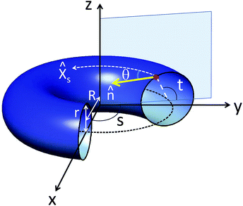 |
| | Fig. 1 Coordinate system used for the surface of a circular torus of axial radius R and revolving-ring radius r. A point on the torus surface is specified by two variables, s and t. In the current work, the properties of the nematic director field , which can be represented by angle θ(s, t), is studied. | |
In this paper, a coordinate system is adopted such that the xy plane coincides with the torus' circular–axis plane and the z axis is the symmetry axis. Any point on the toroidal surface can then be specified by two angular variables, s and t, each varying from 0 to 2π. The variable s specifies a vertical plane that contains the z-axis and makes an angle s with the xz-plane. The variable t specifies a point on the circular ring of radius r, formed from the intersection of this vertical plane with the toroidal surface. We can then specify the coordinates of a point on the torus surface by
| |
x = (R + r cos![[thin space (1/6-em)]](https://www.rsc.org/images/entities/char_2009.gif) t)coss, t)coss,
| (4) |
| | |
y = (R + r cost)sins,
| (5) |
| | |
z = rsins.
| (6) |
The in-plane nematic liquid-crystal ordering on the torus surface is indicated by a nematic director field
(
r), where
r = (
x,
y,
z). This headless unit vector lives on the tangent plane of a point on the torus surface, making an angle π/2 −
θ with respect to the vertical plane that is used to define
s (see
Fig. 1). Hence the director field is entirely described by the function
θ(
s,
t).
3 Defect-free state of the SKTS model: numerical solution
In this section we are only concerned about a nematic director field that contains no nematic dislocations on the entire surface. We assume that the vector field has a rotational symmetry about the z axis. For such a case, we can directly write θ(s, t) = θ (t). While the derivation of the free-energy expression in Appendix A is for both s- and t-dependencies, based on this assumption the SKTS model defined in eqn (2) can be written as a functional of the function θ(t) only,| |
 | (7) |
where| | |
p(t) = k−1 + cost,
| (8) |
and| |
 | (9) |
The constant f0 is| |
 | (10) |
The heart of the problem then becomes minimizing this energy functional.
A number of solutions can be obtained, each corresponding to a branch of the free energy minimum as a function of k. A trivial solution is
We now argue that it is the only solution in the parameter regime
k < 1/2. This can be demonstrated by examining the function
q(
t) defined in
eqn (9), which has a minimum at
t = π,
q(π) = 1 − (
k−1 − 1)
−2; this minimum is positive when
k < 1/2; thus,
q(
t) is definitively positive over the entire
t-range. In view of the fact that both terms within the square brackets in
eqn (7) are quadratic, the only free-energy minimum then corresponds to the trivial solution mentioned above, which produces
F0/2π
K =
f0.
When k > 1/2, this trivial solution remains. Within the regime k ≲ 1 there must be at least two other degenerate free-energy branches beyond the trivial solution. This can be understood by qualitatively analyzing the energy in eqn (7). Along the circle defined by t = π on the toroidal surface, q(π) becomes a large negative number when k → 1; the coefficient of sin2θ is hence negative so that sin2θ prefers its maximum value in order to minimize the local free energy; therefore, within this region on the torus, θ → ±π/2. That is, the nematic director along the t = π line takes a direction that parallels the z-axis. These two preferences are degenerate states that give rise to the same free energy because of the symmetry of the problem. Note that along the outer circle, defined by t = 0, q(0) is always positive; hence locally the nematic director prefers an orientation specified by θ ∼ 0, or in perpendicular to the z-axis. Overall, the competition between these two local preferences introduces a spontaneous symmetry-breaking transition at a critical point kc somewhere between k = 1/2 and 1, destroying the rotational symmetry of the nematic field about the toroidal axis.
It is then clear that a constant-θ can not minimize the total free energy in the symmetry-breaking state. In order to quantitatively find the non-trivial solution θ1(t), we follow the standard procedure to write the Euler–Lagrange equation for optimizing the functional F,
| | |
p(t)q(t)sin2θ + 2sintθ′ − 2p(t)θ′′ = 0.
| (12) |
where
θ′ and
θ′′ denote the first and second derivatives of
θ(
t) with respect to
t, respectively.
The simplest solution, which we label by a subscript 1, follows the symmetry properties of p(t) and q(t) such that
| | |
θ1(t) = θ1(2π + t) = θ1(2π − t).
| (13) |
Though the discussion below is based on a positive
θ1(
t), from
eqn (12) one can see that this solution is always accompanied by another solution −
θ1(
t); the latter specifies a mirror director field, which has a degenerate free energy same as that of
θ1(
t). Numerically solving
eqn (12) we find that such a solution is possible in the region
kc <
k ≤ 1. The discussion in Appendix B leads to the determination of the critical point,
The angle θ1(π) can serve as the order parameter of the symmetry breaking state. In Fig. 2(a), we plot the order parameter as a function of k; near the critical point kc, our numerical solution asymptotically follows the power law
which is expected in a mean-field theory of the second-order phase transition. The bifurcation of the free energy curve at
kc can be observed in
Fig. 2(b), where the free energy of the symmetry-breaking phase has a lower value (solid line) than that of the trivial solution (dashed line). For selected
k in the range [
kc, 1], a few typical examples of
θ1(
t) are plotted in
Fig. 3(a).
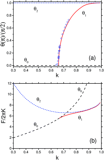 |
| | Fig. 2 Three branches of (a) order parameter θ(π) and (b) reduced free energy as a function of k. The long dashed line represents the trivial solution θ0(t) = 0. The solid curve represents our numerical solution to the Euler–Lagrange equation, eqn (12), discussed in Section 3, for the symmetry breaking phase that has the properties in eqn (13); the diamonds represent our numerical solution based on a simulated Monte Carlo scheme, discussed in Section 4; the dotted line represents the numerical solution for an excited state that follows the symmetry properties in eqn (16). | |
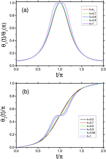 |
| | Fig. 3 Profiles of the nematic director field represented by the function θ(t). For the symmetry-breaking ground state we illustrate θ1(t) in (a) for k = kc, 0.7, 0.8, 0.9 and 1. For the first excited state we illustrate θ2(t) in (b) for k = 0.5, 0.7, 0.8, 0.9, 0.95 and 1. The solution were obtained from numerically solving the Euler–Lagrange equation in eqn (12). Please refer to Fig. 1 for the definition of θ and t. | |
There are, however, other branches of solution to the ordinary differential equation in eqn (12). A particularly interesting one is the first-excited state that follows the symmetry properties
| | |
θ2(t) = −π + θ2(2π + t) = π − θ2(2π −t).
| (16) |
Physically, the director vector changes a value π after it revolves around the torus axis by one circle. While in a high-
k region this metastable state has an free energy (shown in
Fig. 2 by the dotted line) lower than that of the trivial solution, beyond
kc the solution
θ1(
t) corresponds to the ground-state energy hence is most stable. Examples of the numerical solution
θ2(
t) can be found in
Fig. 3(b). Other higher excited states can be obtained for the defect-free nematic field by adding to
θ(
t) a multiple values of π after one complete circular revolution about the torus axis; these are not discussed here.
4 Defect-free state of the Evans model
Now we comment on the Evans model in eqn (1), in which the gradient operator acts on the nematic field covariantly. Physically, because the derivative is taken along a surface direction regardless of the surface curvature, the natural free-energy minimum for a defect-free state is then simplywhere C is an arbitrary constant.
According to Nelson and Peliti, the Evans model can be expressed by the scalar θ(s, t) field,
| | |
FE = ∫[K(∇θ + A)2]dA
| (18) |
where A = (
![[X with combining circumflex]](https://www.rsc.org/images/entities/i_char_0058_0302.gif) s
s·
∂st,
s·∂
tt), and
s together with
t can be found in Appendix A.
21 An elaborative mathematical analysis and discussion of the model is given in
ref. 15. Because
θE can be an arbitrary constant, the defect-free free energy is infinitely degenerate.
For any curved surface, SKTS has shown that
| | |
FSKTS = FE + ∫[K(·K·K·)]dA
| (19) |
where
K is the local curvature tensor on the surface.
17 The main difference between these models is then given by the last term, written in a rather enlightening form. The additional term explicitly couples the nematic order field with the curvature tensor, favoring alignment of the nematic director along a small curvature direction. This is the root for the energetic preference of the non-trivial solution found in the last subsection; in large
k systems, the surface portion near the
z axis,
i.e., at
t = π, has two identifiable main curvature directions: one along
s with a large curvature and the other along
z axis with a small curvature. This term then prefers
θ = ±π on this location, breaking the symmetry of the original trivial solution
θ0 = 0.
5 Defect-free states: simulated annealing Monte Carlo solution
In the above, we have studied the defect-free nematic-director structure on the toroidal surface, represented by θ(t) with the assumption of no s-dependence. To validate this assumption, we conducted simulated-annealing Monte Carlo minimization, including the s dependence in θ(s, t). The detailed numerical procedure, including the representation of the toroidal surface by triangulation, is explained in Appendix D.
Fig. 4(a)–(c) illustrates examples of the nematic director configuration yielded from minimizing the SKTS model. In all three cases, the director field does not depend on s and is a function of t only. Three solutions have been found from our simulations, consistently recovering the θ0, θ1, and θ2 solutions produced in Section 3 from solving the differential equation. While the θ0 solution is typically found in a low k case, the θ1 solution starts to emerge in systems with k > kc. The latter is characterized by the angle that the nematic director makes with respect to the s axis along the t = π line. In Fig. 2(a), we display the Monte Carlo results by diamond symbols, overlapping the red solid curve which represents the solution found from solving the differential equation. The agreement is satisfactory.
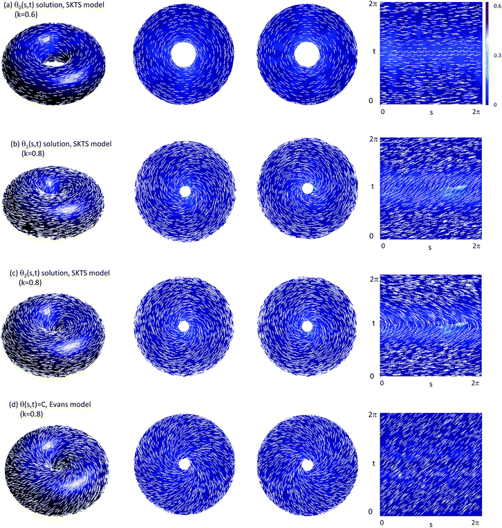 |
| | Fig. 4 Configurations of the defect-free nematic field found from the simulated annealing Monte Carlo procedure. In all cases, the director fields have a rotational symmetry about the z axis, i.e., they do not depend on s. The structures are plotted in three different types of views. The first column of plots corresponds to a three-dimensional view; the second and third columns of plots represent the top (t = [0, π]) and bottom (t = [π, 2π]) views; the fourth column contains an expanded view, where the nematic director field is displayed as a function of s (horizontal axis) and t (vertical axis). The color in all plots represents the local Frank energy, fi, defined in Appendix A, which has a value ranging from low (blue) to high (red). | |
The metastable θ2 solution of the SKTS model, however, always corresponds to a higher free energy than those of the θ0 and θ1 solutions. Normally within a simulated annealing protocol, it is difficult to trap such a metastable state. To obtain the configuration in Fig. 4(c), we enforced the boundary conditions θ2 = 0 at t = 0 and θ2 = π/2 at t = π. These boundary conditions are consistent with the requirement in eqn (16) for the symmetry of the θ2 solution.
Fig. 4(d) illustrates a typical configuration obtained from the simulation of the Evans model. A constant nematic director field is obtained over the entire (s, t) space, which verifies Evans' solution for the covariant energy model.15 The Monte Carlo simulation also features a basic property of this solution: the overall nematic director of this constant field is not fixed. Depending on the initial condition, we obtained configurations that contain different field angles, all within a comparable free-energy range.
It should be noted that the discrete version of the Evans model used in our Monte Carlo study is rather involved mathematically, as discussed in Appendix D. To produce a constant field, various terms in the free energy expression, eqn (37), must be balanced and even cancel each other. The ability of the Monte Carlo procedure to produce a constant field validates both the original Evans solution and the discrete version of the model.
6 States containing nematic-field disclinations
The Monte Carlo procedure allows us to capture metastable free-energy minima by rapidly lowering the simulated temperature. However, a quickly quenching temperature can also trap the simulated system in unwanted high-energy configurations. We have conducted multi-thread Monte Carlo simulations with different annealing schedules of the simulated temperature. In this section we discuss some of the low-energy structures that contain nematic-field disclinations.
These configurations are represented by a θ(s, t) that depends on both variables; the rotational symmetry about the z axis found in the defect-free states is no longer present. Fig. 5(a) illustrates a typical configuration obtained from minimizing the SKTS model, which contains one pair of defects in nematic ordering on the surface of a torus. The result is in compliance with the Poincaré–Hopf theorem22 which indicates that in the current system the winding numbers should sum to zero. The distorted nematic field, shown in the expanded view of Fig. 5(a), contains one disclination at s = π and t ∼ π with a winding number −1/2 and another disclination at s = 0 and t ∼ π/2 with +1/2. This is a structure that was previously found by SKTS.17 The pattern within s = [0, π] is closely related to the defect-free θ2 solution, in which θ0 = 0 at t = 0 turns into θ0 = π at t = 2π; the pattern within s = [π, 2π] is closely related to the defect-free θ1 solution, in which θ1 reaches a maximum at t = π and then returns to its original value at t = 2π. Although the distorted nematic field no longer contains these properties, some reminiscence can be found by comparing Fig. 4(b), (c) and Fig. 5(a).
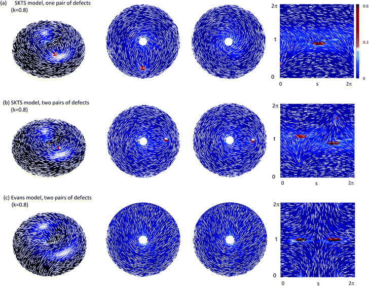 |
| | Fig. 5 Illustration of nematic fields that contain disclinations, obtained from the simulated annealing Monte Carlo procedure. The first column is a three-dimensional view of the structures; the second and third columns are top and bottom views of the structures; the right column is an expanded view of the toroidal surface where the horizontal and vertical axes correspond to s and t respectively. The color in all plots represents the local Frank energy, fi, defined in Appendix A, which has a value ranging from low (blue) to high (red). | |
Fig. 5(b) illustrates a configuration produced from minimizing the SKTS model, where two pairs of ±1/2 defects are visible. Each pair are located in relative positions similar to those found in the one-pair scenario. One ±1/2 pair is separated from another pair by a distance Δs = π; geometrically, in three-dimensions these pairs attempt to separate from each other as far as possible. The director field now follows the symmetry property
| | |
θ(s, t) = θ(π − s, π − t).
| (20) |
A double-pair defect pattern was suggested by SKTS, however, does not display this high symmetry.
A common feature of these defect patterns is that the +1/2 defects are located far away from the z axis where the Gaussian curvature is positive, whereas the −1/2 defects are closer to the z axis, where the Gaussian curvature is negative. Nelson and Peliti made an interesting comparison between electrostatics and surface nemetic field containing disclinations;21 the topological defect on a curved surface behaves in a way similar to a charge in an electrostatic problem. Within this analogy, the positive Gaussian curvature plays the role of a negative charge distribution and a topological defect with a positive winding number plays the role of a positive point-like charge. Hence, the high positive Gaussian curvature region attracts a disclination with a positive winding number. Once this is settled, a defect pair in Fig. 5(b) attempt to rotate about the z axis, separating itself as far as possible from another pair.
Within the SKTS model, the ground state is the defect-free θ0 or θ1 state, depending the magnitude of k. The configurations containing topological defects that we discuss here are metastable excited states. When a pair of disclinations of positive and negative winding numbers approach each other, they might annihilate; however, for a metastable state containing nematic disclinations, there is a free-energy barrier between the two, which prevents them from moving closer to each other. In our simulations, the defect states can be typically stabilized in high k systems. A low-k system, however, cannot create a negative Gaussian curvature region which is essential for sustaining a disclination with a negative winding number. Hence in the Monte Carlo simulations, defect patterns have not been observed on the surface of a thin torus.
For comparison, a typical configuration produced from the Evans model with two pairs of defects, is shown in Fig. 5(c). Similar to the pattern seen in Fig. 5(b), the two +1/2 defects are located in the outer-most region of the torus, and the two −1/2 defects are located in the inner-most region. A interesting feature is that all the defects are located within the middle plane of the torus (t = 0, π). This is the direct result of the mirror symmetry about the middle plane of the orientation field existing in the free energy model. The result produced here is consistent with the theoretically predicted eigenstate 21 by Evans.15 The main difference between Fig. 5(b) and (c), is the symmetry of the fields. In (c), we observe
| | |
θ(s, t) = θ(π − s, t) = θ(s, π − t),
| (21) |
which is quite different from
eqn (20). One defect pair were never stabilized in the Monte Carlo simulation of the Evans model.
7 Summary
In summary, we examined the solution of two commonly used models for the nematic director field on the surface of a torus.15,17 These two models are based on the Frank energy model, but have treated the surface derivatives of the nematic director field differently. The resulting configurations derived from these models, either the defect-free solutions or the solutions containing nematic field disclinations, are quite different.
A definitive answer to which model should be used for comparison with experiments, however, cannot be settled easily. The physical systems described by these two models are different and are reflected by how local nemetic fields interact with each other. For example, in the case of short liquid-crystal molecules confined within a fluid layer of finite thickness, the full three-dimensional derivative presented in the SKTS model is more applicable. On the other hand, in systems where a liquid crystal is completely embedded on the toroidal surface of nearly zero thickness, the Evans model is more applicable; however, in this situation, the rigidity of bent molecules has a preference on the local surface curvature, which most likely has an added effect beyond the covariant energy considered here.
It would be desirable to determine the energy barrier between the metastable states found in Section 6 and the ground states found in Sections 4 & 5 within the current models. The numerical method used here searches for an equilibrium state (energy minimum) of the system; the configuration at the top of the energy barrier gives rise to an energy maximum, which cannot be obtained by the numerical technique presented in this article. In principle, one could map out the energy landscape (hence the energy barrier) between two minima, utilizing for example the Wang–Landau Monte Carlo method, by controlling the relative positions of the two defects (which is a tricky issue). Such a calculation is beyond the scope of the current work where we used the simulated annealing Monte Carlo method.
Appendix
A Derivatives in the energy model
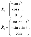
In this Appendix, we express the general form of the gradient derivatives in the energy model in terms of the coordinate system established in Section 2. The parametrization was introduced in Fig. 1.
Together with the introduction of variables s and t, two perpendicular tangent vectors can be introduced on the toroidal surface,
| |
 | (22) |
The covariant form of the metric tensor can then be evaluated from these tangent vectors,
| |
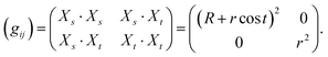 | (23) |
The corresponding contravariant form of the metric tensor is,
| |
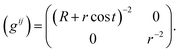 | (24) |
We then have
| |
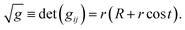 | (25) |
On the basis of these vectors, we write a the nematic director as
where the normalized tangent vectors are
| |
 | (27) |
The expression introduces
θ, an orientation angle of the nematic director on the toroidal surface, as a function of parameters
s and
t,
θ =
θ(
s,
t).
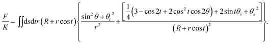
The free energy in eqn (2) can be explicitly parameterized in this representation as
| |
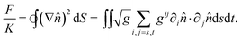 | (28) |
The derivatives of the nematic vectors can be deduced,
| |
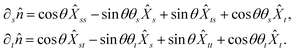 | (29) |
In the above expression, partial derivatives have been written as subscripts. Considering
| |
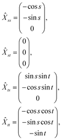 | (30) |
we can finally express the free energy in terms of
θ(
s,
t),
| |
 | (31) |
In Section 3, we specifically deal with systems with a rotational symmetry. The solution corresponds to a θ(s, t) depending on the variable t only. Directly using the notation θ(t) we substitute eqn (24), (25), (29) and (30) into the free energy functional eqn (19). The free energy then becomes
| |
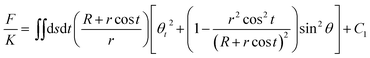 | (32) |
where
C1 is a constant. Now, to find
C1, we can let
θ = 0 and return to the original model to evaluate the free energy, which gives
. This expression is used in
eqn (7) of Section 3.
B Critical k for a non-trivial solution of eqn 12
In the low-k region, eqn (12) has a trivial solution θ0 = 0 only. Beyond a critical kc, a nontrivial solution that follows the symmetry properties in eqn (13), θ1(t), can be obtained.
In order to determine the critical value kc, we construct an eigenvalue problem where λ is the eigenvalue to be determined:
| |
 | (33) |
As a function of
k, the spectrum of
λ is a continuous function with a minimum
λmin. If
λmin > 0, the only solution to the original equation is the trivial
θ0 = 0; if
λmin < 0 a nontrivial solution exists.
23 The requirement
λmin = 0 determines a critical value
k =
kc for the emergence of the non-trivial solution.
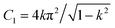
We developed a computational algorithm to evaluate the minimum eigenvalue for different k numerically. The result is displayed in Fig. 6. Examining the intersection with λmin = 0, we obtain kc = 0.659…
 |
| | Fig. 6 The minimum eigenvalue λmin for λ appearing in eqn (33) as a function of k. | |
C Numerical scheme for solving eqn 12
The numerical algorithm used to integrate eqn (12) follows the Runge–Kutta method. A shooting method is employed to incorporate the appropriate boundary conditions into the solution.
For example, to obtain the symmetry-breaking solution that displays the symmetry properties in eqn (13), we need to consider the boundary conditions
| | |
θ′1(0) = θ′1(π) = 0.
| (34) |
Using
θ′1(0) = 0 and a guessed
θ1(0), we integrated the differential equation to obtain
θ1(
t) until
t = π. Then,
θ′1(π) was deduced from the numerical solution. In the next step, we made an attempt to adjust
θ1(0) to match the condition
θ′1(π) = 0. The iteration was terminated after this condition was met.
D Simulated annealing procedure to minimize the free energy
To obtain the free-energy minimum, we developed a general simulated annealing procedure that depends on triangulation of the toroidal surface. For a given k = r/R ratio, the toroidal surface is divided into a triangular lattice of N triangles. The triangle labeled i is associated with an in-plane unit vector i which represents the triangle's local in-plane liquid crystal order.
The unit vector pairs i and j interact with each other only when triangles i and j are adjacent neighbors sharing one common edge. From the center of the ith triangle to this common edge we define an triangle and from the center of the jth triangle to the common edge we define another triangle; the area of these two triangles, Sij, can be calculated. One can then show that within the SKTS model, the free-energy model in eqn (2) is simply expressed by
| |
 | (35) |
where
| |
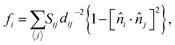 | (36) |
and
dij is the distance between the centers of the triangles
i and
j. The quantity
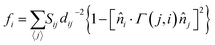
fi is the local energy cost.
The discrete notion for the Evans free energy, eqn (1), however is more involved. We can show
| |
 | (37) |
where
| |
 | (38) |
is the local energy cost. The operator
Γ(
j,
i)
j transports the vector
j from triangle
j to
i and then projects it on triangle-
i's surface; the expression can be found in
ref. 24.
These two free energies were used in a simulated Monte Carlo procedure for minimization purpose. To start, we generated an initial configuration that contained randomly assigned directions on the nematic directors of all lattice triangles. At each Monte Carlo trial, the nematic vector of a random selected triangle was randomly rotated within the tangent plane. The Metropolis rule that entails the transition probability
| | |
T = min{1, exp(−βΔF/K)}
| (39) |
was then incorporated for deciding whether the trial move is accepted, where Δ
F is the free energy difference between the free energies after and before the move. Within a simulated annealing protocol, to produce the defect-free states the simulated temperature 1/
β was set at a high value and then lowered in every 5000 Monte Carlo steps by a factor of 1/1.0005. When 1/
β was sufficiently low so that a definite configuration emerged, the computation was stopped. All results discussed in this paper were obtained from a triangulation scheme that contained
N = 4 × 10
4 surface triangles.
Acknowledgements
We thank the National Nature Science Foundation of China (funding numbers 10874111, 11304169 and 11174196), the 111 project of the Education Ministry of China (funding number B14009), and the Natural Science and Engineering Research Council of Canada for financial support. We also thank Prof. X. Xing for helpful discussion on the research topic. Note added in proof: Segatti, Snarski, and Veneroni have independently studied some issues related to the same problem discussed in this paper. Please see arXiv:1401.6038 [math-ph] or Phys. Rev. E (in press).
References
- D. R. Nelson, Defects and geometry in condensed matter physics, Cambridge University Press, 2002 Search PubMed.
- M. J. Bowick and L. Giomi, Adv. Phys., 2009, 58, 449–563 CrossRef CAS.
- T. C. Lubensky and J. Prost, J. Phys. II, 1992, 2, 371–382 CrossRef CAS.
- D. R. Nelson, Nano Lett., 2002, 2, 1125–1129 CrossRef CAS.
- H.-L. Liang, S. Schymura, P. Rudquist and J. Lagerwall, Phys. Rev. Lett., 2011, 106, 247801 CrossRef.
- T. Lopez-Leon, V. Koning, K. B. S. Devaiah, V. Vitelli and A. Fernandez-Nieves, Nat. Phys., 2011, 7, 391–394 CrossRef CAS.
- H. Shin, M. Bowick and X. Xing, Phys. Rev. Lett., 2008, 101, 037802 CrossRef.
- M. A. Bates, J. Chem. Phys., 2008, 128, 104707 CrossRef PubMed.
- W.-Y. Zhang, Y. Jiang and J. Z. Y. Chen, Phys. Rev. Lett., 2012, 108, 057801 CrossRef.
- W.-Y. Zhang, Y. Jiang and J. Z. Y. Chen, Phys. Rev. E: Stat., Nonlinear, Soft Matter Phys., 2012, 85, 061710 CrossRef.
- Y. Li, H. Miao, H. Ma and J. Z. Y. Chen, Soft Matter, 2013, 9, 11461 RSC.
- G. A. Devries, M. Brunnbauer, Y. Hu, A. M. Jackson, B. Long, B. T. Neltner, O. Uzun, B. H. Wunsch and F. Stellacci, Science, 2007, 315, 358 CrossRef CAS PubMed.
- Z.-C. Ou-Yang, Phys. Rev. A, 1990, 41, 4517–4520 CrossRef CAS.
- M. Mutz and D. Bensimon, Phys. Rev. A, 1991, 43, 4525–4527 CrossRef CAS.
- R. M. Evans, J. Phys. II, 1995, 5, 507–530 CrossRef CAS.
- M. Bowick, D. R. Nelson and A. Travesset, Phys. Rev. E: Stat., Nonlinear, Soft Matter Phys., 2004, 69, 41102 CrossRef.
- R. L. B. Selinger, A. Konya, A. Travesset and J. V. Selinger, J. Phys. Chem. B, 2011, 115, 13989–13993 CrossRef CAS PubMed.
- B. Senyuk, Q. Liu, S. He, R. D. Kamien, R. B. Kusner, T. C. Lubensky and I. I. Smalyukh, Nature, 2013, 493, 200 CrossRef CAS PubMed.
- M. Cavallaro Jr, M. A. Gharbi, D. A. Beller, S. Čopar, Z. Shi, R. D. Kamien, S. Yang, T. Baumgart and K. J. Stebe, Soft Matter, 2013, 9, 9099 RSC.
- T.-S. Nguyen, J. Geng, R. L. B. Selinger and J. V. Selinger, Soft Matter, 2013, 9, 8314 RSC.
- D. R. Nelson and L. Peliti, J. Phys., 1987, 48, 1085–1092 CAS.
- M. P. Do Carmo, Differential geometry of curves and surfaces, Prentice-Hall, Englewood Cliffs, NJ, 1976 Search PubMed.
- J. D. Pryce, Numerical solution of Sturm-Liouville problems, Clarendon Press, Oxford, 1993 Search PubMed.
- N. Ramakrishnan, P. B. S. Kumar and J. H. Ipsen, Phys. Rev. E: Stat., Nonlinear, Soft Matter Phys., 2010, 81, 041922 CrossRef CAS.
|
| This journal is © The Royal Society of Chemistry 2014 |
Click here to see how this site uses Cookies. View our privacy policy here. 


 . This expression is used in eqn (7) of Section 3.


