Heterogeneous catalyst discovery using 21st century tools: a tutorial

Abstract

In this tutorial we highlight the optimal working methodology for discovering novel heterogeneous catalysts using modern tools. First, we give a structure to the discovery and optimisation process, explaining its iterative nature. Then, we focus in turn on each step of catalyst synthesis, catalysts testing, integrating low-level and high-level descriptor models into the workflow, and explorative data analysis. Finally, we explain the importance of experimental and model validation, and show how by combining experimental design, descriptor modelling, and experimental validation you can increase the chances of discovering and optimising good catalysts. The basic principles are illustrated with four concrete examples: oxidative methane coupling; catalytic hydrogenation of 5-ethoxymethylfurfural; optimising bimetallic catalysts in a continuous reactor system, and linking material properties to chemisorption energies for a variety of catalysts. Based on the above examples and principles, we then return to the general case, and discuss the application of data-driven workflows in catalyst discovery and optimisation.

---

1. Introduction

Research in the discovery of novel heterogeneous catalysts faces an enormous challenge in years to come. With the now commonly acknowledged abundance of fossil resources like shale gas, refineries around the world will shift feedstocks from oil to gas. This requires novel catalytic pathways to, for example, C₂–C₄ olefins^1–4 and aromatics.^5–7 Where many of these molecules are now extracted from oil or its subsequent cracking product in the refining process, novel processes are needed considering light alkanes like methane, ethane and propane as the feeds.^8,9 Concurrently, the field of biomass conversion is maturing. Several processes producing building blocks based on biomass will come online in the next two decades. In this area, catalytic processes are required for converting these building blocks to products. These products include both drop-ins like ethylene from ethanol,¹⁰ butanediol from succinic acid¹¹ and aromatics from alcohols,¹² as well as new-to-world products like furan dicarboxylic acid (FDCA),^13,14 a novel monomer for polyesters, and farnesene,^15,16 a novel fuel and lubricant component. Regardless the nature of the final product – catalysis will be needed to perform the final steps of the process.

Since catalysis research is a multifaceted problem, involving variations in catalyst composition and experimental conditions, a systematic research methodology is required. Doing only experiments is not enough. The experiments are better combined with modelling at various degrees of complexity is required to effectively discover catalysts for new or existing processes.

Applying modelling methods will benefit all stages of catalyst development, provided that the appropriate level of complexity is applied at each stage. As a general rule, model complexity should increase as a project progresses. Initial stages need relatively simple methods from chemometrics (exploratory data analysis) and experimental design (empirical modelling). Later stages will benefit from more rigorous, kinetic models. Note that the “users” of models and data differ at the various stages. In early stages, the target audience is mostly composed of research chemists. Later, the focus shifts to providing chemical engineers with sufficient information to design pilot-scale processes. Indeed, involving the engineers from the start is the key to success.^17,18

This tutorial focuses on empirical modelling methods, illustrating them with three case studies: first, we discuss statistical experimental design on the oxidative coupling of methane. This chemistry is receiving an increased amount of attention in both academia and industry^19,20 with the expected price developments for methane resulting from shale gas production. Then, we review the use of exploratory data analysis with principal component analysis (PCA) and descriptor–performance relationships using hydrogenation of 5-ethoxymethylfurfural (EMF).^21–23 Finally, we explain the development of generic descriptors for metals using a computationally-derived database of heats of adsorption of gases on metals.²⁴ The latter approach is then validated against the experimentally measured adsorption of gases on titania-supported metals.

Note that while a part of this tutorial focuses on using large data sets generated by parallel reactor technology, our primary objective is not explaining high-throughput experimentation. Instead, we focus on data analysis and modelling methods that help to maximize learning from these large data sets. Specific information on the various uses, strengths and weaknesses of parallel reactors are available elsewhere.^18,25,26

2. Typical workflow for catalyst development

To understand better the use of empirical modelling methods, let us first examine the unit operations of the typical workflow for catalyst development (Fig. 1). The guiding principle of this workflow is that it is an iterative process, not a linear one. After each set of experiments, the results are compared against the objectives. If these are met, you may proceed to next stage. Otherwise, if the data indicates that your initial objectives are unrealistic, these objectives must be adjusted.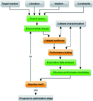

Fig. 1 Flow diagram representing a typical workflow for the development of (heterogeneous) catalysts.

The empirical modelling methods (highlighted in green in Fig. 1) are the focus of this tutorial. We also discuss briefly some other elements of the workflow, namely catalyst synthesis and testing.

2.1. General comments regarding precursor selection and catalyst synthesis

The key to a successful scale-up of catalyst synthesis is using simple methods. Straightforward steps like impregnation and precipitation can be scaled up relatively quickly to produce kilograms of catalyst. Even for the simplest impregnation (Fig. 2) many steps and variables have to be considered. Since several excellent books have been published on this subject,^27,28 we only highlight a few key points here.

Fig. 2 Typical steps in catalyst synthesis via impregnation. Note that some steps, in particular the dissolution and impregnation steps, may need to be carried out multiple times.

First, we consider the starting materials. Commercially accessible materials are preferable. This holds for both the carrier, in the case of a supported catalyst, and for the metal precursors. We also keep in mind the conditions that the catalyst will be exposed to during its synthesis and testing. The support must maintain its structural integrity during calcination and reduction. Well known examples include the anatase–rutile transformation observed for titania²⁹ and ceria structural collapse³⁰ at high temperature. The precursor salt should be readily transformed to an oxide or metal during calcination and/or reduction. As a rule of thumb, metal nitrates are preferable over chlorides. Most nitrates require calcination temperatures between 250 and 400 °C, while chlorides typically require temperatures between 500 and 700 °C. If a metal is prone to sintering or agglomeration, its chloride precursor is more likely to give a lower active metal surface area. Likewise, organic anions such as acetate or oxalate introduce the risk of carbon deposits on the catalysts. Examples of catalysts that can be synthesized using straightforward methods in the laboratory are Pd/Al₂O₃ for hydrogenation³¹ and AuPd/SiO₂ for vinyl acetate synthesis from acetic acid and ethylene.³²

The accuracy of small-scale preparations (milligrams to grams of catalyst) benefits from minimizing the number of steps (i.e. running a more dilute, single-step impregnation). In the case of bimetallic (or multimetallic) catalysts you must choose between single-step (co-impregnation) and sequential impregnation. We advise trying out both methods on a small number of catalysts before preparing large libraries. Co-impregnation is simpler, but sequential impregnation is preferable when the difference in solubility for two precursor salts is large. One such example is the synthesis of the supported Pt–Sn catalyst used in the reduction of α,β-unsaturated aldehydes and the dehydrogenation of alkenes to olefins or aromatics. Here the solubility of platinum nitrate is high, while the solubility of tin acetate is low. Unless you need very low tin loadings, this impregnation requires two (or more) steps.³³

When considering parallel reactors for catalyst testing, certain compromises will have to be made in catalyst synthesis. Consistency here is of the utmost importance to avoid confusing catalyst components and catalyst synthesis being responsible for activity. Ideally, in each set of experiments, the synthesis of catalysts is kept as constant as possible. This applies to the precursors used, the synthesis method, and the post-synthesis steps (drying, calcinations, reduction). Not all catalysts will be prepared using optimized conditions. To minimize the risk of “missing out” on potentially promising leads, it is good practice to at various stages in a research program include subsets of experiments where these parameters are addressed or revisited. Especially in early stages of a study, an experimental campaign that probes the impact of synthesis variables on the performance of a limited set of catalysts is valuable. First, the information can be translated in a synthesis protocol for use during screening. Second, the potential gains that can be obtained by optimizing the synthesis of an identified lead can be quantified.

2.2. General comments regarding catalyst testing

When testing a catalyst library, defining a uniform test protocol is important. Here the key parameters are the activation procedure, the catalysts' stability, the reference conditions, and the analysis methods. In the following paragraphs we briefly address these topics. A more detailed discussion of common synthesis methods and testing protocols is given in the books edited by Ertl²⁷ and Regalbuto.²⁸

First, let us consider the catalyst activation procedure. Often, a simple reduction step followed by a short equilibration with the feedstock will suffice. One notable exception is hydrodesulphurization, which requires a sulfiding step using a sulphur donor (typically H₂S, polysulfides or Me₂S₂). Another is the Fischer–Tropsch synthesis, where the catalyst must be equilibrated under reaction conditions for up to two weeks before reaching steady-state performance.³⁴ While the optimal activation method may differ between individual catalysts, using a consistent testing method makes comparing the performance data easier.³⁵

The second factor we must consider is catalyst stability. If catalysts are known to have a limited lifetime, the number of experimental conditions that can be explored needs to be limited. In case lifetime is not a concern, longer run times can be used and thus more data points per catalyst can be obtained. In a flow reactor the experimental conditions that can easily be varied on stream are (a) temperature (b) space velocity (c) pressure and (d) feed composition. If the experimental conditions are varied during testing, you must frequently return to a reference condition with known performance. As long as this performance does not change, you can assume the catalyst has not changed.¹⁸

In most cases, the compositional analysis of products is the bottleneck of catalyst testing. This is true even for simple gas-phase reactions. The common techniques are chromatography and spectroscopy. The key advantage of chromatography is that the components in the reactor effluent are separated and thus easily quantified. The disadvantage is the time-consuming analysis. Assuming the composition of reactor effluent can be determined in five minutes using GC, one still needs over five hours to analyse 64 reactors.³⁶ Conversely, spectroscopic analysis enjoys the advantage of speed, but suffers from the fact that all components are analyzed simultaneously. This means the concentrations of individual components must be extracted by means of multivariate calibration and/or deconvolution.^37,38

3. Integrating modelling methods in catalyst research

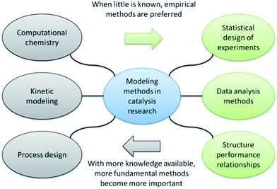
For clarification, we will divide the modelling methods in catalysis in two groups: fundamental and empirical (Fig. 3). The first group, which includes computational chemistry, kinetic modeling and reactor design, focuses on reaction mechanisms and engineering principles. Such methods are useful when mechanistic information and/or reactor constraints are available a priori. The second group includes data-driven models that make no assumptions on reaction mechanism or the reactor configuration. They can therefore be applied early in the research when little information is available.

Fig. 3 Modeling methods used in catalysis research. The empirical methods are highlighted in green on the right hand side of the diagram. The more fundamental methods are located on the left hand side of the diagram.

In contrast to popular belief, modelling methods in catalysis are best used in an integrated manner. Synergy is achieved only by close collaboration between the modelling and experimental teams. The largest hurdle here is the “language barrier” between researchers from different disciplines. Strikingly, the empirical (data-driven) methods pose the most difficulties. This is because they are typically practiced by statisticians rather than chemists or chemical engineers. In this tutorial, we will highlight the useful information obtainable by combining empirical models with experiments.

Statistical experimental design and principal component analysis are known methods, and using them during research will not lead to the discovery of new catalysts as such. It will, however, lead to a more detailed understanding of the impact of process parameters on catalytic performance. Moreover, you will get a deeper understanding of the relationships between the various performance indicators. Thus, using these existing methods as an integrated part of catalyst development will enhance the chances of identifying new avenues.

3.1. Statistical experimental design

Using appropriate experimental design methods will increase the chances of success for a project in all its stages, from very early screening to the final optimization of catalyst composition and process conditions. The key here is selecting the proper variables. The more complex your system, the more experiments you'll need for exploring the parameter space. But experimental design does more than just minimize the number of experiments. It also ensures that you run the correct type of experiments.

A typical experimental design campaign has three main stages: (1) factor screening, (2) optimization and (3) robustness testing. During factor screening, a large number of variables is explored using a small number of experiments. The objective here is eliminating variables that have only a small effect on the performance. Only the variables that have relevance progress to stage (2), the optimization stage. This stage then provides a quantitative relationship between the variables and the responses. The robustness stage (3) is a sensitivity analysis, providing an assessment of the expected stability of the optimized system.

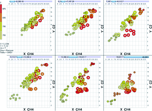
A good experimental design also allows the data to be analyzed as a model instead of as a mere collection of points. As an example, let us consider of the behaviour of a Mn-promoted Na₂WO₄/SiO₂ catalyst in the oxidative coupling of methane. We tested this catalyst in a 64-channel parallel fixed bed reactor at various experimental conditions. The temperature was varied over the range 755–875 °C, the pressure over the range 0–2.5 barg, the GHSV over the range 6000–36 000 h⁻¹ and the methane to oxygen stoichiometry over the range 4–8 molar equivalents. With so many variations, the raw data for even a single catalyst is overwhelmingly complex (Fig. 4).

Fig. 4 Raw performance data for the oxidative coupling of methane over a Mn-promoted Na₂WO₄/SiO₂ catalyst. The vertical axis denotes the combined yield of ethylene and ethane. The horizontal axis denotes the conversion of methane. Marker color denotes the reaction temperature and marker size denotes the reaction pressure. The plot is split in panels based on the space velocity used during the experiment.

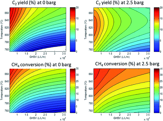
However, since the conditions were varied systematically, we can calculate a response surface model. Here, the parameters (temperature, pressure, GHSV and stoichiometry) are related to the responses (conversion, yields, selectivities). The resulting models can be used to identify the optimal conditions that will give optimal performance. As an example, Fig. 5 shows a set of response surfaces based on the data shown in Fig. 4. We see that the highest methane conversions are found at the lowest space velocities combined with the highest temperature. Less obvious from the raw data, but very clear from the response surfaces: the temperature required to achieve maximum C2 yield shifts from 875 °C at 0 barg to 825 °C at 2.5 barg. Another important observation is that the absolute maximum C2 yield is 16% at 2.5 barg, whereas at 0 barg a maximum yield of 19% can be obtained. For clarity, we show here only two of the key responses, but the other two (CO₂ selectivity and ethylene–ethane ratio) can also be described by similar models.

Fig. 5 Response surfaces for the CH₄ conversion (bottom row) and C₂ yield (top row) at 0 barg (left column) and 2.5 barg (right column) as a function of temperature (vertical axis) and GHSV (horizontal axis). The value of the responses is mapped using the color scale on the right hand side of each panel. The methane : oxygen ratio is 4 : 1. The white area in the plots at 0 barg indicate predicted conversion and selectivity <0%.

Note that response surface models typically use continuous parameters and responses. When categorical parameters are used (for example “good” or “bad” performance or “support 1” and “support 2”), separate response surfaces have to be constructed for each setting.^39,40 Alternatively, one can use classification models.

3.2. Explorative data analysis

Data overload is a big problem with parallel experiments. The best solution is using a database for storage and combination of data. Database platforms (for example SQL, Oracle, MySQL or even Microsoft Access) have many benefits over simple spreadsheets. The most important of these is the ease of linking and combining information from various sources into a single table. Information on the materials used, catalyst synthesis, experimental conditions, raw analytical data and calibration data must all be combined into a single table that tells you what the performance of each of the catalysts is at each experimental condition.

Once the data set is constructed the initial visual exploration of the data can start. Here the total data set needs to be considered. Particular attention is needed for the identifying outliers. These must be studied, and where appropriate removed prior to any model-based data analysis. In this stage it is also important to check the stability of process parameters like temperature and pressure. Several commercial software packages are available to facilitate the visual interpretation of data (for example Spotfire, Miner3D and Tableau). However, keep in mind that interpreting plots mapping many dimensions is difficult (Fig. 4, for example, was generated using Miner3D and is a typical multi-dimensional representation of data).

When the initial exploration of the data set is complete, model-based evaluation can start. One of the most common methods here is principal component analysis (PCA). PCA aims to reduce the number of dimensions of a data set whilst preserving as much as possible the variability. Using PCA, you can extract the key factors. These are the principal components, or PCs (sometimes also called the latent variables). Each PC is a linear combination of the original variables, but unlike the original variables, which may be correlated with each other, the PCs are orthogonal (i.e., uncorrelated, independent of one another, see Fig. 6).

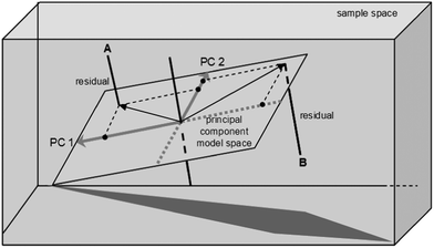Fig. 6 PCA reduces the dimensionality of the problem by projecting the original dataset onto a lower-dimension PC model, in which the new variables are orthogonal to each other. The distance from point A to the PCA model space equals the residual value for catalyst A (reproduced with permission from ref. 22).

To demonstrate the usefulness of PCA, we show the data and PCA analysis thereof for the selective hydrogenation of 5-ethoxymethylfurfural (EMF).^22,23 As with all α,β-unsaturated aldehydes, the primary reaction products are an unsaturated alcohol and a saturated aldehyde. Both primary products undergo various sequential hydrogenation and hydrogenolysis reactions, resulting in a rather complex reaction network (see Fig. 7) with eight products occurring in significant amounts (>5% molar yield). In this case only two principal components are needed to explain 70% of the variation in the data. That means that interpreting the data for a large part can be done by looking at a single two-dimensional plot of the PCs, which is an easier task than identifying trends in the original eight conversion-selectivity plots.

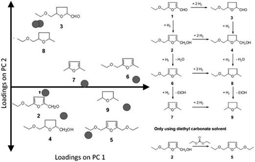Fig. 7 Loadings for the individual yields of products 2–8 occurring in the selective hydrogenation of EMF (left) and the reaction network for the reaction (right).

PCA gives us in two pieces of information: first, the loadings (P) tell us how the individual yields contribute to the structure of the data set. From the loadings plot we can learn a number of things (Fig. 7). First, we see that the loadings for all yields are positive in the first principal component (the horizontal axis in Fig. 7) – this indicates that all yields go up in this direction. In other words PC1 primarily gives information about activity. When considering PC2 the loadings for the yields of 3 and 8 are almost at the same coordinate. This indicates that, no matter what changes are made to catalyst or conditions, the yields of these two components will always increase or decrease together. This is important, because if the objective is maximizing the yield of one of these products alone, the PCA model tells us this is impossible.

Second, the scores on the principal components (T) tell us how each observation relates to the total data set. Since here we base our PCA model on the yields, if two data points are close together in scores space they will have a similar product distribution. In contrast, if they are far apart they will have a rather different product composition. This is easily demonstrated using the scores plot (Fig. 8). Here we see two distinct clusters. The cluster in the upper right quadrant corresponds to a set of Pd/Al₂O₃ catalysts with various promoters tested at temperatures of 100 and 120 °C. At these temperatures this group catalysts favours ring hydrogenation. The cluster in the bottom right quadrant is composed of a set of Rh/Al₂O₃ and Pt/Al₂O₃ catalysts tested at 120 °C. The common factor here is the preference of these catalysts to carbonyl reduction products, leaving the furan ring intact. Both clusters are on the right hand side of the plot, indicating (near) complete conversion.

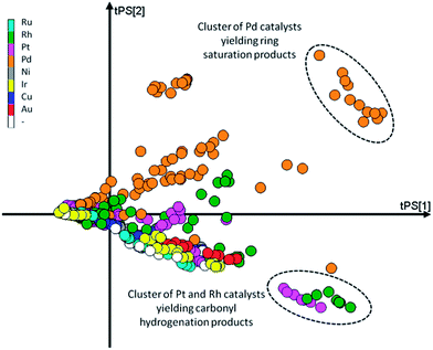Fig. 8 Scores plot for the PCA model with the markers coloured as a function of the main metal used for the catalyst.

3.3. Descriptor–performance relationships for heterogeneous catalysis

The development of descriptor performance relationships for heterogeneous catalysts is hampered by the fact that the active site of a heterogeneous complex is often poorly defined. In contrast, in homogeneous catalysis the entire catalyst is a well defined, molecular complex that can readily be described by common computational chemistry software. This is reflected in the number of publications describing successful applications. For homogeneous catalysis, the last 20 years yielded many published examples.^41–44 For heterogeneous catalysis examples are scarce.^45,46 A number of publications based on the use of density functional theory (DFT) are available.^47–49 Although valuable to gain fundamental insights, using these methods in virtual screening for new catalysts is limited due to the cost of these computations.⁵⁰ In fact, in the time required to model even a small number of catalysts using DFT, many catalysts can be synthesized and tested in real life. Alternatively, using simple, readily accessible descriptors for the metals on the catalyst surface can help us create descriptor–performance relationships.

3.3.1. An example – the selective hydrogenation of EMF. One of the most important differences between heterogeneous and homogeneous catalysis in descriptor modelling is the maturity of the available tools. In homogeneous catalysis, the last two decades of research have resulted in many theoretical descriptors. These range in complexity from simple atom and group counts to topological maps derived from graph theory to geometrical descriptors of varying complexity. Open source and commercial software packages are readily available. In heterogeneous catalysis this is different. Here available descriptors are often difficult to obtain and are typically derived from DFT studies or extensive characterization of the catalysts. These methods, albeit of tremendous value for fundamental insights, are time consuming and require specialist knowledge. Catalyst characterization as a means to derive descriptors related to performance poses another issue: one first needs to synthesize a catalyst, making “virtual screening” a challenging task.⁵⁰

Underlying these challenges in heterogeneous catalysis is the nature of the catalyst. In homogeneous catalysis, catalysts are typically well-defined molecular complexes. Heterogeneous catalysis is much more complex, as the support and metals each play multiple roles.

One practical approach, which we presented for assigning descriptors for modelling heterogeneous catalysts, is using simple bulk properties of the metals. We showed recently that even a complex reaction like the hydrogenation of EMF (reaction scheme in Fig. 7) can be described by correlation of bulk properties of the metals used with the yields of the main components.²¹ To simplify the problem, we kept the support material and catalyst synthesis method used constant. This allows us to focus our efforts in terms of descriptors on the metals used alone. The descriptors we used were derived from Slater-type orbitals for the metals. Instead of using the entire orbital function, we describe the curve be a number of peak parameters often encountered in chromatography and spectroscopy. These simple parameters, the magnitude and location of the peak apex, the width at half height and the skewness, are surprisingly well capable of correlating the metal used with the yields of the main products of the reaction. To establish the validity of the method we first explored a small data set for monometallic catalysts (Fig. 9). After establishing that this model performs well, we extended the data set to bimetallic catalysts, again obtaining good model performance (Fig. 10).

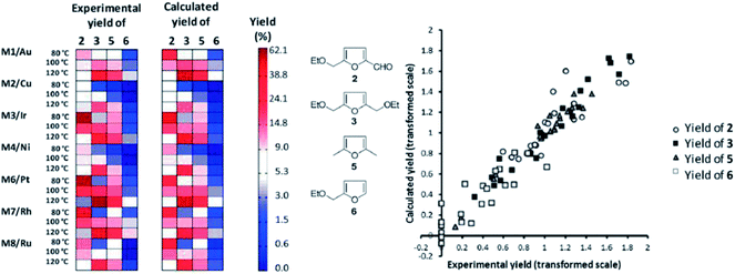Fig. 9 Matrix plot comparing observed yields (left) to the yields predicted by the OPLS model (right). The products are grouped in columns, the catalysts and temperatures are grouped in rows. The yields are coded from light (low yield) to dark (high yield). Both predicted and observed yields are plotted on the same scale. On the right hand side a parity plot representing the same information is given to facilitate interpretation [adapted from ref. 21, with permission].

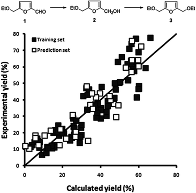Fig. 10 Observed vs. predicted plot for 48 bimetallic catalysts tested at 3 temperatures for the combined yield of 2 and 3. The horizontal axis shows the predicted yields by our model, the vertical axis shows the experimentally obtained yield. The quality of the model is as follows: training set R² = 0.83; RMSEE = 3.7 and prediction set Q² = 0.79; RMSEP = 9.1. [reproduced from ref. 21, with permission].

One important characteristic of empirical modelling methods needs to be emphasized here. Since there is no underlying theoretical model describing the reaction, an empirical model will happily predict negative yields or conversions exceeding 100%. This means that such a model should always be validated chemically and statistically. Luckily, most statistical modelling methods provide this information as an integrated part of the method. When using these methods to design a next set of catalysts for further testing a special situation occurs. For any empirical model a simple rule of thumb is that predictions can be made only over the range of data that was used to create the model. In other words, if a model is regressed using data over a yield range of 0 to 70%, that model will not be able to reliably predict yields great than 70%. Thus, if the objective for a next set of catalysts is increasing the yield beyond 70%, you need to extrapolate. In practice, each next set of catalysts will be based on predicted performance just outside the current range of data. By refitting the model after each set of experiments the valid yield range for the model is extended in an iterative manner.

3.3.2. Developing new descriptors. In contrast to the field of homogenous catalysis, the scientific literature documenting descriptors for heterogeneous catalysts is sparse. Several groups published successful examples of the application of DFT simulations to describe reaction networks. Application of the d-band center as a descriptor is also referred to in many occasions. When turning our attention to simple, empirical descriptors the number of references is even lower. On the basis of this less than abundant literature it is safe to assume that there is a need for documented cases of descriptor development. For these cases it would be important that not only their application is documented, but also sufficient information is provided to allow a researcher to use and extent the method in their own work. As an example, we present here the development of descriptors related to adsorption of gases on metal surfaces.²⁴ Here we developed an empirical model to describe a large database of DFT computations, coupling the heats of chemisorption of 10 different gases to simple, tabulated properties of these gases and the 13 different metals. Using this correlation (Fig. 11) between descriptors and computationally derived chemisorption data, we then extended the method to experimental data of real catalysts. The models are sufficiently robust for application as a more general set of descriptors (Fig.12).

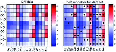Fig. 11 Comparison of the heats of chemisorption obtained using DFT (left) and a simple empirical model based on descriptors (right). The cells with dots indicate the metal–adsorptive combinations that have been used to construct the empirical model. [Adapted from ref. 24 with permission].

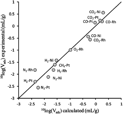Fig. 12 Comparison of isobaric adsorption volumes for supported metal catalysts obtained using experiment (vertical) and simulation (horizontal). The support in all cases was TiO₂, the adsorptive–metal combinations are indicated in the plot. [Adapted from ref. 24 with permission].

This empirical correlation that links easily obtained properties to a phenomenon that is crucial to heterogeneous catalysis, is valuable. Without extensive computations, one can quickly test a few ideas and get a feel for their viability, thus saving the experiments for those ideas that have most merit. As with any empirical model, one has to consider its range of applicability. Luckily, the modelling methods used to establish these models provide an assessment of how valid a prediction is. Moreover, if a prediction is invalid, the same statistics can be used to design a set of experiments (or computations) that allow extension of the model in the desired direction.

Note that the example shown is, indeed, just an example. Many different types of descriptors are typically needed to describe a problem. This is true especially when the catalyst attributes associated with good performance are not well known upfront and have to be established experimentally. When developing descriptors two guiding principles should be considered: (1) a set of descriptors should be accessible for most (preferably all) metals used in catalysis and (2) it should be sufficiently powerful in explaining catalyst performance on its own. The first guideline is easily explained. Imagine using three blocks of descriptors, each having a limited set of metals to which they can be applied. The search space that can be addressed using these descriptors is limited to those metals that can be captured by all three descriptor blocks. The second guideline is more complex. Since typically many different attributes need to be taken into account to explain catalyst performance, the correlation with activity or selectivity of a single attribute is often weak. In those cases, one needs to focus on significance of a correlation (or covariance) rather than its magnitude. Luckily, in the field of homogeneous catalysis these procedures are tried and tested.

3.4. Using descriptor models in catalyst discovery

Now that we have a toolbox that provides the means of designing experiments, modelling the outcome thereof and even generating novel descriptors to meet our needs, we need to consider how to apply these methods effectively and efficiently. We will demonstrate this on the selection of a subset of bimetallic catalysts from a large set of candidates.

First, we designate a set of metals as “Main metal” (highlighted in blue in Fig. 13). Second, we designate a set of metals as “Dopant” (pink, in Fig. 13). These metals, or rather their bimetallic combinations, we characterize with the descriptors based on Slater-type orbitals (see example on selective hydrogenation and ref. 21). Please note that as many (or as few) descriptors can be used as are required by the problem at hand. If you know little about a problem, it is generally better to select more descriptors to start with. After performing a first round of experiments the redundant descriptors can be excluded based on data rather than on assumptions. Finally, we select a number of supports (SiO₂, Al₂O₃, TiO₂, ZrO₂, Nb₂O₅, MgO and ZnO). For each of these supports we select a high and a low surface area. Due to the natural difference in practically accessible surface areas between different supports, the surface area is treated in a relative rather than an absolute manner. Besides surface area, the supports are characterized using their point of zero charge.

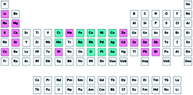Fig. 13 Selected candidate space for our selection problem. Entries in blue are selected as main metals and entries in purple are selected as dopants.

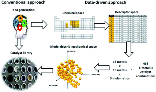
Dopants were applied in molar ratios of 0.05, 0.1 and 0.2 relative to the main metal. The first set of candidates consisted of all the combinations of one main metal and dopant at 3 levels, 13 × 16 × 3 = 624 combinations. The second set was composed by combining two main metals at three dopant levels, giving 13 × 12 × 3 = 468. The total candidate set contained therefore 624 + 468 = 1092 bimetallic combinations. Note that this assumes the use of a single support and a single loading of the main metal. If support variations are included, one could conceive using seven common supports, each with classified by its isoelectric point. Were we to include surface area of this support, for example in a “high” and “low” fashion, the number of supports available in the candidate set would increase to 14. This increases the size of our candidate set to 14 × 1092 = 15 288. Here we assume that surface area, if important at all, will correlate with performance in a linear fashion (since we only use two levels, low and high, we only have enough degrees of freedom to explain the two coefficients corresponding to a straight line). For metal loading, we will not make this assumption. Instead, we will assume that the effect of metal loading is non-linear and we will use 3 levels. This increases the size of the candidate set to 3 × 15 288 = 45 864 catalysts!

Since we cannot synthesize and test over 45 000 catalysts, we must take a stepwise approach. Assuming we can describe the properties of the bimetallic combination by approximately 10 descriptors, we have ten metal parameters + two support parameters + one loading parameter = 13 variables that play a role. As we do not know a priori whether the relationship between variables and performance is linear, we will assume it is nonlinear. Assuming a second order model, we need to identify an intercept, 13 main effects, 12 × 11 = 132 two-variable interactions and 13 quadratic terms. This total of 157 model coefficients is the minimum number of degrees of freedom we need to consider. Adding some replicates (or near neighbours) and some points to determine lack of fit raises this to a number around 200 catalysts that would need to be synthesized and tested. This is a number that is well within reach for most chemistries using state of the art parallel reactor technology. Note that this initial design only comprises 0.4% of the original search space.

To efficiently select candidates from this search space, we first reduce its dimensionality using PCA (see also the example on selective hydrogenation). In this case, over 98% of the variance in the set of candidates is captured by six principal components. Using experimental design (minimal point designs and distance based designs) we can select an optimal subset of catalysts for a first round of experiments. Note that machine-based selection methods are preferred over human intuition, to avoid any bias. Still, intuition not be ignored, so adding more candidates based on “gut feeling” is certainly recommended.

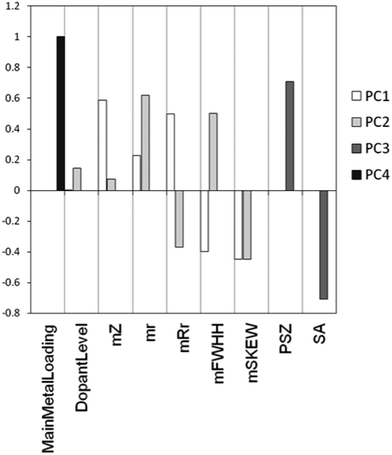
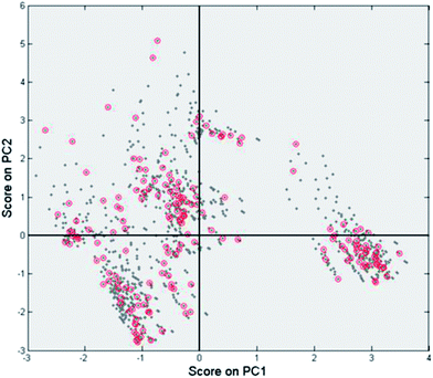
As we explained above, a PCA model is characterized by two matrices: the scores and the loadings. The loadings matrix gives information about the contribution of each of the original variables to each of the principal components. Fig. 14 shows an example using the loadings of the main effects in the first four PCs of our model. We see that PC1 and PC2 mostly contain information about the metals used. This is clear from both the relatively large size of the bars associated with “metal descriptors” as well as the absence of bars for “support descriptors”. In contrast, PC3 only contains information about the support used. The scores matrix, in combination with the selected points from the candidate list, shows us the structure of the candidate list in the descriptor space and how well the selected points cover the total space. As an example, Fig. 15 shows the scores on PC1 and PC2 for all data points, highlighting those points selected by our algorithm. We see that this selection describes the problem well.

Fig. 14 Loadings for the main effects (the raw variables) of our catalyst selection problem for the first four principal components of the PCA model. The vertical axis denotes the magnitude and direction of each effect, the horizontal axis denotes the variable identifiers (mZ = mean atomic number, mr = mean radius, mRr = mean apex value at radius, mFWHH = mean full with at half height of the RDF, mSKEW = mean skewness of RDF, PSZ = point of zero charge of support, SA = surface area of support).

Fig. 15 Scores plot of the principal component model describing the candidate set. The 45 864 catalysts in the candidate set are represented as gray dots, the 200 selected candidates are highlighted using red circles.

Note that also the coverage (spread of points) in the other PCs should be evaluated before a decision is made to synthesize and test the selected catalysts. The irregular shape of the scores plot also demonstrates the need for non-classical design methods. Regular experimental design methods are designed to deal with regularly shaped (cubes, spheres, triangles) design spaces. When using this methodology, regularly shaped design spaces are an exception rather than a rule.

The last important concept to consider when using machine-based selection is whether the selected catalysts can actually be synthesized in a meaningful and consistent manner. A chemist will take this into consideration a priori, but for a large set of candidates like the one we consider here this is not a trivial task. Instead of doing this upfront, we need to limit ourselves to carefully reviewing the catalysts once a selection is made. If some materials cannot be synthesized due to, for example, solubility limitations or incompatibility with the support material, a suitable replacement needs to be identified. A concept that can be used for this is similarity. If for some reason a candidate catalyst cannot be synthesized, the “most similar” catalyst that does allow synthesis is selected instead. “Most similar” in this case can be defined as the nearest neighbour of the catalyst that needs to be replaced in descriptor or principal component space. The concept is demonstrated graphically in Fig. 16, using the transition metals as an example. For example, we see that Fe and Co are quite similar, but Ir and Ti are not.

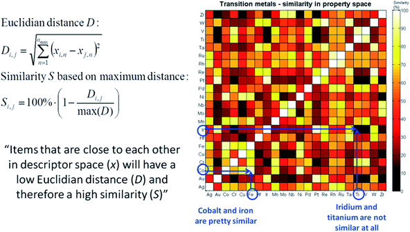Fig. 16 Graphical representation and mathematical equations describing the concept of “similarity” in the descriptor space.

3.5. Extension to other classes of catalysts

In this work we largely focus on catalysts composed of metals or metal oxides supported on oxide carriers. The methodology used however is quite generic in nature and is readily extended to other classes of catalysts. Of course, each class of catalysts will have its own relevant subset of descriptors. Taking zeolites as an example, as a first pass one could consider using the Si–Al ratio, the pore size and the number, density and type of the acid sites present. When metals are used, either exchanged or impregnated, the descriptor set could be augmented with descriptors as those presented here. In the case of metal–organic frameworks (MOFs), the descriptor list could include the size and charge of the metal ions at the vertices, the dimensions and backbone flexibility of the connecting organic species, and the possibility for binding at the surface and in the pores (van der Waals forces, pi-stacking).^51,52 For supported ligand–metal complexes, the descriptors would include the strength and length of the binding (grafting) group to the surface, the ligand bind angle and Tolman's cone angle, the size of the reaction pocket (which is often correlated with the cone angle), and the concentration/dispersion of active sites on the surface.^53,54 But in all cases, the workflows shown in Fig. 1 and 17 will be similar, and the main principle of this tutorial, combining modelling and experimentation, will hold.

Fig. 17 Workflow for data-driven catalyst development. Note that the workflow is iterative in nature – several cycles will typically have to be completed before reaching the end of a development project.

4. Conclusions

Discovering and optimising solid catalysts is still largely an empirical business. But this process can be helped by using the right combination of experimental design, descriptor modelling, high-level modelling, and experimental feedback and validation. A successful optimisation workflow is per definition iterative, and should include all three capacities (statistical design, experimental testing capabilities, and descriptor modelling and validation; see example in Fig. 17). Integrating these capacities (and people!) in one team, and realising that multiple iterations are needed, are the keys to success. Furthermore, since much of the research on solid catalysts is done in industrial environment, budgeting for multiple iterations of experiments, modelling, and validation will help you create and manage realistic expectations.

Notes and references

1. S. Arndt, T. Otremba, U. Simon, M. Yildiz, H. Schubert and R. Schomaecker, Appl. Catal., A, 2012, 425–426, 53–61.
2. M. R. Lee, M.-J. Park, W. Jeon, J.-W. Choi, Y.-W. Suh and D. J. Suh, Fuel Process. Technol., 2012, 96, 175–182.
3. E. McFarland, Science, 2012, 338, 340–342.
4. Q. X. Zhang, W. J. Li, B. Zhang, J. R. Zhang and Z. X. Wang, Adv. Mater. Res., 2012, 361, 579–583.
5. S. B. Derouane-Abd Hamid, J. R. Anderson, I. Schmidt, C. Bouchy, C. J. H. Jacobsen and E. G. Derouane, Catal. Today, 2000, 63, 461–469.
6. M. Heintze and M. Magureanu, J. Catal., 2002, 206, 91–97.
7. S. Liu, L. Wang, R. Ohnishi and M. Ichikawa, J. Catal., 1999, 181, 175–188.
8. S. Jenner and A. J. Lamadrid, Energy Policy, 2013, 53, 442–453.
9. D. A. Wood, C. Nwaoha and B. F. Towler, J. Mol. Gas Sci. Eng., 2012, 9, 196–208.
10. F. Wang, M. Luo, W. Xiao, X. Cheng and Y. Long, Appl. Catal., A, 2011, 393, 161–170.
11. J. G. Zeikus, M. K. Jain and P. Elankovan, Appl. Microbiol. Biotechnol., 1999, 51, 545–552.
12. L. E. Manzer, Top. Catal., 2010, 53, 1193–1196.
13. A. Eerhart, A. P. C. Faaij and M. K. Patel, Energy Environ. Sci., 2012, 5, 6407–6422.
14. G.-J. M Gruter, L. Sipos and M. Adrianus Dam, Comb. Chem. High Throughput Screening, 2012, 15, 180–188.
15. T. C. R. Brennan, C. D. Turner, J. O. Kramer and L. K. Nielsen, Biotechnol. Bioeng., 2012, 109, 2513–2522.
16. P. T. de Souza Nascimento, A. P. P. L. Barbosa, A. Ishikawa, A. S. O. Yu and A. S. Camargo, Technology Management for Emerging Technologies (PICMET), Proceedings of PICMET'12, 2012.
17. J. A. Moulijn, M. Makkee, A. Wiersma and E. Van de Sandt, Catal. Today, 2000, 59, 221–230.
18. E.-J. Ras, in Catalytic Process Development for Renewable Materials, ed. J.-K. van der Waal and P. Imhof, Wiley-VCH, 2013.
19. K. Langfeld, B. Frank, V. E. Strempel, C. Berger-Karin, G. Weinberg, E. V. Kondratenko and R. Schomacker, Appl. Catal., A, 2012, 417, 145–152.
20. J. M. Cizeron, E. Scher, F. R. Zurcher, W. P. Schammel, G. Nyce, A. Rumplecker, J. McCormick, M. Alcid, J. Gamoras, D. Rosenberg and E.-J. Ras, US20130023709, 2013.
21. E.-J. Ras, M. J. Louwerse and G. Rothenberg, Catal. Sci. Technol., 2012, 2, 2456–2464.
22. E.-J. Ras, S. Maisuls, P. Haesakkers, G.-J. Gruter and G. Rothenberg, Adv. Synth. Catal., 2009, 351, 3175–3185.
23. E.-J. Ras, B. McKay and G. Rothenberg, Top. Catal., 2010, 53, 1202–1208.
24. E.-J. Ras, M. J. Louwerse, M. C. Mittelmeijer-Hazeleger and G. Rothenberg, Phys. Chem. Chem. Phys., 2013, 15, 8795–8804.
25. S. T. Sie, Rev. Chem. Eng., 1998, 14, 109–157.
26. S. T. Sie and R. Krishna, Rev. Chem. Eng., 1998, 14, 203–252.
27. G. Ertl, H. Knoezinger and J. Weitkamp, Preparation of solid catalysts, Wiley-VCH, 2008.
28. J. Regalbuto, Catalyst Preparation Science and Engineering, CRC Press, 2007.
29. R. D. Shannon and J. A. Pask, J. Am. Ceram. Soc., 1965, 48, 391–398.
30. V. Perrichon, A. Laachir, S. Abouarnadasse, O. Touret and G. Blanchard, Appl. Catal., A, 1995, 129, 69–82.
31. J. P. Boitiaux, J. Cosyns and S. Vasudevan, Appl. Catal., 1983, 6, 41–51.
32. N. Macleod, J. M. Keel and R. M. Lambert, Appl. Catal., A, 2004, 261, 37–46.
33. S. Gómez-Quero, T. Tsoufis, P. Rudolf, M. Makkee, F. Kapteijn and G. Rothenberg, Catal. Sci. Technol., 2013, 3, 962–971.
34. V. R. Calderone, N. R. Shiju, D. Curulla-Ferré and G. Rothenberg, Green Chem., 2011, 13, 1950–1959.
35. B. W. Hoffer, R. L. C. Bonné, A. D. van Langeveld, C. Griffiths, C. M. Lok and J. A. Moulijn, Fuel, 2004, 83, 1–8.
36. H. F. M. Boelens, D. Iron, J. A. Westerhuis and G. Rothenberg, Chem.–Eur. J., 2003, 9, 3876–3881.
37. P. Jonsson, A. I. Johansson, J. Gullberg, J. Trygg, B. Grung, S. Marklund, M. Sjöström, H. Antti and T. Moritz, Anal. Chem., 2005, 77, 5635–5642.
38. O. Trapp, J. Chromatogr., A, 2008, 1184, 160–190.
39. M. B. Kasiri, H. Aleboyeh and A. Aleboyeh, Environ. Sci. Technol., 2008, 42, 7970–7975.
40. J. Kansedo, K. T. Lee and S. Bhatia, Biomass Bioenergy, 2009, 33, 271–276.
41. E. Burello and G. Rothenberg, Int. J. Mol. Sci., 2006, 7, 375–404.
42. A. G. Maldonado and G. Rothenberg, Chem. Soc. Rev., 2010, 39, 1891–1902.
43. J. A. Hageman, J. A. Westerhuis, H.-W. Frühauf and G. Rothenberg, Adv. Synth. Catal., 2006, 348, 361–369.
44. N. Fey, J. Chem. Soc., Dalton Trans., 2010, 39, 296–310.
45. D. Farrusseng, C. Klanner, L. Baumes, M. Lengliz, C. Mirodatos and F. Schüth, QSAR Comb. Sci., 2005, 24, 78–93.
46. C. Klanner, D. Farrusseng, L. Baumes, M. Lengliz, C. Mirodatos and F. Schüth, Angew. Chem., Int. Ed., 2004, 43, 5347–5349.
47. B. Hammer and J. K. Nørskov, Adv. Catal., 2000, 45, 71–129.
48. L. S. Byskov, J. K. Nørskov, B. S. Clausen and H. Topsøe, J. Catal., 1999, 187, 109–122.
49. F. Besenbacher, I. Chorkendorff, B. S. Clausen, B. r. Hammer, A. M. Molenbroek, J. K. Nørskov and I. Stensgaard, Science, 1998, 279, 1913–1915.
50. J. K. Nørskov, T. Bligaard, J. Rossmeisl and C. H. Christensen, Nat. Chem., 2009, 1, 37–46.
51. J. C. Tan and A. K. Cheetham, Chem. Soc. Rev., 2011, 40, 1059–1080.
52. C. E. Wilmer, M. Leaf, C. Y. Lee, O. K. Farha, B. G. Hauser, J. T. Hupp and R. Q. Snurr, Nat. Chem., 2011, 4, 83–89.
53. J. M. Notestein and A. Katz, Chem.–Eur. J., 2006, 12, 3954–3965.
54. K. Köhler, R. G. Heidenreich, S. S. Soomro and S. S. Pröckl, Adv. Synth. Catal., 2008, 350, 2930–2936.

---