Taylor dispersion and the position-to-time conversion in microfluidic mixing devices
B.
Wunderlich
,
D.
Nettels
* and
B.
Schuler
*
Department of Biochemistry, University of Zurich, Winterthurerstr. 190, 8057 Zurich, Switzerland. E-mail: schuler@bioc.uzh.ch; nettels@bioc.uzh.ch; Fax: +41 44 635 5907; Tel: +41 44 635 5535
First published on 23rd October 2013
Abstract
Microfluidic mixing devices are increasingly popular tools for probing the non-equilibrium dynamics of biomolecular systems. Commonly, hydrodynamic focusing is used to reduce the length scales that limit the time of diffusive mixing in the laminar flow regime, such that even sub-millisecond dead times for triggering a reaction have been achieved. Detection of a suitable signal at different points along the channel downstream of the mixing region, corresponding to different times after mixing, then allows the kinetics of the reaction to be obtained. However, the requisite accurate conversion of the positions in the channel to times after mixing is complicated by Taylor dispersion, the combined effect of diffusion and shear flow on the dispersion of the molecules in the microfluidic device. As a result, an accurate position-to-time conversion has only been possible in the limiting regimes, i.e. for very early times, where sample diffusion can be neglected, and for very long times, where the molecules have uniformly sampled the entire channel cross-section. Here, we use detailed three-dimensional, time-dependent finite-element calculations to obtain an accurate position-to-time conversion that bridges these two limits and allows us to quantify the effects of Taylor dispersion on the time resolution of a representative mixing device optimized for single-molecule fluorescence detection. The accuracy of the calculations is confirmed by direct comparison of the calculated velocity field with dual-focus fluorescence correlation spectroscopy measurements.
Introduction
Microfluidic mixing1 has become a popular technique for studying the dynamics of chemical and biological systems. Of particular recent interest are the dynamics of biological macromolecules; examples include protein folding,2–17 RNA folding,18,19 or biomolecular interactions.14,20 Advantages of microfluidic mixing over traditional methods for triggering such reactions can be access to shorter mixing times, lower sample consumption, reduced optical path length, or the suitability for interfacing with optical detection systems, such as confocal single-molecule spectroscopy. Owing to the low Reynolds numbers characteristic of microfluidic devices, flow in these systems is laminar, and turbulence cannot be used to enhance mixing.21 A simple and elegant method is to reduce the distances of diffusive mixing by hydrodynamic focusing,22 where a central fluid jet is confined by an outer flow in a narrow channel (Fig. 1a). As a result, diffusive exchange of molecules between the neighbouring streams is sufficiently fast for dead times of several microseconds to be achievable.6,23 The mixing time is then determined essentially by the translational diffusion coefficient, D, of the molecules to be mixed and the lateral dimensions of the channel.22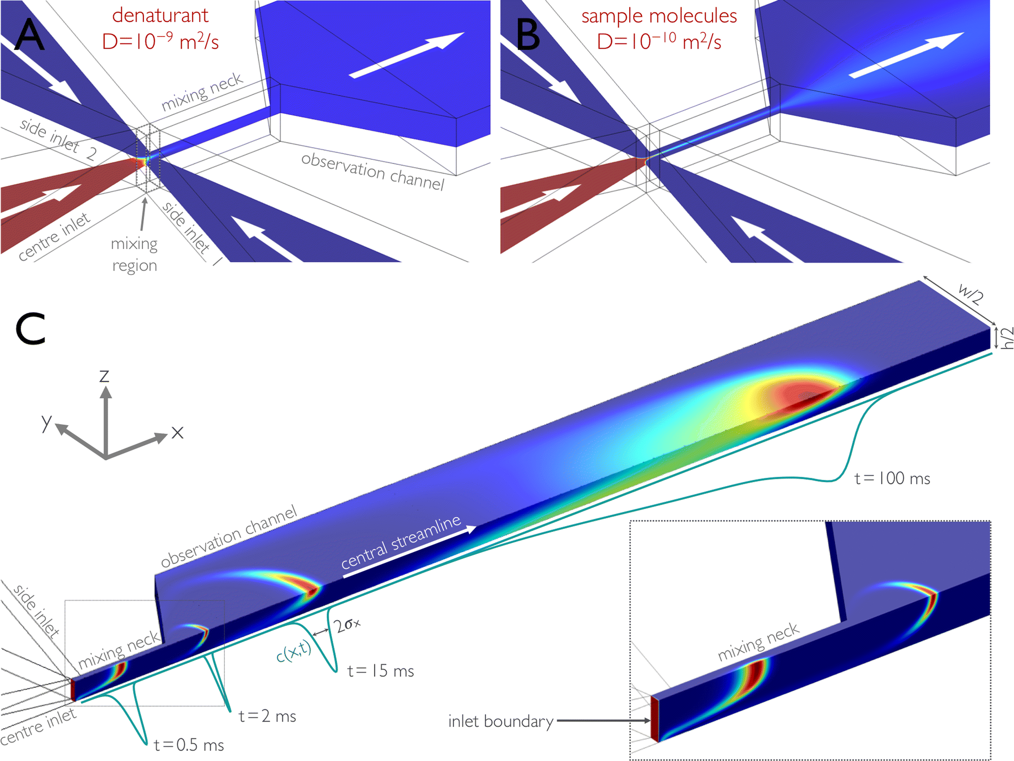 | ||
Fig. 1 Illustration of microfluidic mixing based on finite element calculations. In a typical experiment, sample molecules in high concentrations of denaturant are supplied from the centre inlet and mixed at a 1![[thin space (1/6-em)]](https://www.rsc.org/images/entities/char_2009.gif) :10 ratio with buffer without denaturant from the side channels. The concentration of solutes is indicated by a colour scale and decreases from red to blue. (A, B) The concentration distribution of molecules with two different diffusion constants is shown on a cut plane of a 3D finite-element calculation for molecules with a high diffusion constant (D = 10−9 m2 s−1), e.g. denaturant molecules (A), and with a low diffusion constant (D = 10−10 m2 s−1), e.g. sample molecules such as proteins (B). For a given set of driving pressures corresponding to an average flow velocity in the observation channel of 1.0 mm s−1, mixing due to diffusion for small solutes, such as denaturants, is complete by the end of the narrow mixing neck, and the concentration of the denaturant is uniform in the observation channel (A). In contrast, sample molecules with a lower diffusion constant remain hydrodynamically focused to a thin jet and disperse across the channel on a much longer timescale (B). (C) Impulse response of the microfluidic mixing device, calculated for obtaining the position-to-time conversion and its uncertainty. Only one quadrant of the device is shown. A 0.01 ms Gaussian pulse of sample molecules (D = 10−10 m2 s−1) is released from the centre inlet, and its propagation is modelled using 3D time-dependent finite-element calculations. An overlay of four (normalized) snapshots of the finite-element calculations at 0.5, 2, 15, and 100 ms after release of the pulse is shown. The inset shows a blow-up of the concentration profiles in the mixing neck at 0, 0.5, and 2 ms after release of the pulse. The concentration as a function of the position along the central streamline, c(x,t), is derived from the snapshots and shown as (normalized) propagating peaks (cyan lines). For each snapshot, we calculated from c(x,t) the standard deviation σx(t) of the distribution (Fig. 3). For determining the position-to-time conversion and its uncertainty (Fig. 4), we calculated for each position x from c(x,t) the mean arrival time after mixing, 〈t〉(x), and the standard deviation of this distribution, σt(x). :10 ratio with buffer without denaturant from the side channels. The concentration of solutes is indicated by a colour scale and decreases from red to blue. (A, B) The concentration distribution of molecules with two different diffusion constants is shown on a cut plane of a 3D finite-element calculation for molecules with a high diffusion constant (D = 10−9 m2 s−1), e.g. denaturant molecules (A), and with a low diffusion constant (D = 10−10 m2 s−1), e.g. sample molecules such as proteins (B). For a given set of driving pressures corresponding to an average flow velocity in the observation channel of 1.0 mm s−1, mixing due to diffusion for small solutes, such as denaturants, is complete by the end of the narrow mixing neck, and the concentration of the denaturant is uniform in the observation channel (A). In contrast, sample molecules with a lower diffusion constant remain hydrodynamically focused to a thin jet and disperse across the channel on a much longer timescale (B). (C) Impulse response of the microfluidic mixing device, calculated for obtaining the position-to-time conversion and its uncertainty. Only one quadrant of the device is shown. A 0.01 ms Gaussian pulse of sample molecules (D = 10−10 m2 s−1) is released from the centre inlet, and its propagation is modelled using 3D time-dependent finite-element calculations. An overlay of four (normalized) snapshots of the finite-element calculations at 0.5, 2, 15, and 100 ms after release of the pulse is shown. The inset shows a blow-up of the concentration profiles in the mixing neck at 0, 0.5, and 2 ms after release of the pulse. The concentration as a function of the position along the central streamline, c(x,t), is derived from the snapshots and shown as (normalized) propagating peaks (cyan lines). For each snapshot, we calculated from c(x,t) the standard deviation σx(t) of the distribution (Fig. 3). For determining the position-to-time conversion and its uncertainty (Fig. 4), we calculated for each position x from c(x,t) the mean arrival time after mixing, 〈t〉(x), and the standard deviation of this distribution, σt(x). | ||
After mixing, the sample is typically probed at different positions along an observation channel that follows the mixing region, corresponding to different times after the start of the reaction. The reaction kinetics can then be reconstructed from a series of these measurements. However, to obtain the correct kinetics, the positions need to be converted accurately to times after mixing. This position-to-time conversion is easily done for very short times, where diffusion of the sample molecules is negligible, and for very long times, where the molecules have uniformly sampled the entire channel cross-section. For intermediate times, however, such a conversion is not easily accessible. Here, we show how an accurate position-to-time conversion can be obtained from three-dimensional, time-dependent finite-element calculations. A key aspect for quantifying the behaviour of microfluidic mixing devices is the relative role of diffusion and advection, as detailed in the following sections.
Many applications of microfluidic mixing involve solutes of different sizes and thus of different translational diffusion coefficients. An example is protein folding, where the reaction is often triggered by rapidly changing the pH or diluting out a denaturant, such as urea or guanidinium chloride. In this case, diffusive mixing of the small solutes – and thus the start of the folding reaction – will be complete much earlier than a uniform distribution of the protein molecules across the channel is reached. This situation is illustrated in Fig. 1. An aqueous solution of denaturant and unfolded protein enters the mixing region through the centre inlet and is hydrodynamically focused by the buffer solutions entering from the side inlets. Mixing of the denaturant is complete by the time the solution has reached the end of the mixing neck (Fig. 1a),10,17 but the protein molecules (or sample molecules in general) are still confined to a thin jet (Fig. 1b). In other words, the difference in the relative importance of advection and diffusion (as expressed in the Péclet number, Pe) leads to different degrees of dispersion for the small solutes and the larger sample molecules. As a result, the sample molecules are not distributed evenly across the following observation channel (Fig. 1b), where the read-out of the experiment takes place.
In many cases, a uniform distribution of sample molecules across the observation channel is not strictly required, e.g. if the experimental observable is independent of sample concentration, or if the geometry is chosen in a way that the signal is integrated over all molecules at a certain distance from the mixing region. However, the difference in Péclet numbers for small solutes and larger sample molecules has an important consequence for defining the time axis of the reaction kinetics: while the sample molecules travel down the microfluidic channel, they diffuse in the plane of the channel cross-section (perpendicular to the flow) and visit streamlines with different flow velocities. As a consequence, the arrival time of each molecule at the point of observation depends on its individual three-dimensional trajectory through the channel. The resulting distribution of arrival times entails an intrinsic uncertainty in the conversion of the position in the observation channel to the time after mixing. The underlying phenomenon is well known in the field of fluid dynamics as Taylor dispersion (or Taylor–Aris dispersion)21,24–29 (Fig. 1c).
The importance of Taylor dispersion for microfluidic systems has long been recognized,21,29–40 but including it quantitatively in the position-to-time conversion of microfluidic mixing devices has been difficult. Only two limiting regimes have been easily accessible:21,30–33,36–39,41 for very early times after the mixing region, the diffusion of the sample molecules can be neglected, and the position in the observation channel can be converted to the time after mixing by simply using the flow velocity at the central streamline; for very late times, when the molecules have uniformly sampled the entire channel cross-section, the analytical steady-state solution for Taylor dispersion in the appropriate channel geometry29 can be used. However, for the intervening times, no analytical solution is available and an accurate position-to-time conversion has not been possible. The device investigated here, which was designed specifically for single-molecule fluorescence detection,10,17 is a case where the implications of this limitation are particularly severe: the two limiting regimes are only valid for times less than ~10 ms and above ~10 s, respectively. The largest part of the total accessible time range (from ~1 ms to ~1 min) is thus in the cross-over regime between the two limits, which has limited the accuracy of kinetic measurements with devices of this type.10,17
An additional aspect that has received very little attention to date is the effect of Taylor dispersion on the uncertainty of the times obtained from a given position-to-time conversion, i.e., the time resolution of the mixer. One possible reason for this neglect is that other uncertainties have been considered dominant, e.g. imperfections in channel fabrication or flow regulation. However, as illustrated in Fig. 2 and discussed in more detail below, even microfluidic devices produced by replica moulding with silicone elastomers can now be fabricated routinely with high accuracy and operated at the designed specifications. Under these circumstances, Taylor dispersion does become an important factor to take into account for the quantitative use of microfluidic mixing devices. Here, we thus take the example of a well-characterized microfluidic mixing device10,17 to quantify the effect of Taylor dispersion on the position-to-time conversion and the resulting time resolution based on three-dimensional (3D) finite-element calculations whose accuracy is referenced by direct comparison to experimental data.
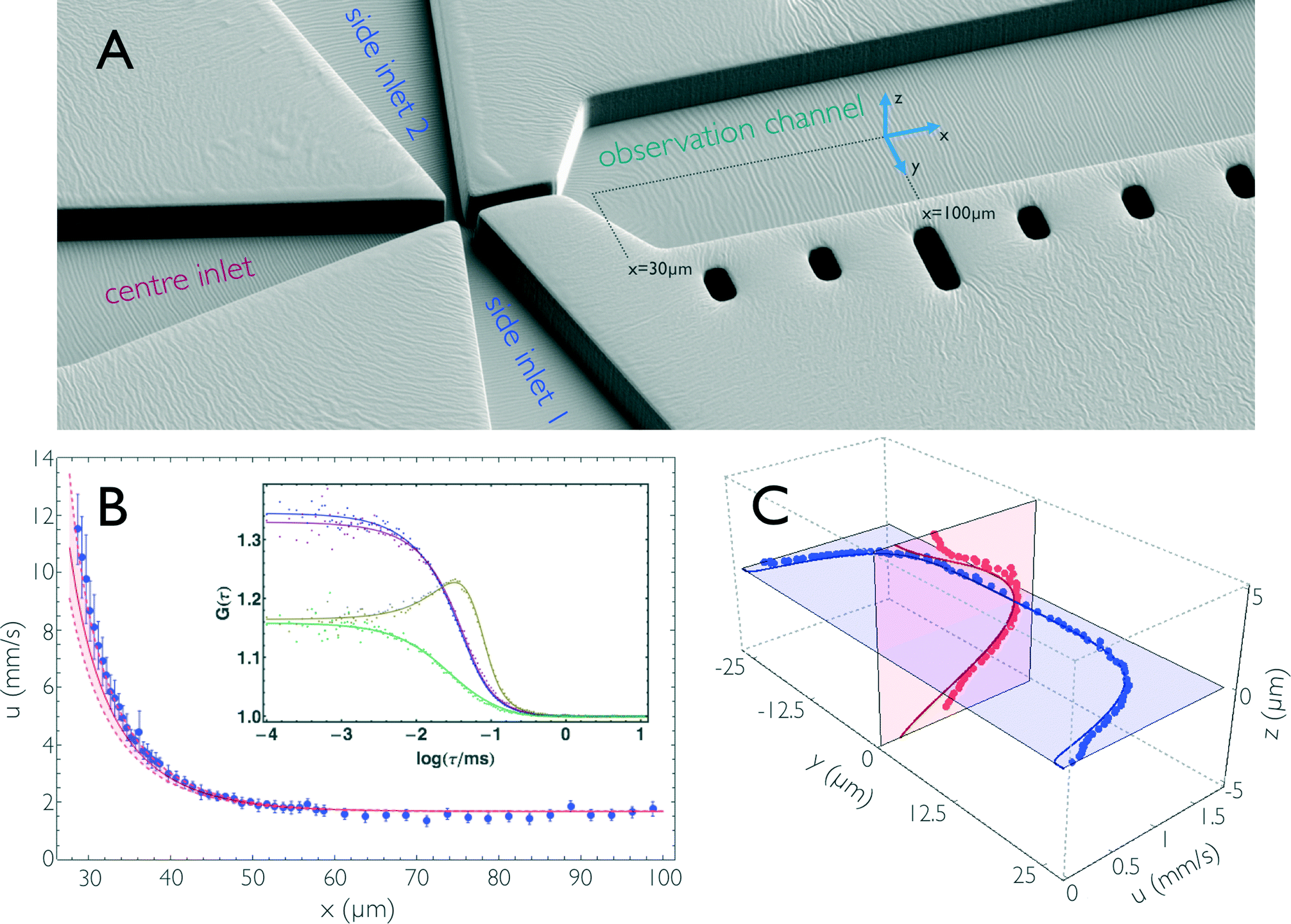 | ||
| Fig. 2 (A) Electron micrograph of the mixing region of the microfluidic device (PDMS coated with 5 nm platinum) showing the fabricated structures in an orientation similar to that of Fig. 1a and b. (B) Flow velocity, u, along the central streamline in the hydrodynamic entrance length. Blue dots are flow velocities derived from dual-focus FCS measurements; error bars indicate standard deviations estimated from three measurements. The red line is the result from 3D finite-element calculations, with an uncertainty estimated by assuming an uncertainty of ±1 μm in the position of the confocal volumes along x (shown as dashed lines). The inset shows representative correlation curves of the dual-focus FCS measurements, recorded at x = 29.25 μm. (x = 0 is at the centre of the mixing region.) The two auto- (blue and violet) and the two cross-correlations (yellow and green) of the two foci are shown with a global fit taking into account both diffusive and advective contributions to the correlation functions.32 (C) Flow velocity measurements across the observation channel. Dual-focus FCS measurements were performed on the mid-planes of the microfluidic chip at x = 100 μm. Blue and red dots are measured data, and blue and red lines are the corresponding results from finite-element calculations. The calculated values are corrected for the finite size of the confocal volume (see Materials and methods). | ||
Materials and methods
Device fabrication and operation
A detailed description of the fabrication process has been published previously.10,17 Briefly, microfluidic mixing devices are fabricated by replica moulding in PDMS. Silicon master moulds are structured using photolithography and deep reactive ion etching to a height of 10 μm, as confirmed by surface profiling. Inlets are punched into the 25 × 25 mm PDMS devices, which are bound to fused silica cover slides after plasma activation. Assembled microfluidic mixing devices are mounted in a custom-built cartridge system and loaded into a temperature-controlled holder. Pressure-driven flow is exerted via electro-pneumatic pressure controllers.17Dual-focus-FCS measurements
Dual-focus-FCS measurements were performed on a confocal single-molecule instrument (MT200, PicoQuant), equipped with two diode lasers (LDH-P-C-485, PicoQuant) for the interleaved generation of orthogonally polarized laser pulses at 485 nm. Both lasers were driven at 20 MHz repetition rate by a multichannel driver (Sepia II, PicoQuant) with a laser power of 30 μW, measured at the back aperture of the 1.2 NA, 60× microscope objective (UplanApo 60/1.20W Olympus). The objective is mounted on a piezo stage combination (P-733.2 and PIFOC, PI), which allows precise positioning of the laser foci inside the observation channel. The two foci are generated with the help of a differential interference contrast (DIC) prism (U-DICTHC, Olympus). The distance d = 420 ± 10 nm between the foci in aqueous solution was determined by measuring a series of reference samples of known diffusion coefficient.42 Fluorescence photons, collected by the objective, are focused on a 150 μm pinhole before being randomly distributed by a 50/50 beam splitter on two single-photon avalanche photodiodes (tau-SPAD 50, PicoQuant) after passage of a band-pass filter (ET525/50M, Chroma Technology). The photon detection times were recorded by two channels of a HydraHarp 400 counting module (PicoQuant), which was synchronized with the laser driver in order that excitation pulses and detected photons can be assigned to the individual foci. The fluorescence intensity cross- and autocorrelation curves obtained from the data of each focus were analysed using C++ and Mathematica (Wolfram Research) with an algorithm described by Arbour and Enderlein43 to obtain diffusion coefficients and flow velocities (Fig. 2b).For flow velocity measurements, 0.74 nM Alexa Fluor 488 dissolved in double-distilled water, containing 0.01% Tween 20, was first measured in a cuvette, i.e. in the absence of flow, to determine the translational diffusion coefficient. For the flow velocity measurements, the centre and side inlets of the microfluidic device were filled with the dye solution. The channel pressures were chosen to yield an average flow velocity of 1.0 mm s−1 in the observation channel and a mixing ratio of 1:10.17 The laser foci were placed at defined positions inside the observation channel, and the fluorescence signal was recorded for one minute at each position. Flow velocities were quantified from the analysis of the dual-focus-FCS data with the value of the diffusion coefficient constrained to the value in the absence of flow. Dual-focus-FCS allows the three-dimensional flow velocity vector to be obtained.43 Only the component in channel direction, the x-component, proved to be significantly different from zero under pressure-driven flow with proper alignment of microfluidic device and detection system. Note that the measured velocities are limited in spatial resolution due to the finite dimensions of the foci. For the comparison of the calculated velocity profiles with the experimental results (Fig. 2c), the calculated profiles were convolved with the corresponding shape of the foci. Confocal imaging of fluorescent beads (SpectraBeads, 200 nm diameter) immobilized on a cover-slide showed that each focus is roughly shaped like a prolate ellipsoid and can be approximated by a 3D Gaussian distribution of ~2.6 μm in height (along z) and ~0.6 μm in diameter (along x and y; the values refer to an intensity drop of 1/e2).
Finite-element calculations
Finite-element calculations were performed using COMSOL Multiphysics 4.3a. Only one quadrant of the mixing device needed to be modelled. Owing to its geometry (rectangular channel cross-sections, cuboidal mixing region, and orthogonal crossing of the four channels), a hexahedral meshing was used to obtain accurate and time-efficient calculations. The channel parts with constant cross-section were modelled with cuboidal elements; the connecting segments with narrowing or widening channel widths were modelled with parallelepipeds. Technically, the mesh is generated by “sweeping” the cross-sectional mesh, defined at one boundary, along the channels. The cross-sectional mesh was built from 25 × 10 elements distributed along the half width and half height of the channels. Two different distributions of elements were used. For the flow velocity calculations, the mesh resolution was increased towards the channel walls to accurately map the steep velocity gradient near the walls. In axial direction (along x), the mesh separation started with 0.25 μm in the mixing region and increased towards the inlet and observation channels, up to 2 mm into the regions where the flow profile is constant in axial direction. For the impulse response calculations, the lateral mesh separation was equidistant across the channel. In axial direction, a particularly fine mesh was needed in the region where the pulse is still very narrow (mesh separation ~0.1 μm), whereas the other regions of the mixing device could be modelled with much less resolution (mesh separation up to 100 μm near the outlet boundary). We calculated the pulse propagation separately for five consecutive time intervals with different meshes optimized for each interval: from 0–0.5 ms, the initial phase of release of the concentration pulse; from 0.5–2.5 ms, corresponding to the early entrance length with a strong decrease in flow velocity in axial direction; from 2.5–25 ms, when the pulse propagates in fully developed flow; from 25–500 ms, the region where the molecules sample streamlines with different flow velocities predominantly along the z-axis; and from 0.5–70 s, where the molecules approach uniform sampling of the cross-section. The final concentration distribution of each interval was used as the initial distribution for the following one.The COMSOL Multiphysics' “creeping flow” package was used for calculating the stationary flow velocity distribution and the “transport of diluted species” package was used for the impulse response calculation. In the latter case, the “segregated solver” was used, with a lower limit for the concentration set to zero to avoid artificial negative concentrations. The “backward differentiation formula (BDF)” time-stepping method of COMSOL Multiphysics was used with at least one time step (“intermediate” setting) between predefined intervals of the time-dependent finite-element calculations. 0.01 ms intervals were chosen for times up to 2.5 ms, and then the intervals were gradually increased, with the maximum step size of the time-dependent solver set to 10 ms. Calculations were performed on a dual Intel Xeon server with six cores and hyperthreading, equipped with 64 GB of RAM. Owing to the fine mesh required, typical calculations of the impulse response required ~2–3 days for one set of parameters.
Results and discussion
Device geometry and design
The mixing device used here has been employed for a range of questions, especially regarding conformational changes and folding of proteins.11,15–17 The solution containing the macromolecule of interest is introduced via the centre inlet and is hydrodynamically focused to a thin jet by the fluid from the two side channels (Fig. 1A). In the narrow mixing neck (width 2.5 μm), diffusion of small solutes across the channel and between the fluid layers leads to a rapid change in solution conditions and triggers the reaction within ~1 ms (e.g. the folding or unfolding of a protein by a decrease or increase in denaturant concentration).17 In the following broad observation channel (width 50 μm), the flow velocity is reduced to an average value of 1.0 mm s−1 in order to reach residence times of the individual molecules in the micrometre-sized confocal observation volume that are sufficiently long for single-molecule detection. The large width of the observation channel also optimizes the photon collection efficiency by accommodating the entire excitation and fluorescence collection cones of the high numerical aperture objectives used in confocal single-molecule spectroscopy.10 To allow kinetics to be recorded on timescales up to minutes, most of the downstream part of the observation channel is folded in a serpentine shape,17 resulting in a total length of 62 mm. With a channel depth of 10 μm, the Reynolds number for the device is on the order of 10−2, ensuring completely laminar flow under all conditions used here. The device is optimized for a mixing ratio of 1:10, but can be operated reliably in a range of mixing ratios from about 1:20 to 1:5.17 Silicon masters fabricated by reactive ion etching are used for replica moulding with polydimethylsiloxane (PDMS). The resulting devices (Fig. 2a) are plasma-bonded to microscope cover slides and mounted on the single-molecule instrument as described previously.17
Stationary flow velocity
The stationary flow velocity in the device channels, u(r), was calculated by solving the Stokes equations for an incompressible Newtonian fluid:44 ∇p = μ∇2u and ∇·u = 0, where ∇p is the pressure gradient and μ is the dynamic viscosity of the solvent. The pressure differences between inlet and outlet channels are chosen in order that a mixing ratio of R = 1:10 and a mean flow velocity in the observation channel of 1.0 mm s−1 are obtained. The values can be calculated using a simple lumped-impedance model of the mixer.10,17 For μ = 1 mPa s, we obtain pcenter = 15.1 kPa, pside = 16.0 kPa, and pobs = 0 kPa. Here we assume that the viscosity is constant throughout the device. In practice, the solvents in the inlets can differ in viscosity. Note, however, that the mixing of the solvents is completed in the mixing neck, and the viscosity is homogeneous afterwards, i.e. the velocity field in the observation channel is independent of the viscosity differences in the inlet channels.
The Stokes equations are solved with a no-slip boundary condition (u = 0) at the channel walls. The microfluidic device was modelled in 3D using finite-element calculations (COMSOL 4.3a). Owing to the symmetry of the device in the xy- and xz-planes, the calculations could be reduced to only one quadrant of the microfluidic device (see Fig. 1c). For simplicity, the observation channel was modelled as a straight, 62 mm long channel of rectangular cross-section with height h and width w (h/2 = 5 μm, w/2 = 25 μm), i.e., the details of the flow in the turns of the serpentine-shaped part of the observation channel were neglected. In the following section, we discuss only the flow velocity component parallel to the channel axis, u(r) = ux(r).
An important prerequisite for using finite element methods to obtain the position-to-time conversion (see Impulse response) is to ensure quantitative agreement of the calculations with the experimentally observed properties of the flow. We thus directly compared the flow velocities obtained from finite-element calculations with those from dual-focus-FCS measurements43,45 (Fig. 2b and c). With dual-focus-FCS, precise and accurate velocity information is obtained from cross- and autocorrelations of the fluorescence intensities emitted from two confocal observation volumes of known separation (here, d = 420 ± 10 nm) positioned on a line parallel to the channel axis43 (Fig. 2b). For comparison with the experimental data, we convolved the calculated flow velocities u(r) in the yz-plane with a 2D Gaussian of dimensions corresponding to the confocal volume (see Materials and methods for details). The convolution along the x coordinate was neglected because the velocity gradient is shallow in the x-direction, except for the very beginning of the observation channel. The flow velocity along the central streamline, starting from the beginning of the observation channel (x ≈ 30 μm) to position x ≈ 100 μm, is depicted in Fig 2b. (Note that x = 0 is at the centre of the mixing region [Fig. 1a].) We observe how the flow velocity along this streamline drops to a final value of u = 1.68 mm s−1 after exiting the narrow mixing channel. Fig. 2c shows the vertical and horizontal flow velocity profiles along the planes intersecting at the centre of the observation channel at position x = 100 μm, where the flow is fully developed. In the vertical direction (z-axis), the velocity profile is approximately parabolic, whereas the horizontal profile is flattened, and the velocity decreases only close to the sidewalls of the channel, as expected for a 10 μm × 50 μm rectangular cross-section. The deviations of the dual-focus-FCS data from the calculated data near the channel walls are most probably caused by distortions of the confocal volume at the PDMS/solvent interfaces. Overall, we observe excellent agreement of the flow velocity field from finite-element calculations and experiment, not only with respect to the trends, but also for the absolute flow velocities. This finding shows that the finite-element calculations provide an accurate and precise representation of the fluid dynamics in the microfluidic mixing device, which enables us to use the calculations for obtaining a position-to-time conversion by including the diffusivity of the sample molecules and the time dependence of the convective processes in the device.
Stationary sample and solvent concentrations
In the next step, u(r) from the stationary flow velocity calculations was used to solve the advection-diffusion equation,29,44| ∂tc(r,t) = D∇2c(r,t) − u(r)·∇c(r,t) | (1) |
Impulse response
The key aspect of our work is to investigate the effect of Taylor dispersion on the position-to-time conversion and the time resolution of microfluidic mixing. This step requires us to quantify the time-dependent interplay of diffusion and advection on the dispersion of sample molecules as they travel down the microfluidic device.24,25,27,29 Based on the quantitative agreement between the calculated and observed velocity fields in the chip (Fig. 2), we can use the time-dependent form of eqn (1) as implemented in COMSOL Multiphysics to calculate the propagation of a short pulse of sample molecules emitted from the boundary surface at the very end of the centre inlet channel (Fig. 1c, inset). The calculated dispersion of the pulse along the channel can then be analysed to obtain the position-to-time conversion and the resulting uncertainties in the arrival times of molecules at the point of observation. The initial pulse is Gaussian-shaped in time (standard deviation 0.01 ms), but spatially uniform across the inlet boundary, thus resembling a thin layer of a high concentration of sample molecules, which then propagates along the channel. We define the point in time when the centre of the distribution has reached the centre of the mixing region (Fig. 1a) as the time origin or time of mixing, t = 0. The pulse propagation through the observation channel was calculated for times up to 70 s. Snapshots of the resulting concentration distributions were calculated at 10 μs intervals for short times (up to 2.5 ms) and at increasingly longer intervals of up to 0.5 s for 50 s to 70 s.Fig. 1c shows the propagated pulse at several different times in the mixing neck and in the observation channel. The blue lines represent the concentration distribution, c(x,t), along the central streamline. In the mixing neck, the molecules get hydrodynamically focused in the y-direction, whereas pronounced advective stretching occurs in the xz-plane, followed by deceleration of the flow during entry in the observation channel. As a result, the sample concentration exhibits a narrow peak close to the channel centre at the beginning of the observation channel. With the lower average flow velocity, the Péclet number drops, and diffusive motion transports more of the molecules towards the channel walls, where they fall behind the other molecules due to the lower flow velocity in this region. The concentration distribution becomes parabolic in shape along both y and z, but the distribution along the central stream line is still quite symmetric and narrow for early times. At longer times, however, the molecules have sampled the channel cross-section more extensively, which results in a broad distribution of distances travelled since t = 0. The concentration distribution along the central stream line is correspondingly broad and highly asymmetric (Fig. 1c). It is this broad distribution caused by Taylor dispersion that needs to be taken into account for converting the position in the observation channel to the time after mixing.
The concentration distribution along the central streamline
In typical mixing experiments with single-molecule spectroscopy, we collect only the fluorescence emitted from the confocal volume (~1 μm3) of the microscope, which is positioned at the centre of the observation channel cross-section at different positions, x, along the channel. For the following analysis, we thus consider only the time and position dependence of the concentration distribution, c(x,t), along the central streamline (see the blue lines in Fig. 1c). For each time, t, we calculated the mean value, 〈x〉, and the mean square deviation, σ2x of the distribution along x. In the absence of Taylor dispersion, i.e. for a constant and uniform flow velocity in the entire channel, σ2x would increase in time solely due to diffusion according to σ2x = 2Dt. To illustrate the quantitative effect of Taylor dispersion on the effective diffusion coefficient, or dispersivity, we show in Fig. 3 the time derivative α(t) = dσ2x/dt in units of 2D as a function of the time after mixing. In this example, we use a value of D = 10−10 m2 s−1, a value corresponding to a protein of ~20 kDa molecular mass.46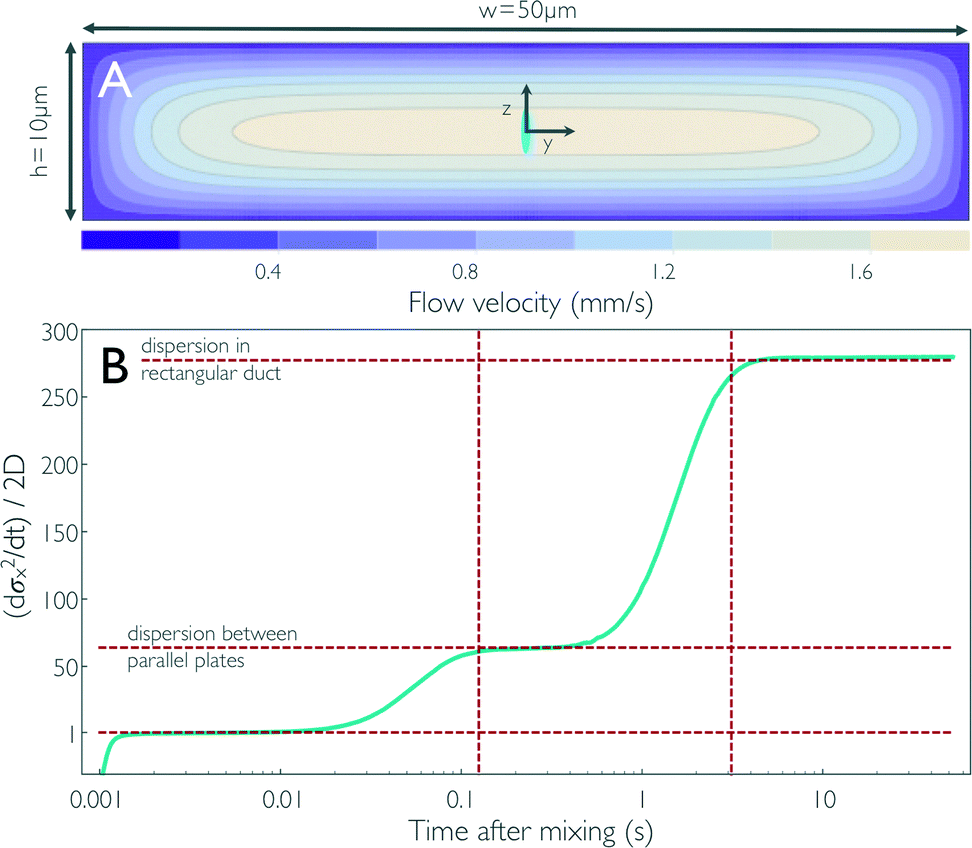 | ||
| Fig. 3 (A) Contour plot of the flow velocity profile in the cross-section of the observation channel for fully developed flow derived from 3D finite-element calculations. The size of the confocal volume placed on the central streamline is illustrated by the blue ellipse (corresponds to the 1/e2 contour). Diffusion of a particle from the central streamline to the top and bottom of the observation channel, corresponding to dispersion between flat plates, and to the sidewalls, corresponding to dispersion in a rectangular duct, takes on the order of 125 ms and 3.13 s, respectively, for D = 10−10 m2 s−1 (vertical dashed lines in B). (B) The time derivative of the standard deviation of the concentration distribution along x, which corresponds to an effective diffusion coefficient or dispersivity (cyan line), is shown as obtained from the impulse response calculations (Fig. 1c). The concentration pulse from the sample channel is first stretched as it enters the narrow mixing neck because of the large acceleration of the flow. As the pulse enters the observation channel, the flow velocity is reduced and the pulse is compressed again, which results in a negative dispersivity in the first millisecond after mixing. For times on the order of tens of milliseconds after mixing, the broadening of the pulse corresponds to dispersivity on the order of the diffusion coefficient of the sample molecule [(dσx2/dt)/2D ≈ 1]. The molecules then start sampling streamlines with lower flow velocities than the central streamline, and the broadening of the pulse results in a dispersivity ~63 times increased for times >0.1 s. Once the molecules are uniformly distributed across the channel cross-section, i.e. they diffusively sample streamlines near the sidewalls of the channel, a dispersivity of ~278 times the diffusion coefficient of the protein is reached. The values corresponding to (dσx2/dt)/2D = 1 and the dispersivities from Taylor dispersion for flow between two infinite parallel plates [(dσx2/dt)/2D = 64] and in a rectangular duct of the dimensions in (A) [(dσx2/dt)/2D = 277] are shown as horizontal dashed lines. | ||
Starting from the end of the mixing neck, we observe an increase of α in three steps (Fig. 3b): up to ~2 ms (x ≈ 35 μm), the strong negative velocity gradient along the x-axis (see Fig. 2b) dominates over diffusive broadening and leads to a compression of the distribution, corresponding to α < 0. During the following passage of the entrance length of the observation channel (2 ms < t < 10 ms), the deceleration along x levels off, but the sample molecules have diffused away from the central axis only very little; they are thus still predominantly located in a region where the velocity distribution across the channel cross-section is relatively flat, and α crosses zero and plateaus at a value close to unity. 10 ms has been altered for clarity, please check that the meaning is correct.?>For t > 10 ms, the molecules start to diffusively sample regions close to the upper and lower channel walls, where the flow velocity falls off strongly (see Fig. 3a), and we thus observe a first pronounced increase in α owing to Taylor dispersion. The increase levels off at ~100 ms to a value of α ≈ 62; on this timescale and above, essentially uniform diffusive sampling of the 10 μm height of the channel occurs. At t ≈ 1 s, α starts increasing in another step to a plateau at α ≈ 278, owing to diffusive sampling of the velocity field along the 50 μm width of the channel. For t > 5 s, α remains constant, indicating that the further increase in σx2 can be described by a constant effective diffusion coefficient, or the dispersivity, K = Dα. In this range, the concentration distribution along x regains a symmetric shape.
How do the α values we obtained from the finite-element results compare to calculations of the effect of Taylor dispersion in simple geometries? Commonly, α is expressed as:29
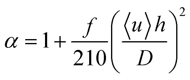 | (2) |
Position-to-time conversion and time resolution of the mixer
Finally, we can thus use the results from the impulse response calculations to obtain the position-to-time conversion for measurements in the microfluidic mixer and to quantify the uncertainty resulting from Taylor dispersion. In an experiment, the fluorescence signal of the sample is recorded by positioning the confocal observation volume at different positions, x, along the central streamline to obtain information about the kinetics of the system under study. Ideally, we would want all sample molecules to arrive at x at the same time after leaving the mixing region. In reality, however, the arrival times, t, for a given x are distributed according to c(x,t), the impulse response function. Analogous to the previous section, we can calculate from c(x,t) for each x the mean arrival time after mixing, 〈t〉(x), and σt(x). 〈t〉(x) is essential for converting the position of observation in the device to the mean time after mixing, and σt(x) provides a measure for the time resolution of our measurements.Fig. 4a shows 〈t〉(x) obtained from the finite element calculations together with the arrival times expected in two limiting cases: (1) if we assume for the position-to-time conversion the velocity along the central streamline, or (2) if we assume the average flow velocity of the fully developed flow in the observation channel. As expected from Fig. 1c and 3b, positions along x close to the mixing region are better approximated by limit (1) because, up to this point, diffusive exchange of molecules between the central streamline and peripheral regions of the channel with lower flow velocity is negligible. At positions further downstream from the mixing region, limit (2) is approached as the molecules increasingly sample the entire channel cross-section by diffusion. At intermediate positions, a cross-over between these two regimes is observed, and the position-to-time conversion depends on the diffusion coefficient of the sample molecules: the larger the diffusion coefficient is, the earlier limit (2) is approached. Fig. 4a illustrates this behaviour for sample molecules of three different diffusion coefficients, with values close to those of a typical fluorophore used in single-molecule detection (5.0 × 10⁻¹⁰ m2 s−1), a small protein (1.0 × 10⁻¹⁰ m2 s−1), and a large protein complex (2.5 × 10⁻¹¹ m2 s−1).
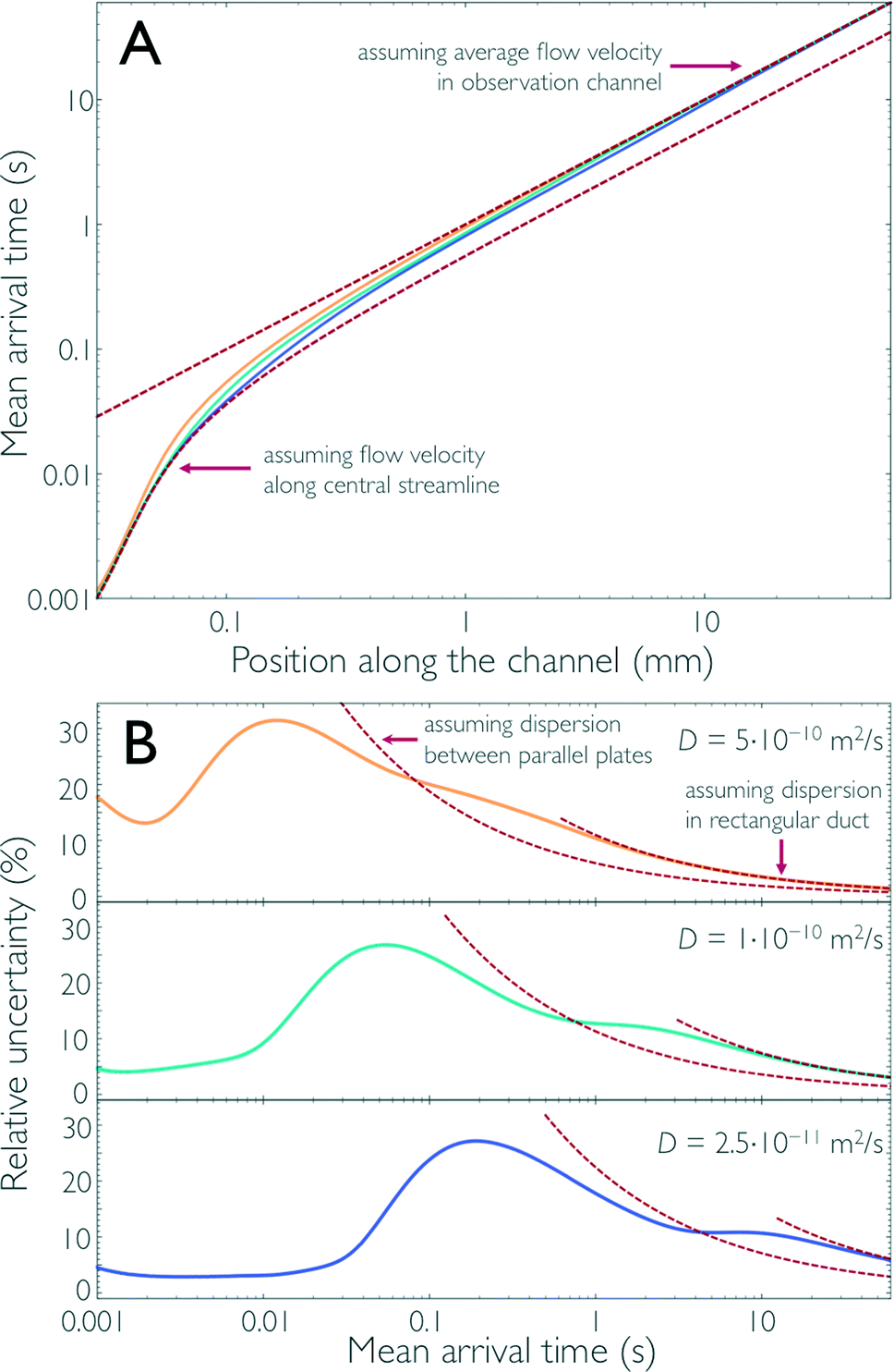 | ||
| Fig. 4 The results of the 3D finite-element calculations for the impulse response (Fig. 1c) can be used to determine the conversion for each position along the channel to the corresponding time after mixing, the position-to-time conversion of the mixing device. Both the mean arrival time 〈t〉 (A) and its relative uncertainty σt/〈t〉 (B) along the central streamline are shown for sample molecules with three different diffusion coefficients (5.0 × 10⁻¹⁰ m2 s−1, yellow; 1.0 × 10⁻¹⁰ m2 s−1, cyan; and 2.5 × 10⁻¹¹ m2 s−1, blue). For short times after mixing, the molecules have not sampled other streamlines and the time after mixing can essentially be derived from the flow velocity along the central streamline (lower dashed line in A). As the molecules start sampling other streamlines, the mean arrival time deviates from this line and approaches the arrival times assuming the average flow velocity in the observation channel (upper dashed line in A). Correspondingly, the relative uncertainty, as a function of the mean arrival time, is small for short times after mixing (B) but increases at intermediate times. For long times after mixing, when the concentration of the sample molecules is uniformly distributed across the cross-section of the observation channel, the uncertainty in the arrival time can be derived using Taylor dispersion in a rectangular duct (right red dashed lines in B). In the range of times where diffusive sampling of only the channel height is complete, the change in relative uncertainty is close to the behavior expected for Taylor dispersion in flow between two parallel plates (left red dashed lines in B). | ||
In Fig. 4b, we show, for the same three cases, σt/〈t〉 as a measure for the relative uncertainty in the arrival time, i.e. the time resolution of the measurement, at a given position x. Analogous to the discussion above for limit (1), the relative uncertainty in arrival times is small for 〈t〉 in the low millisecond range, especially for sample molecules with low diffusivity but exhibits a pronounced increase in the cross-over regime, to a maximum of ~30% for 〈t〉 between 10 and 200 ms, depending on the diffusion coefficient. For longer times, two characteristic decays in σt/〈t〉, which correspond to the plateau regions of α in Fig. 3b, are observed. Correspondingly, the changes in σt/〈t〉 are again close to the behaviour expected for two parallel plates and a rectangular duct with the dimensions of the observation channel, respectively (Fig. 4b). For long times, e.g. 〈t〉 > 5 s in the case of D = 10−10 m2 s−1, σt/〈t〉 drops below 10% and keeps decreasing, since in this regime the increase in dispersion along x according to eqn (2) is slower than the transport of the molecules along the channel with the average flow velocity. In other words, even though the absolute uncertainty in arrival time keeps increasing in this region approximately according to σt ∝  , the relative uncertainty, σt/〈t〉, is expected to decrease roughly with 〈t〉−1/2.†
Conclusions
Current microfabrication techniques allow the accurate production of microfluidic mixing devices with feature sizes down to a few micrometres, even with replica moulding. Uncertainties of kinetic measurements in these devices are thus no longer limited by imperfections in microfabrication, but by Taylor dispersion. The excellent agreement between the flow velocity profiles calculated with finite element methods and determined experimentally using dual-focus-FCS shown here justifies the use of computational fluid dynamics for calculating the position-to-time conversion for microfluidic mixers and the uncertainties owing to Taylor dispersion. Our impulse response calculations show that the dispersivity along the observation channel increases in two stages that correspond to the diffusive sampling of the short and long axes of the channel cross-section. The corresponding plateau values of the dispersivity are in good agreement with previous calculations for simple geometries, which supports the accuracy and convergence of the finite element approach. The impulse response calculations can thus be used to extract reliable position-to-time conversion functions, which allow every position along the channel to be assigned accurately to an average time after mixing, a crucial piece of information for determining reaction kinetics in microfluidic mixing experiments. Notably, the position-to-time conversion differs significantly from simple approximations that take into account only either the velocity along the central streamline (a reasonable approximation for very early times) or the average flow velocity in the channel (a reasonable approximation for long times), especially in the cross-over region between these two regimes. Calculations of the type presented here are thus indispensable for a fully quantitative analysis of microfluidic mixing experiments.Our results also show a significant effect of Taylor dispersion on the uncertainty in the mean arrival times of molecules at the point of observation, i.e. the time resolution of measurements. In the cross-over regime, relative uncertainties of up to ~30% are observed for the cases investigated here, an effect that needs to be taken into account for a quantitative analysis of the resulting kinetic data and their model-based interpretation. In single-molecule fluorescence experiments, e.g., the underlying distribution of times after mixing is expected to result in a broadening of the distributions of observables, such as transfer efficiencies or fluorescence lifetimes. However, if the correct position-to-time conversion is used and the uncertainties due to Taylor dispersion are taken into account, these effects will usually not preclude a quantitative kinetic analysis, especially since the larger uncertainties are limited to a relatively narrow range of observation times. Finally, we want to point out that the decrease in the relative uncertainty in the observed time after mixing according to σt/〈t〉 ∝ 〈t〉−1/2 for long times (>5 s in the case of D = 10−10 m2 s−1, corresponding to a typical small protein) allows the observation times to be extended much further than to the one-minute scale realized to date17 by simply extending the length of the observation channel. The scope of microfluidic mixing for a wide range of applications and timescales is thus likely to keep increasing. Time-dependent 3D finite-element calculations will be an important tool for taking full advantage of this potential.
Acknowledgements
We thank Dominik Hänni for help with sample preparation, Jörg Enderlein for providing his code for the analysis of dual-focus FCS measurements, Andrea Soranno and Hagen Hofmann for assistance with the calibration and analysis of dual-focus-FCS data, and Donat Scheiwiler und Stefan Blunier for helpful discussions. We also thank Everett Lipman, Shawn Pfeil, and Armin Hoffmann for discussions that led to the initiation of this investigation, and Hagen Hofmann and Stephan Benke for helpful comments on the manuscript. Electron microscopy was performed with support of the Centre for Microscopy and Image Analysis, University of Zurich, especially with the help of Andres Kaech. This work was supported by the Swiss National Science Foundation, the Swiss National Center of Competence in Research (NCCR) for Structural Biology, and a Starting Grant of the European Research Council.Notes and references
- J. M. Ottino and S. Wiggins, Philos. Trans. R. Soc., A, 2004, 362, 923 CrossRef PubMed.
- L. Pollack, M. W. Tate, N. C. Darnton, J. B. Knight, S. M. Gruner, W. A. Eaton and R. H. Austin, Proc. Natl. Acad. Sci. U. S. A., 1999, 96, 10115 CrossRef CAS.
- L. Pollack, M. W. Tate, A. C. Finnefrock, C. Kalidas, S. Trotter, N. C. Darnton, L. Lurio, R. H. Austin, C. A. Batt, S. M. Gruner and S. G. Mochrie, Phys. Rev. Lett., 2001, 86, 4962 CrossRef CAS.
- E. Kauffmann, N. C. Darnton, R. H. Austin, C. Batt and K. Gerwert, Proc. Natl. Acad. Sci. U. S. A., 2001, 98, 6646 CrossRef CAS PubMed.
- E. A. Lipman, B. Schuler, O. Bakajin and W. A. Eaton, Science, 2003, 301, 1233 CrossRef CAS PubMed.
- D. E. Hertzog, X. Michalet, M. Jager, X. X. Kong, J. G. Santiago, S. Weiss and O. Bakajin, Anal. Chem., 2004, 76, 7169 CrossRef CAS PubMed.
- A. Hoffmann, A. Kane, D. Nettels, D. E. Hertzog, P. Baumgärtel, J. Lengefeld, G. Reichardt, D. A. Horsley, R. Seckler, O. Bakajin and B. Schuler, Proc. Natl. Acad. Sci. U. S. A., 2007, 104, 105 CrossRef CAS PubMed.
- A. S. Kane, A. Hoffmann, P. Baumgärtel, R. Seckler, G. Reichardt, D. A. Horsley, B. Schuler and O. Bakajin, Anal. Chem., 2008, 80, 9534 CrossRef CAS PubMed.
- K. M. Hamadani and S. Weiss, Biophys. J., 2008, 95, 352 CrossRef CAS PubMed.
- S. H. Pfeil, C. E. Wickersham, A. Hoffmann and E. A. Lipman, Rev. Sci. Instrum., 2009, 80, 055105 CrossRef PubMed.
- H. Hofmann, F. Hillger, S. H. Pfeil, A. Hoffmann, D. Streich, D. Haenni, D. Nettels, E. A. Lipman and B. Schuler, Proc. Natl. Acad. Sci. U. S. A., 2010, 107, 11793 CrossRef CAS PubMed.
- Y. Gambin, C. Simonnet, V. VanDelinder, A. Deniz and A. Groisman, Lab Chip, 2010, 10, 598 RSC.
- S. A. Waldauer, O. Bakajin and L. J. Lapidus, Proc. Natl. Acad. Sci. U. S. A., 2010, 107, 13713 CrossRef CAS PubMed.
- Y. Gambin, V. Vandelinder, A. C. Ferreon, E. A. Lemke, A. Groisman and A. A. Deniz, Nat. Methods, 2011, 8, 239 CrossRef CAS PubMed.
- A. Borgia, B. G. Wensley, A. Soranno, D. Nettels, M. Borgia, A. Hoffmann, S. H. Pfeil, E. A. Lipman, J. Clarke and B. Schuler, Nat. Commun., 2012, 2, 1195 CrossRef PubMed.
- A. Soranno, B. Buchli, D. Nettels, S. Müller-Späth, R. R. Cheng, S. H. Pfeil, A. Hoffmann, E. A. Lipman, D. E. Makarov and B. Schuler, Proc. Natl. Acad. Sci. U. S. A., 2012, 109, 17800 CrossRef CAS PubMed.
- B. Wunderlich, D. Nettels, S. Benke, J. Clark, S. Weidner, H. Hofmann, S. H. Pfeil and B. Schuler, Nat. Protoc., 2013, 8, 1459 CrossRef CAS PubMed.
- R. Russell, I. S. Millettt, M. W. Tate, L. W. Kwok, B. Nakatani, S. M. Gruner, S. G. J. Mochrie, V. Pande, S. Doniach, D. Herschlag and L. Pollack, Proc. Natl. Acad. Sci. U. S. A., 2002, 99, 4266 CrossRef CAS PubMed.
- L. Pollack and S. Doniach in Methods in Enzymology: Biophysical, Chemical, and Functional Probes of Rna Structure, Interactions and Folding, Pt B, ed. Herschlag, D., Elsevier Academic Press Inc, San Diego, 2009, vol. 469, p. 253 Search PubMed.
- H. Y. Park, S. A. Kim, J. Korlach, E. Rhoades, L. W. Kwok, W. R. Zipfell, M. N. Waxham, W. W. Webb and L. Pollack, Proc. Natl. Acad. Sci. U. S. A., 2008, 105, 542 CrossRef CAS PubMed.
- T. M. Squires and S. R. Quake, Rev. Mod. Phys., 2005, 77, 977 CrossRef CAS.
- J. B. Knight, A. Vishwanath, J. P. Brody and R. H. Austin, Phys. Rev. Lett., 1998, 80, 3863 CrossRef CAS.
- H. Y. Park, X. Y. Qiu, E. Rhoades, J. Korlach, L. W. Kwok, W. R. Zipfel, W. W. Webb and L. Pollack, Anal. Chem., 2006, 78, 4465 CrossRef CAS PubMed.
- G. Taylor, Proc. R. Soc. London, Ser. A, 1953, 219, 186 CrossRef CAS.
- R. Aris, Proc. R. Soc. London, Ser. A, 1956, 235, 67 CrossRef.
- D. A. Beard, J. Appl. Phys., 2001, 89, 4667 CrossRef CAS.
- K. D. Dorfman and H. Brenner, Phys. Rev. E: Stat., Nonlinear, Soft Matter Phys., 2002, 65, 021103 CrossRef.
- H. Wang, P. Iovenitti, E. C. Harvey and S. Masood, Proceedings of SPIE, 2002, vol. 4937, p. 158 Search PubMed.
- D. Dutta, A. Ramachandran and D. T. Leighton, Microfluid. Nanofluid., 2006, 2, 275 CrossRef.
- P. C. Chatwin and P. J. Sullivan, J. Fluid Mech., 1982, 120, 347 CrossRef.
- D. C. Guell, R. G. Cox and H. Brenner, Chem. Eng. Commun., 1987, 58, 231 CrossRef CAS.
- P. Tabeling, Introduction to microfluidics, Oxford University Press, 2005 Search PubMed.
- M. R. Doshi, P. M. Daiya and W. N. Gill, Chem. Eng. Sci., 1978, 33, 795 CrossRef CAS.
- H. Brenner and D. A. EdwardsMacrotransport Processes, Butterworth-Heinemann, 1993 Search PubMed.
- H. A. Stone, A. D. Stroock and A. Ajdari, Annu. Rev. Fluid Mech., 2004, 36, 381 CrossRef.
- A. Ajdari, N. Bontoux and H. A. Stone, Anal. Chem., 2006, 78, 387 CrossRef CAS PubMed.
- K. D. Dorfman and H. Brenner, J. Appl. Phys., 2001, 90, 6553 CrossRef CAS.
- R. Mauri and S. Haber, SIAM J. Appl. Math., 1991, 51, 1538 CrossRef.
- F. Garofalo and M. Giona, Microfluid. Nanofluid., 2012, 12, 175 CrossRef.
- N. T. Nguyen and Z. G. Wu, J. Micromech. Microeng., 2005, 15, R1 CrossRef.
- N.-T. Nguyen and X. Huang, Lab Chip, 2005, 5, 1320 RSC.
- H. Hofmann, A. Soranno, A. Borgia, K. Gast, D. Nettels and B. Schuler, Proc. Natl. Acad. Sci. U. S. A., 2012, 109, 16155 CrossRef CAS PubMed.
- T. J. Arbour and J. Enderlein, Lab Chip, 2010, 10, 1286 RSC.
- F. White Viscous Fluid Flow, McGraw Hill, Boston, 1991 Search PubMed.
- P. S. Dittrich and P. Schwille, Anal. Chem., 2002, 74, 4472 CrossRef CAS.
- M. T. Tyn and T. W. Gusek, Biotechnol. Bioeng., 1990, 35, 327 CrossRef CAS PubMed.
Footnote |
| † Given this argument, it might appear surprising that the relative uncertainty is not also decreasing with 〈t〉−1/2 in the time region from 1 to 10 ms for D = 10−10 m2 s−1, where α(t) has its first plateau. Instead, an increase in σt/〈t〉 is observed because the residual slope and curvature of α(t) are significantly greater than those on the other two plateaus. This behaviour is not obvious from Fig. 3b due to the logarithmic axis of the abscissa and the plot range of the ordinate. |
| This journal is © The Royal Society of Chemistry 2014 |