The absolute isotopic composition and atomic weight of molybdenum in SRM 3134 using an isotopic double-spike
Received
9th May 2013
, Accepted 19th September 2013
First published on 10th October 2013
Abstract
Analytical techniques have been developed to perform a fully calibrated measurement of the isotopic composition of molybdenum reference materials using multiple collector inductively coupled plasma mass spectrometry. A correction for instrumental mass bias was performed using a molybdenum double-spike prepared from gravimetric mixtures of 92Mo and 98Mo isotope spikes. The absolute isotopic composition of the NIST SRM 3134 molybdenum reference material with 2 s.d. uncertainty was determined to be 92Mo = 14.65(4), 94Mo = 9.187(12), 95Mo = 15.873(10), 96Mo = 16.673(3), 97Mo = 9.582(6), 98Mo = 24.29(3), and 100Mo = 9.74(2). The atomic weight of molybdenum in SRM 3134 was calculated as Ar = 95.949(3). Delta values (reported as δ98/95Mo relative to SRM 3134) were determined for SCP Science – PlasmaCal molybdenum as −0.42(10)‰ and for Johnson-Matthey pure molybdenum rod as −0.45(12)‰. The total natural variation of molybdenum of −1.5‰ to +3‰ results in a calculated atomic weight interval of Ar = [95.944, 95.956].
1 Introduction
The element molybdenum, atomic number 42, has 7 stable isotopes: 92Mo, 94Mo, 95Mo, 96Mo, 97Mo, 98Mo and 100Mo. The currently accepted atomic weight of molybdenum is Ar = 95.96(2),1 which was determined by thermal ionization mass spectrometry (TIMS) by Wieser and De Laeter2 in 2007.
For most of the past century, the atomic weight of molybdenum was based on a chemical measurement published in 1936 by Hönigschmid and Wittmann.3 The original value was Ar = 95.95. In 1961, the value was recalculated to be Ar = 95.94,4 with an uncertainty applied in 1969 of 0.03.5 In 1975, based on the reproducibility of several mass spectrometry based measurements, the uncertainty was reduced to 0.01, but the value of the atomic weight was still based on the original chemical measurement.6 Although mass spectrometry measurements were being performed throughout the 1900s, the chemical measurement from 1936 remained as the accepted measurement until 2001.
The first comprehensive study of the isotopic composition of molybdenum was published by Murthy in 1963.7 In this study, Murthy measured the molybdenum composition of several meteorites and terrestrial samples. Later studies normalized their results to the n(92Mo)/n(100Mo) isotope amount ratio measured by Murthy, including the study by Moore et al.8 which was the basis for the isotopic composition of molybdenum published by IUPAC from 1975 (ref. 9) until 2002.10 However, the atomic weight determined from this isotopic composition, Ar = 95.93, was not used as the accepted atomic weight, as the results were not considered more reliable than the chemical measurement from 1936.6 Furthermore, these measurements, though useful for intercomparison of results, were not calibrated to correct for the instrumental mass bias introduced by TIMS. As such, they do not represent a true absolute isotopic composition measurement for molybdenum.
In 2000, Wieser and De Laeter published TIMS measurements of several terrestrial molybdenum samples.11 This included a precise measurement of a pure molybdenum metal rod which was repeated twelve times. These measurements were internally normalized to the average value measured for the n(98Mo)/n(95Mo) isotope amount ratio, rather than normalizing to the Murthy measurement. These results were evaluated by the IUPAC Commission on Isotopic Abundances and Atomic Weights (CIAAW). In 2001, the first atomic weight of molybdenum based on the isotopic composition was released by CIAAW as Ar = 95.94(2).12 The uncertainty in this measurement was expanded following CIAAW guidelines. In 2003, the isotopic composition of molybdenum based on the Wieser and De Laeter measurement was released by the CIAAW,13 representing the first measurement that was not normalized to the composition measured by Murthy in 1963. However, this measurement was also not calibrated for the instrumental mass bias introduced by TIMS.
It was not until 2007 that a measurement was published which applied a correction for instrumental mass bias. Wieser and De Laeter applied a method using a molybdenum double-spike, a gravimetric mixture of two samples highly enriched in a single molybdenum isotope.2 After applying the correction for the mass bias determined from this technique, the atomic weight was determined to be Ar = 95.9602(23), noticeably higher than the previously reported atomic weights. The CIAAW accepted this measurement as the new best measurement for the atomic weight and isotopic composition.1 However, they determined that the measurement was not fully calibrated and expanded the uncertainty giving an atomic weight of Ar = 95.96(2).
Since the 1960s, the isotopic composition of molybdenum has been measured for many different terrestrial and meteorite samples. These measurements were often normalized directly or indirectly to the n(92Mo)/n(100Mo) isotope amount ratio obtained by Murthy in 1963 in order to eliminate errors caused by instrumental mass bias.11,14 This eliminated the measurement of natural mass dependent fractionation and they were only able to investigate mass independent fractionation, or differences in the amounts of individual isotopes. Various investigations found that there were no discernible differences in the isotopic composition of various terrestrial samples as well as various meteorite samples.11,14 As measurement techniques improved, some groups began reporting small discernible anomalies in the isotopic composition of meteorite samples.15,16 Yin suggested that these anomalies were caused by multiple supernova sources during the formation of the early solar system.
More recently, Wieser et al. have examined the molybdenum isotopic composition of samples obtained from the Oklo natural reactor site, in the Gabon region of southwest Africa.17 They measured mass independent fractionation in these samples, which they determined were the result of the thermal neutron fission of 235U.
In 1963, Murthy detected possible variations caused by mass dependent fractionation in different meteorites, however, he was not able to conclusively show that these were not caused by fractionation introduced in the measurement or chemical extraction process. It was not until 2001 that measurements were made to investigate natural mass dependent fractionation of molybdenum. Barling et al. measured several different water, shale and molybdenite samples and found that the isotopic composition varied by close to 1‰/Da.18 This investigation was continued in 2003 by Siebert et al., and found that the molybdenum isotopic composition could be applied as a new proxy for paleoceanography.19 Mass dependent fractionation has also been found in zircons20 and meteorites.21
All of these molybdenum isotope studies report isotopic compositions relative to internal laboratory standards, such as Johnson-Matthey Specpure Molybdenum Plasma Standard,18 mean ocean molybdenum (MOMO),19 and a Johnson-Matthey pure molybdenum rod.2 There is no internationally accepted standard reference material for the molybdenum isotopic composition.10 Recently, there have been attempts to establish the NIST SRM 3134 as the internationally accepted reference material. Greber et al. reported results in 2012 for the isotopic composition of several NIST molybdenum SRMs relative to SRM 3134, as well as the relative isotopic composition of MOMO.22 Wen et al. proposed that SRM 3134 should be the “delta-zero” reference material, and prepared several artificially fractionated secondary reference materials.23 There has not yet been a measurement of the absolute isotopic composition of molybdenum in SRM 3134.
In this paper, we report the first fully calibrated absolute isotopic composition measurement for NIST SRM 3134, as well as the first fully calibrated isotopic composition measurement of molybdenum by multiple collector inductively coupled plasma mass spectrometry (MC-ICP-MS). In order to correct for the large instrumental mass bias introduced by MC-ICP-MS, we have developed an algorithm based on the double-spike technique which will be explained in detail.
2 Theory
2.1 Mass fractionation laws
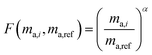
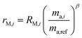
Fractionation laws are used to model mass dependent fractionation by relating the isotope amount ratios before a process has occurred to the isotope amount ratios after a process has occurred. In the case of instrumental mass bias, the process is the measurement itself. Mass fractionation laws follow this general form:where ri is the measured isotope amount ratio of the ith isotope to the reference isotope; Ri is the true ratio; F(ma,i,ma,ref) is a function that gives the magnitude of the change in the isotope amount ratio and is a function of the atomic masses of the ith and reference (denominator) isotopes, ma,i and ma,ref respectively.
There are several empirical fractionation laws which all follow this general form. They each use different functions to model mass dependent fractionation. The fractionation factor is defined differently in each model. For isotope ratio mass spectrometry, the most commonly applied fractionation model is called the exponential law:24
| |  | (2) |
where
α is the fractionation factor. This model is generally accepted as giving the best representation of the instrumental mass bias that occurs during ICP-MS measurements,
25 based on the comparison of predicted and measured isotopic fractionation.
2.2 Double-spike technique
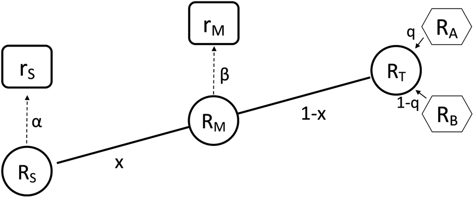
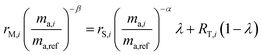
It is not possible to directly measure the absolute isotopic composition of a sample, as the measured isotopic compositions will be affected by some instrumental mass bias. The double-spike technique, originally published by Dodson in 1963 (ref. 26) and developed further by R.D. Russell in 1971,27 is used to correct for instrumental mass fractionation by mixing the sample being measured with a calibrated double-spike, also known as the tracer. The double-spike is composed of two single spikes which are materials that have been highly enriched (typically >95%) in a single isotope. The technique can only be applied to elements with at least four isotopes. Fig. 1 outlines the basic process of double-spiking.
 |
| | Fig. 1 This figure shows the mixture of the double-spike RT, which is made up of primary spikes RA and RB, with sample RS to form RM. The mixture consists of a proportion per mole x of the sample and (1 − x) of the double-spike. Measurements of the mixture and sample are fractionated with fractionation factors β and α respectively resulting in rM and rS. | |
The measured isotopic composition of the sample and sample-spike mixture is affected by instrumental mass bias represented by α and β for the sample and sample-spike mixture respectively. If the double-spike is calibrated, as described in Section 2.3, these fractionation factors can be determined.
The isotope amount ratios of the mixture are described by the following equation:28
| | | RM,i = RS,iλ + RT,i(1 − λ) | (3) |
where
RM,i,
RS,i and
RT,i are the
ith true isotope amount ratios of the mixture, sample and double-spike respectively, and
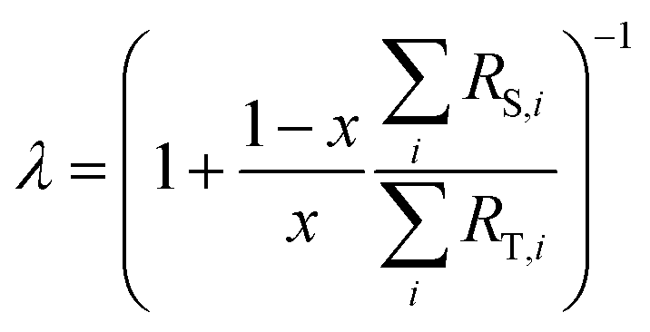
λ is related to the proportion by mole,
x, of the spike in the mixture as follows:
| | 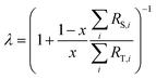 | (4) |
The sums are taken over all isotope amount ratios including the unitary ratio (i = ref). If the double-spike is assumed to be calibrated and the measurements of the unspiked sample and the sample-spike mixture are not calibrated, the resulting isotopic compositions which are fractionated from their true values due to instrumental mass bias are:
| |  | (5) |
| |  | (6) |
Rearranging and combining eqn (3), (5) and (6) we are left with the equation:
| |  | (7) |
This equation has three unknowns: α, β and λ. By using three different isotope amount ratios, we have three equations with three unknowns. Although this system of equations cannot be solved analytically, it can be determined using numerical techniques, such as the FindRoot command built into Wolfram Mathematica. Once the system is solved, α is applied to eqn (5) to determine the true isotopic composition of the sample. Eqn (4) can also be used to determine the proportion of spike in the mixture, which can then be applied to determine the amount of molybdenum in the sample if it is unknown.
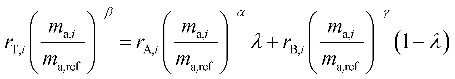
2.3 Double-spike calibration
In order for the double-spike method to be used to determine an absolute isotopic composition, the isotopic composition of the double-spike must be properly calibrated such that the instrumental mass bias has been corrected. The double-spike mixture is defined similarly to eqn (7), except that no ratios are calibrated:| | 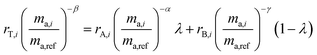 | (8) |
where rA,i and rB,i are the ith isotope amount ratios of each of the primary spikes, and λ is defined as:| | 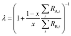 | (9) |
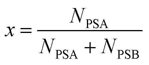
where x is the mole fraction of spike PSA in the mixture. x is related to the number of moles of each primary spike used:| | 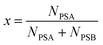 | (10) |
The amount of each spike added to the mixture is measured gravimetrically. The number of moles of each primary spike added is related to the mass (g) of the primary spike by:
| | 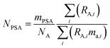 | (11) |
where
mPSA is the mass (g) of the spike used,
ma,i is the atomic mass (Da) of the
ith isotope, and
NA is the Avogadro constant.
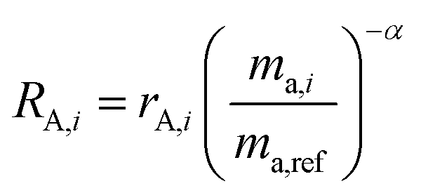
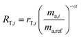
RA,i is related to
rA,i by:
| | 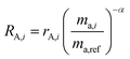 | (12) |
and similarly for
RB,i.
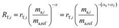
By measuring the mass of each primary spike in each double-spike mixture, we control the variable x and therefore λ. However, eqn (8) is still left with three unknowns: α, β and γ. These fractionation factors will be different as the instrumental mass bias changes over time between measurements of samples. However, by monitoring the change in mass bias over time, it is possible to determine the difference between the fractionation factors α, β and γ. This difference is then applied to correct the isotope amount ratios to have the same fractionation factors, α = β = γ. This is done using standard-sample bracketing which is described in the next section.
We are now left with a single equation with just one unknown, α. By using the isotope amount ratio of PSA's enriched isotope to PSB's enriched isotope for rA,i, rB,i and rT,i, eqn (8) can be solved numerically. For example, in this experiment 92Mo and 98Mo spikes are used, so the 98Mo/92Mo isotope amount ratios are needed for each of the single spikes and the double-spike mixture. This yields α and enables determination of the absolute composition of the double-spike:
| |  | (13) |
2.4 Standard-sample bracketing
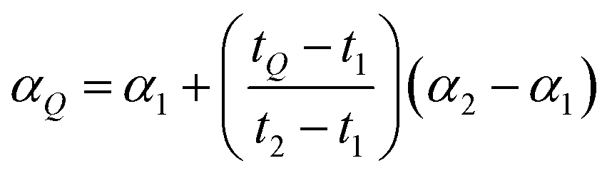
As described in the previous section, it is necessary to monitor the change in instrumental mass bias during each separate measurement to calibrate the double-spike isotopic composition. The mass bias of the instrument can change from day-to-day, and during a measurement session. This drift can be quantified by measuring a laboratory reference material, and comparing the measured ratios to an earlier measurement of the same material. A comparison of the results quantifies the change in mass bias that has occurred since the earlier measurement. Standard-sample bracketing is done by measuring a laboratory standard before and after the measurement of each sample enabling prediction of the relative instrumental fractionation during the measurement of the sample. An arbitrary starting value can be determined from any measurement of the standard, and is used to set a common reference point. Correcting for the mass bias drift to this reference point results in all instrumental fractionation factors being equal, though not equal to zero. Let rS0,i be the set of measured isotope amount ratios of our arbitrary starting value for the standard, while rS1,i and rS2,i are the measured isotope amount ratios of the standard measured before and after the measurement of the sample isotope amount ratios, which we will call rQ,i. The two bracketing standard measurements will be fractionated relative to the starting value with fractionation factors α1 and α2. Eqn (5) is solved for the average α:| | 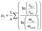 | (14) |
where n is the number of isotopes for the element, and similarly for α2. The fractionation factor of the sample, αQ, can then be determined reliably provided the fractionation drifts linearly in time between the bracketing standards (this assumption has been tested to be accurate to within ∼0.08‰):| | 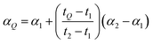 | (15) |
where t1, t2 and tQ are the times at which each measurement was taken. This brings each sample measurement back to the same relative fractionation as the arbitrary starting value.
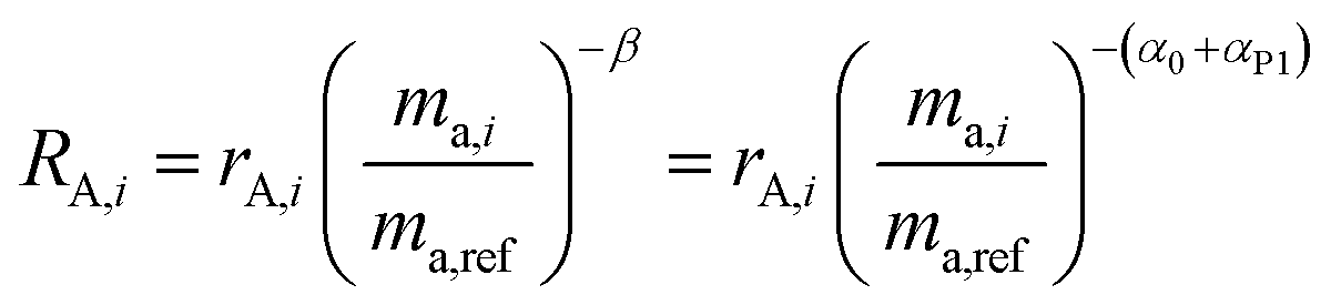
To demonstrate this, we suppose that the double-spike and a primary spike are measured at different times. Each would have a different instrumental fractionation factor, α and β:
| |  | (16) |
| |  | (17) |
By correcting for the relative fractionations αT and αP1, we are left with two measurements with the same fractionation factor, α0.
2.5 Blank subtraction
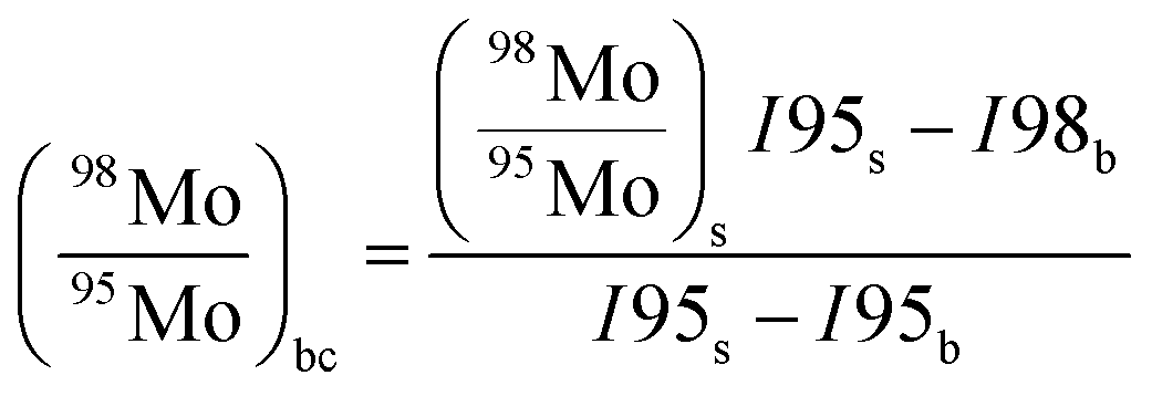
In order to correct for small interferences from residual molybdenum and other interferences in the instrument, a background correction was necessary. Prior to each measurement of a sample, the ion current intensities of freshly prepared 3% HNO3 were measured. This is called the blank. The measured ion current intensities from the blank were subtracted from the measured isotope abundance ratios of the sample using the following equation with an example of 98Mo/95Mo:| | 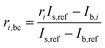 | (18) |
| | 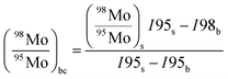 | (19) |
where ri,bc is the background corrected ratio, ri is the measured ratio for the sample, IS,ref and Ib,ref are the intensities of the reference isotope measured for the sample and blank respectively, and Ib,i is the intensity of the ith isotope of the blank.
2.6 Uncertainty propagation
Uncertainty propagation is done using Monte Carlo simulation by randomly choosing values from a normal distribution centered about each input value with a standard deviation equal to the uncertainty of the input value. This is done for all of the input values, and the uncertainties are determined after a sufficient number of iterations such that the results converge (n = 1000). This technique ensures that all sources of uncertainty are fully accounted for.
3 Measurement
3.1 Preparation of primary spikes
The 92Mo and 98Mo primary spikes, labeled PSA and PSB respectively, were prepared from Oak Ridge National Laboratory (ORNL) molybdenum metals individually enriched in 92Mo (Series ND, Batch 159390) and 98Mo (Series LB, Batch 134590). The metal powder spikes were each transferred into separate PFA containers and dissolved in 2 mL of concentrated Seastar Baseline HCl and 1 mL of concentrated Seastar Baseline HNO3. The solutions were then diluted to the required concentrations with 3% HNO3 prepared from Seastar Baseline concentrated HNO3 and pure water obtained from a MilliQ water purification system (18.2 MΩ cm). All masses were each measured 10 consecutive times using a Mettler-Toledo AT201 milligram balance. The means and standard deviations of these masses are reported in Table 1 along with the molybdenum concentrations of each primary spike.
Table 1 Masses measured during preparation of primary spikes (PSA (92Mo) and PSB (98Mo)), along with their Mo concentrations. Uncertainties at 1 s.d. based on ten replicate measurements
| Sample |
PSA |
PSB |
| Purity (%) |
99.99 ± 0.01 |
99.99 ± 0.01 |
| Weight of spike (g) |
0.14213(5) |
0.19276(9) |
| Weight of solution (g) |
117.7033(4) |
119.8722(15) |
| [Mo] (mg g−1) |
1.2075(4) |
1.6080(8) |
3.2 Preparation of double-spikes
In order to calibrate the isotopic composition of the double-spikes, a set of mixtures were made containing different proportions of primary spikes A (92Mo) and B (98Mo). Eight different mixtures were prepared in order to improve the accuracy and relative uncertainty of the calibration. An individual mixture may be subject to offsets during the mass measurements. By preparing eight different mixtures, the random error can be assessed and by varying the proportions of each spike in the mixtures, it is possible to choose the double-spike with the optimum ratio of PSA to PSB which is discussed later. The eight mixtures were prepared by pipetting the desired amount of each primary spike (PSA and PSB) into clean Teflon containers. The determined mass of each spike in each mixture is reported in Table 2.
Table 2 Masses of each primary spike used in each mixture. Amounts were chosen to include PSA to PSB molybdenum mass ratios approximately between 5![[thin space (1/6-em)]](https://www.rsc.org/images/entities/char_2009.gif) :1 and 1:5. Uncertainties at 1 s.d. based on ten replicate measurements
:1 and 1:5. Uncertainties at 1 s.d. based on ten replicate measurements
| Mixture |
MassPSA (g) |
MassPSB (g) |
| ABI-1 |
13.018(5) |
12.415(3) |
| ABI-2 |
12.667(6) |
6.330(4) |
| ABI-3 |
12.556(9) |
3.100(3) |
| ABI-4 |
12.464(10) |
1.646(3) |
| ABII-1 |
9.730(3) |
6.021(3) |
| ABII-2 |
6.704(3) |
6.055(3) |
| ABII-3 |
2.999(3) |
6.011(3) |
| ABII-4 |
1.512(3) |
6.015(3) |
3.3 MC-ICP-MS operation
All isotopic composition measurements were taken using a Thermo Scientific Neptune MC-ICP-MS. Multiple samples were measured in succession automatically using the Elemental Scientific auto-sampler. The sample was introduced to the plasma through a Glass Expansion nebulizer (100 μL min−1) and cyclonic spray chamber (20 mL). The excess liquid was removed from the spray chamber with a peristaltic pump. Table 3 outlines the operating conditions of the plasma. The sample and auxiliary gas flow, the torch position, and the focus settings were optimized to ensure maximum intensity, good peak shape, and good stability.
Table 3 MC-ICP-MS operating parameters
| Parameter |
Setting |
| RF power |
1200 W |
| Cool gas flow |
16 L min−1 |
| Aux gas flow |
∼1 L min−1 |
| Sample gas |
∼1 L min−1 |
| Sample uptake rate |
100 μL min−1 |
Eight Faraday cups were used to collect the seven isotopes of molybdenum along with 91Zr+ simultaneously. This allowed for the constant measurement of 91Zr+ to monitor possible isobaric interferences on 92Mo+, 94Mo+ and 96Mo+. 91Zr+ was collected on cup L4 with a 1012 Ω resistor, while the molybdenum isotopes were collected on cups L3–H3 each with 1011 Ω resistors. Amplifier gain calibration was performed regularly.
A typical measurement session began by allowing the instrument to warm up for a minimum of one hour while aspirating 3% HNO3. The laboratory tuning standard, PlasmaCal Molybdenum solution, was then used to tune the instrument. This included optimization of the operating parameters and focus settings for good peak shape, stability and intensity, as well as collection of a set of Mo isotope amount ratios. The intensity of 98Mo+ was at least 2 V, and the normalized isotope amount ratios had an internal precision typically less than 25 ppm. Measurement blanks were always monitored by measuring freshly prepared 3% HNO3 by collecting a set of ratios using the same method as used for samples. The concentration of molybdenum in all samples was approximately 200 ppb up to 2000 ppb in special cases discussed below.
The method used for each measurement was as follows. First a peak centering was performed on mass 98Mo, followed by a measurement of the electronic baseline by defocussing the ion beam. Next, seven blocks of 10–20 measurement cycles were performed. Each cycle measured the intensity at each cup with an integration time of 8.134 s. These intensities were converted to isotope amount ratios in the Data Evaluation software from the Neptune Multicollector software version 3.2.
A typical automated sequence included several measurements of NIST SRM 3134 Mo solution for standard-sample bracketing. After each measurement, a minimum 60 s wash was performed with 3% HNO3 to remove the residual molybdenum from the nebulizer and spray chamber, followed by a measurement of the background in clean 3% HNO3. Offline data analysis included mass bias drift correction and background correction as described in subsections 2.4 and 2.5.
3.4 Uncalibrated measurement of NIST SRM 3134
The internal standard used in the laboratory is NIST SRM 3134 Molybdenum Standard Solution, Lot # 891307 with a stock concentration of 9.99 mg g−1. This is an internationally available standard reference material. The first step is to establish an unnormalized isotopic composition to be used as a common reference value for standard sample bracketing. Table 4 shows the results of six consecutive isotopic composition measurements of the SRM 3134 standard. The internal precision for all measurements is ∼10 ppm (1 s.d.) and is not higher than 20 ppm.
Table 4 Unnormalized results with background correction for six consecutive measurements of SRM 3134
| Run # |
95 (V) |
92/95 |
94/95 |
96/95 |
97/95 |
98/95 |
100/95 |
| 1 |
1.51 |
0.877142 |
0.569148 |
1.067993 |
0.623938 |
1.607856 |
0.665910 |
| 2 |
1.53 |
0.877135 |
0.569151 |
1.067993 |
0.623935 |
1.607863 |
0.665901 |
| 3 |
1.53 |
0.877009 |
0.569131 |
1.068026 |
0.623978 |
1.608047 |
0.666049 |
| 4 |
1.59 |
0.876301 |
0.568998 |
1.068279 |
0.624299 |
1.608970 |
0.666831 |
| 5 |
1.52 |
0.876169 |
0.568977 |
1.068337 |
0.624345 |
1.609182 |
0.666939 |
| 6 |
1.58 |
0.876228 |
0.569078 |
1.068357 |
0.624352 |
1.609278 |
0.666938 |
The ratios varied substantially over the course of the measurement set as the mass bias of the mass spectrometer drifted. To correct for the drift in mass bias over the course of a measurement session, it is common to normalize the ratios by performing a mass bias correction based on the single isotope amount ratio. However, this necessarily eliminates the uncertainty in that ratio, and transfers it to the other ratios. All ratios are fluctuating, so it is important to preserve the uncertainty in each isotope amount ratio measurement and not transfer a single ratio's uncertainty to the others. This was done by calculating the fractionation factor α for each measured isotope amount ratio compared to the first run and taking the average α of all six ratios:
| | 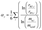 | (20) |
where
αj is the average fractionation factor of the
jth run,
rRJ,i and
rR1,i are the
ith measured ratios of the
jth run and first run respectively, and
ma,i and
ma,ref are the atomic masses of the
ith and reference isotopes respectively. This average
α is then used to correct for the internal mass bias drift:
| | 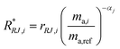 | (21) |
where
R*RJ,i is the
ith internal mass bias corrected ratio for run
j.
Table 5 shows the internally normalized ratios for the six measurements of SRM 3134. After correcting for the mass bias drift, the external precision for each isotope amount ratio was determined for this measurement session to be 20–70 ppm. The average isotope amount ratios were used as the common reference value for standard-sample bracketing for all further measurements.
Table 5 Mass bias drift corrected isotope amount ratios for six consecutive measurements of SRM 3134. Uncertainties are reported at 1 s.d.
| Run # |
92/95 |
94/95 |
96/95 |
97/95 |
98/95 |
100/95 |
| 1 |
0.877142 |
0.569148 |
1.067993 |
0.623938 |
1.607856 |
0.665910 |
| 2 |
0.877133 |
0.569150 |
1.067994 |
0.623936 |
1.607867 |
0.665904 |
| 3 |
0.877110 |
0.569153 |
1.067986 |
0.623932 |
1.607867 |
0.665927 |
| 4 |
0.877039 |
0.569156 |
1.067986 |
0.623958 |
1.607658 |
0.665934 |
| 5 |
0.877021 |
0.569160 |
1.067999 |
0.623951 |
1.607667 |
0.665903 |
| 6 |
0.877011 |
0.569246 |
1.068046 |
0.623990 |
1.607885 |
0.665986 |
| Mean |
0.87708(6) |
0.56917(4) |
1.06800(2) |
0.62395(2) |
1.60780(10) |
0.66593(3) |
3.5 Measurement of primary spikes
Now that the unnormalized isotope amount ratios of the lab standard have been determined, it is possible to measure the isotopic composition of the rest of the calibration materials beginning with each of the primary spikes. The primary spikes present a unique challenge as they are highly enriched in a single isotope. When the molybdenum concentration is 200 ppb, such that the spiked isotope is near the maximum measurable intensity (<50 V), the unspiked isotopes will have intensities that are 170–520 times smaller (as low as 50 mV). The baselines were greater than 0.1 mV, and the backgrounds were up to 0.5 mV amounting to up to 1% of the signal intensity. This problem was resolved by making two separate sets of measurements for each spike. The first was measurement of the spike with a normal concentration (∼200 ppb), while the second was measurement of the spike with a much higher concentration spike (2000 ppb). During the second measurement, the spiked isotope's ion beam could damage the Faraday cup and amplifiers, so the Faraday cup was moved to not collect the spiked isotope. This allowed for a precise determination of the major and minor isotope amount ratios.
Table 6 shows the measured ratios of the 92Mo spike, primary spike A (PSA), and the 98Mo spike, primary spike B (PSB). The results from the high concentration measurements were used for the low abundance isotopes, while the results from low concentration measurements were used for the enriched isotope.
Table 6 Mass bias drift corrected isotope amount ratios for PSA and PSB. Each measurement was repeated 4 times. The first run is normalized using standard-sample bracketing. The consecutive runs are normalized to the first run similarly to what was done for the lab standard. Uncertainty at 1 s.d.
| Spike |
92/95 |
94/95 |
96/95 |
97/95 |
98/95 |
100/95 |
|
| PSA Lo |
171.640(10) |
1.29255(7) |
0.69234(4) |
0.34620(7) |
0.8507(4) |
0.6042(2) |
|
| PSA Hi |
— |
1.29242(7) |
0.692285(17) |
0.34621(2) |
0.85009(5) |
0.60452(3) |
|
| PSB Lo |
0.566(7) |
0.45876(8) |
1.6475(3) |
2.8289(10) |
523.79(18) |
1.6011(5) |
|
| PSB Hi |
0.57325(7) |
0.45891(3) |
1.64583(4) |
2.82422(19) |
— |
1.5980(2) |
|
3.6 Measurement of double-spikes
The isotopic compositions of the double-spikes were measured and the mass bias drift was corrected using standard-sample bracketing. The n(98Mo)/n(92Mo) isotope amount ratios were required for the calibration of the double-spikes, while the remaining ratios were necessary when applying the double-spike technique to measure the isotopic composition of samples. Table 7 contains the measured ratios for each of the mixtures.
Table 7 Isotope amount ratios for spike mixtures. Results are normalized using standard-sample bracketing. Uncertainties are the range of two replicate analyses
| Spike mixture |
92/95 |
94/95 |
96/95 |
97/95 |
98/95 |
100/95 |
98/92 |
| ABI-1 |
119.620(11) |
1.03908(18) |
0.98250(12) |
1.10064(8) |
159.741(2) |
0.90680(17) |
1.33541(11) |
| ABI-2 |
139.79(8) |
1.1373(2) |
0.87009(9) |
0.80844(8) |
98.21(3) |
0.78969(4) |
0.70256(16) |
| ABI-3 |
154.2849(10) |
1.20781(11) |
0.78912(18) |
0.59814(11) |
53.952(7) |
0.7053(3) |
0.34969(4) |
| ABI-4 |
161.93(13) |
1.2453(5) |
0.7466(4) |
0.48772(12) |
30.689(19) |
0.6611(2) |
0.18951(3) |
| ABII-1 |
133.80(3) |
1.1081(3) |
0.903223(12) |
0.89433(3) |
116.296(7) |
0.82407(4) |
0.86915(12) |
| ABII-2 |
121.49(2) |
1.0482(3) |
0.97223(15) |
1.0737(3) |
154.09(3) |
0.89602(4) |
1.26839(4) |
| ABII-3 |
89.6853(7) |
0.8933(3) |
1.14937(2) |
1.5338(2) |
250.989(14) |
1.08056(8) |
2.79855(14) |
| ABII-4 |
61.192(10) |
0.75409(16) |
1.3086(3) |
1.94720(11) |
338.04(9) |
1.2465(3) |
5.5242(6) |
3.7 Overall fractionation correction
The uncalibrated isotopic compositions of the primary spikes and double-spikes have been measured and it was then possible to determine the true isotopic composition of the double-spikes. The method described in Section 2.3 was implemented in Mathematica, and the results follow in Table 8.
Table 8 List of calculated α's for each of the double-spike mixtures. The uncertainty was determined by Monte Carlo simulation with N = 1000 iterations. Uncertainties at 1 s.d.
| Spike |
α
|
| ABI 1 |
1.579(12) |
| ABI 2 |
1.577(17) |
| ABI 3 |
1.57(2) |
| ABI 4 |
1.59(4) |
| ABII 1 |
1.590(14) |
| ABII 2 |
1.620(16) |
| ABII 3 |
1.59(2) |
| ABII 4 |
1.57(4) |
| Mean |
1.59(3) |
The mean value for α calculated was applied to the double-spike isotope amount ratios to determine their absolute isotopic compositions. ABI-2 was chosen as having the optimum proportion of 92Mo and 98Mo primary spikes based on the Rudge “Double-spike toolbox”,28 which gives a list of the optimal double-spikes depending on the isotopes used, based on the lowest predicted uncertainty. The absolute isotope amount ratios of ABI-2 are reported in Table 9.
Table 9 Absolute isotope amount ratios for ABI2, calculated using mean α from Table 8. The uncertainty propagated from the isotope amount ratio measurement uncertainty and the uncertainty in α using Monte Carlo simulation. Uncertainty at 1 s.d.
| Sample |
92/95 |
94/95 |
96/95 |
97/95 |
98/95 |
100/95 |
| ABI2 |
147.09(13) |
1.1566(3) |
0.8558(2) |
0.7821(3) |
93.49(7) |
0.7279(8) |
3.8 Instrumental fractionation correction for SRM 3134
The calibrated isotopic composition of the double-spike can now be used to determine the absolute isotopic composition of the reference materials. As described in Section 2.2, eqn (7) is used to determine α, the fractionation factor, by solving for α, β, and λ. The value of α can then be used to correct for the instrumental mass bias during the measurement of the sample's isotopic composition.
Two of the three required sets of ratios have already been determined in the previous sections: the calibrated isotope amount ratios for the double-spike and the uncalibrated isotope amount ratios for our lab standard, which were measured and used for standard-sample bracketing. The third set of ratios requires measurement of a mixture of the standard and double-spike.
When preparing the mixture of sample and double-spike, it was important to control the ratio of double-spike to sample. If there was too much double-spike, the unspiked isotopes would be difficult to measure, increasing the uncertainty. If there was too little double-spike, the spiked isotopes would be difficult to differentiate from the sample, also increasing the uncertainty. The optimal relative amount of double-spike is between 40% and 60%.
The calculation of α requires three isotope amount ratios, two of which must include the two spiked isotopes (i.e. n(92Mo)/n(95Mo) and n(98Mo)/n(95Mo)), while the third can be chosen from the remaining ratios. When choosing the third ratio, it is important to select one that is free from interferences. For this reason, the n(94Mo)/n(95Mo) and n(96Mo)/n(95Mo) ratio was not used, since there can be a 94Zr+ interference and an unidentified mass-96 interference of up to 0.5 mV has been observed. The best precision was obtained using n(97Mo)/n(95Mo) as the third ratio, so it was used for all calculated results. The value of α determined was α = 1.5847(10). For comparison, the α values determined by using the other isotopes as the third ratio are presented in Table 10. It is clear that the choice of the third ratio does not impact the final result more than the uncertainty. This validates the use of the blank subtraction for the background correction, especially for 96Mo+ which cannot be corrected otherwise.
Table 10 List of calculated α's using each third isotope amount ratio. The best precision is obtained using n(97Mo)/n(95Mo) as the third ratio, although all four results are within the uncertainty of each other. Uncertainties at 1 s.d.
| Third ratio |
α
|
|
n(94Mo)/n(95Mo) |
1.5849(36) |
|
n(96Mo)/n(95Mo) |
1.5837(14) |
|
n(97Mo)/n(95Mo) |
1.5847(10) |
|
n(100Mo)/n(95Mo) |
1.5850(13) |
3.9 Absolute isotopic composition and atomic weight of the SRM 3134 molybdenum standard
The absolute isotopic composition of the SRM 3134 molybdenum reference material was determined by applying the correction factor α, obtained above. The uncertainty in the value of α for the standard was expanded to include the uncertainty of the value of α found in the calibration of the double-spike, α = 1.59(3). This propagated uncertainty dominates the uncertainty in the α used for the correction of the standard, and was propagated by Monte Carlo simulation: α-97 = 1.58(3). The absolute isotopic composition is determined from the isotope amount ratios using the following equation:| |  | (22) |
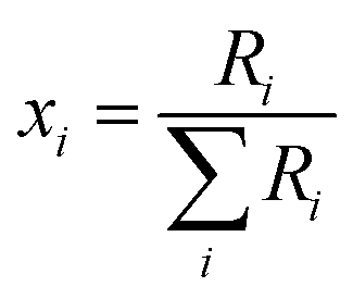
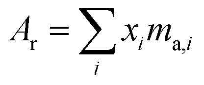
where the sum is over all ratios including the unitary ratio. The atomic weight is determined from the absolute isotopic composition as follows:| |  | (23) |
where ma,i is the atomic mass of the ith isotope.
By applying the correction factor α to the unnormalized isotope amount ratios obtained in Section 3.8, the absolute isotopic composition and atomic weight of the SRM 3134 molybdenum standard were determined. Table 11 shows the corrected isotope amount ratios for SRM 3134, along with the absolute isotopic composition and atomic weight.
Table 11 The isotope amount ratios, absolute isotopic composition and atomic weight of molybdenum in SRM 3134. All uncertainties are at 2 s.d. and are propagated from the uncertainties in the measured isotope amount ratios and the uncertainty in the fractionation correction factor by Monte Carlo simulation. For comparison, the previous measured isotopic composition and atomic weight by Wieser and De Laeter2 are reported with the uncertainty increased to 2 s.d., along with the IUPAC representative isotopic composition derived from the Wieser and De Laeter results with the expanded uncertainty29
| Isotope |
Isotope amount ratio (XMo/95Mo) |
Isotopic composition (%) |
Previous best measured composition2 |
Representative composition (IUPAC)29 |
| 92 |
0.9229(16) |
14.65(4) |
14.525(3) |
14.53(30) |
| 94 |
0.5788(4) |
9.187(12) |
9.151(15) |
9.15(9) |
| 95 |
1(0) |
15.873(10) |
15.838(20) |
15.84(11) |
| 96 |
1.0504(6) |
16.673(3) |
16.67(4) |
16.67(15) |
| 97 |
0.6037(8) |
9.582(6) |
9.599(15) |
9.60(14) |
| 98 |
1.530(3) |
24.29(3) |
24.39(4) |
24.39(37) |
| 100 |
0.6139(18) |
9.74(2) |
9.82(10) |
9.82(31) |
|
|
|
|
|
|
| Atomic weight: 95.949(3) |
95.960(5) |
95.96(2) |
The determined atomic weight of Ar = 95.949(3) is lower than the last reported value of Ar = 95.96(2), though within the IUPAC expanded uncertainty.29 The Wieser and De Laeter measurement was performed using TIMS and a correction to the instrumental mass bias was applied using a double-spike technique. Prior to the mass bias correction, the raw data gave an atomic weight of Ar = 95.94, which is equal to the earlier IUPAC values determined by TIMS. With TIMS, each measurement is performed with a separate filament and it is not possible to control the fractionation from filament to filament using a technique like standard-sample bracketing. Therefore, the relative instrumental fractionation in the measurements of the isotopic composition of the spikes could not have been monitored and fully corrected. Wieser and De Laeter used the average of 11 measurements of their molybdenum reference material as their unnormalized isotopic composition. A comparison of these 11 measurements shows a range of internal fractionation of up to ±2‰ per Da, corresponding to an uncertainty in the fractionation exponent α of ±0.2 at 2 s.d. If the uncertainty in the fractionation correction factor is increased to ±0.2, the final uncertainty in the atomic weight becomes Ar = 95.96(2) (2 s.d.), matching the IUPAC expanded uncertainty. It is likely that the isotopic composition of the spike materials that was measured led to a determined fractionation factor that was larger than the average fractionation factor for the molybdenum reference material.
The uncertainty reported in this paper is an order of magnitude less than that of the currently published IUPAC value, and the atomic weight is closer to the historic value of Ar = 95.94(2).1
3.10 Relative composition of other pure molybdenum reference materials
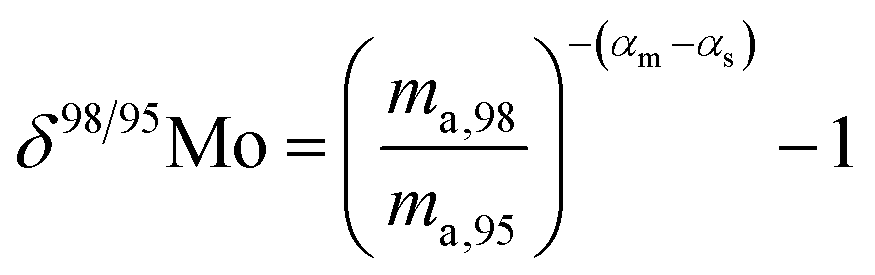
When measuring natural or synthetic samples, the absolute isotopic composition is typically not reported. Instead the isotopic composition is compared with that of a laboratory standard, and the results are reported as a delta (δ) value in permille.30 For molybdenum, it is most common to report δ98/95Mo values, calculated as follows:| | 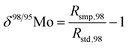 | (24) |
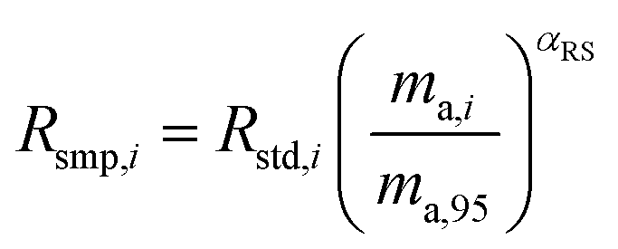
where δ98/95Mo is the delta value in permille, Rsmp,98 is the absolute 98Mo/95Mo ratio of the sample, free of any instrumental mass bias, and Rstd,98 is the absolute 98Mo/95Mo isotope amount ratio of the standard. The sample is usually assumed to have undergone mass-dependent fractionation relative to the standard. This allows the isotopic composition of the sample to be equal to the isotopic composition of the standard with an added fractionation factor:| | 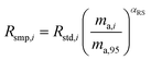 | (25) |
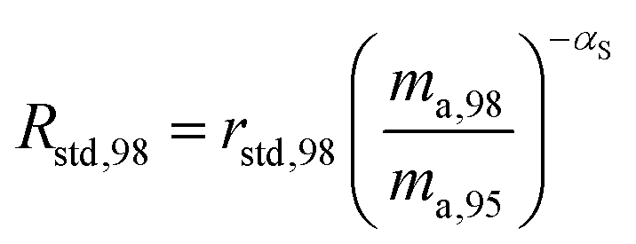
where αRS is the relative fractionation factor of the sample to the standard, and ma,i and ma,95 are the atomic masses of iMo and 95Mo. If the sample has undergone mass independent fractionation, such that the above equation does not hold true, a separate measurement of the isotopic composition prior to the sample being mixed with the spike is necessary, but this special case will not be discussed further since the selected samples have only undergone mass-dependent fractionation. The absolute isotope amount ratios of the standard and sample can be related to measurement of the standard as follows:| | 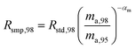 | (26) |
| | 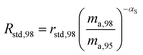 | (27) |
where rstd,98 is the isotope amount ratio of the standard. αm is determined in the same manner as αs was determined in Section 3.8 by preparing a mixture of the sample and double spike. If eqn (26) and (27) are substituted into eqn (24), we obtain the following:| | 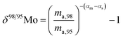 | (28) |
The difference of the values of α determined for the sample and standard is sufficient to calculate the delta value.
Mixtures were prepared with two widely available pure molybdenum reference materials including SCP Science PlasmaCAL Standard - Molybdenum, Lot # SC9306057, and a solution of molybdenum that was prepared by dissolving a 99.993% spectroscopically pure metal rod (Johnson-Matthey Chemicals Ltd., JMC 726, No. S-8555). The latter was prepared at Curtin University, Western Australia, and was used in the most recent determination of the absolute isotopic composition of molybdenum.2Table 12 shows the determined delta values for these two reference materials as compared to the calibrated SRM 3134 measurement. Each of the samples had a relatively small negative fractionation compared to the SRM 3134 reference material. These fractionations could have been caused by the different chemical and physical processes used in the purification of the molybdenum, or by having different sources of molybdenum for the manufacturing of the standard material.
Table 12 Delta values determined for three synthetic molybdenum samples. Uncertainties calculated from three replicate measurements of each sample at 2 s.d.
| Sample |
δ
98/95Mo (‰) |
| Curtin-Mo |
−0.45(12) |
| PlasmaCal |
−0.42(10) |
The natural variation of the isotopic composition of molybdenum has a δ98/95Mo of −1.5‰ to +3‰,31 relative to the Rochester JMC standard. This standard has a similar composition to the JMC Bern standard,31 which has been measured relative to SRM 3134 by Greber et al.22 to have a δ98/95Mo = −0.25(8)‰. Applying this range, corrected to be relative to SRM 3134, the atomic weight calculation gives a range of the atomic weights of molybdenum in natural samples of 95.944 to 95.956, including the uncertainty in the atomic weight of SRM 3134. This range is twice as large as the uncertainty of the atomic weight of SRM 3134 but is less than the uncertainty of the published IUPAC value. Based on these data the atomic weight of molybdenum in natural samples is the interval Ar = [95.944, 95.956] with the best measurement of Ar = 95.9488(32) (2 s.d.).
Acknowledgements
The Isotope Laboratory in the Department of Physics and Astronomy at the University of Calgary is supported by funding through an NSERC Discovery Grant. The authors gratefully acknowledge Dr Robert Loss for the discussions and suggestions for calibration of the molybdenum double spike. The paper benefited greatly from the insightful comments of two anonymous reviewers.
References
- M. E. Wieser and M. Berglund, Pure Appl. Chem., 2009, 81, 2131–2156 CrossRef CAS.
- M. E. Wieser and J. R. De Laeter, Phys. Rev. C: Nucl. Phys., 2007, 75, 055802 CrossRef.
- G. P. Baxter, O. Hönigschmid and P. Lebeau, J. Chem. Soc., 1938, 1101–1109 RSC.
- A. E. Cameron and E. Wichers, J. Am. Chem. Soc., 1962, 84, 4175–4197 CrossRef CAS.
- IUPAC Commission on atomic weights, Pure Appl. Chem., 1970, 21, 91–108 CrossRef.
- IUPAC Commission on atomic weights, Pure Appl. Chem., 1976, 47, 75–95 CrossRef.
- V. Rama Murthy, Geochim. Cosmochim. Acta, 1963, 27, 1171–1178 CrossRef.
- L. J. Moore, L. A. Machlan, W. R. Shields and E. L. Garner, Anal. Chem., 1974, 46, 1082–1089 CrossRef CAS.
- N. E. Holden, R. L. Martin and I. L. Barnes, Pure Appl. Chem., 1983, 55, 1119–1136 CrossRef CAS.
- T. B. Coplen, J. K. Böhlke, P. De Bièvre, T. Ding, N. E. Holden, J. A. Hopple, H. R. Krouse, A. Lamberty, H. S. Peiser, K. Révész, S. E. Rieder, K. J. R. Rosman, E. Roth, P. D. P. Taylor, R. D. Vocke Jr and Y. K. Xiao, Pure Appl. Chem., 2002, 74, 1987–2017 CrossRef CAS.
- M. E. Wieser and J. R. De Laeter, Int. J. Mass Spectrom., 2000, 197, 253–261 CrossRef CAS.
- R. D. Loss, L. Schultz, J. K. Böhlke, T. Ding, M. Ebihara, G. Ramendik, P. D. P. Taylor, M. J. Berglund, C. A. M. Brenninkmeijer, H. Hidaka, D. J. Rokop, T. Walczyk and S. Yoneda, Pure Appl. Chem., 2003, 75, 1107–1122 CrossRef CAS.
- J. R. De Laeter, J. K. Böhlke, P. De Bièvre, H. Hidaka, H. S. Peiser, K. J. R. Rosman and P. D. P. Taylor, Pure Appl. Chem., 2003, 75, 683–800 CrossRef CAS.
- N. Dauphas, L. Reisberg and B. Marty, Anal. Chem., 2001, 73, 2613–2616 CrossRef CAS.
- N. Dauphas, B. Marty and L. Reisberg, Astrophys. J., 2002, 565, 640–644 CrossRef CAS PubMed.
- Q. Yin, S. B. Jacobsen and K. Yamashita, Nature, 2002, 415, 881–883 CrossRef CAS PubMed.
- M. E. Wieser, S. Barry and J. R. De Laeter, J. Radioanal. Nucl. Chem., 2012, 293, 949–954 CrossRef CAS PubMed.
- J. Barling, G. L. Arnold and A. D. Anbar, Earth Planet. Sci. Lett., 2001, 193, 447–457 CrossRef CAS.
- C. Siebert, T. F. Nägler, F. von Blanckenburg and J. D. Kramers, Earth Planet. Sci. Lett., 2003, 211, 159–171 CrossRef CAS.
- M. E. Wieser and J. R. De Laeter, Phys. Rev. C: Nucl. Phys., 2001, 64, 243081–243087 CrossRef.
- M. E. Wieser and J. R. De Laeter, Int. J. Mass Spectrom., 2009, 286, 98–103 CrossRef CAS PubMed.
- N. D. Greber, C. Siebert, T. F. Nägler and T. Pettke, Geostand. Geoanal. Res., 2012, 36, 291–300 CrossRef CAS.
- H. Wen, J. Carignan, C. Cloquet, X. Zhu and Y. Zhang, J. Anal. At. Spectrom., 2010, 25, 716–721 RSC.
- J. Meija, L. Yang, R. Sturgeon and Z. Mester, Anal. Chem., 2009, 81, 6774–6778 CrossRef CAS PubMed.
- L. Yang, Mass Spectrom. Rev., 2009, 28, 990–1011 CrossRef CAS PubMed.
- M. H. Dodson, J. Sci. Instrum., 1963, 40, 289–295 CrossRef.
- R. D. Russell, J. Geophys. Res., 1971, 76, 4949–4955 CrossRef.
- J. F. Rudge, B. C. Reynolds and B. Bourdon, Chem. Geol., 2009, 265, 420–431 CrossRef CAS PubMed.
- M. Berglund and M. E. Wieser, Pure Appl. Chem., 2011, 83, 397–410 CrossRef CAS.
- W. A. Brand and T. B. Coplen, Isot. Environ. Health Stud., 2012, 48, 393–409 CrossRef CAS PubMed.
-
A. D. Anbar, Molybdenum stable isotopes: Observations, interpretations and directions, 2004, vol. 55, pp. 429–454 Search PubMed.
|
| This journal is © The Royal Society of Chemistry 2014 |
Click here to see how this site uses Cookies. View our privacy policy here.