DOI:
10.1039/C4CP03465A
(Perspective)
Phys. Chem. Chem. Phys., 2014,
16, 24128-24164
Anomalous diffusion models and their properties: non-stationarity, non-ergodicity, and ageing at the centenary of single particle tracking
Received
4th August 2014
, Accepted 19th September 2014
First published on 22nd September 2014
Abstract
Modern microscopic techniques following the stochastic motion of labelled tracer particles have uncovered significant deviations from the laws of Brownian motion in a variety of animate and inanimate systems. Such anomalous diffusion can have different physical origins, which can be identified from careful data analysis. In particular, single particle tracking provides the entire trajectory of the traced particle, which allows one to evaluate different observables to quantify the dynamics of the system under observation. We here provide an extensive overview over different popular anomalous diffusion models and their properties. We pay special attention to their ergodic properties, highlighting the fact that in several of these models the long time averaged mean squared displacement shows a distinct disparity to the regular, ensemble averaged mean squared displacement. In these cases, data obtained from time averages cannot be interpreted by the standard theoretical results for the ensemble averages. Here we therefore provide a comparison of the main properties of the time averaged mean squared displacement and its statistical behaviour in terms of the scatter of the amplitudes between the time averages obtained from different trajectories. We especially demonstrate how anomalous dynamics may be identified for systems, which, on first sight, appear to be Brownian. Moreover, we discuss the ergodicity breaking parameters for the different anomalous stochastic processes and showcase the physical origins for the various behaviours. This Perspective is intended as a guidebook for both experimentalists and theorists working on systems, which exhibit anomalous diffusion.
 Ralf Metzler | Ralf Metzler studied physics at Ulm University, where he also received his doctorate. As a postdoc he worked at Tel Aviv University and MIT. After his first faculty appointment at NORDITA in Copenhagen he moved to the University of Ottawa as Canada Research Chair in Biological Physics. In 2007 he became a professor at Technical University of Munich, since 2011 he has been the chair of Theoretical Physics at Potsdam University. Ralf works on stochastic processes, non-equilibrium statistical physics, crowded soft matter systems, and biological physics of gene regulation. Ralf received the Amos de Shalit Minerva, Feodor Lynen Humboldt, and Emmy Noether DFG fellowships. He is currently also Finland Distinguished Professor at Tampere University of Technology. |
 Jae-Hyung Jeon | Jae-Hyung Jeon received his PhD from Pohang University of Technology and Science, Korea. He then moved for postdoctoral studies to the Technical University of Munich, Germany and later to Tampere University of Technology in Finland. At present he is an assistant professor of statistical physics at the Korea Institute for Advanced Study in Seoul. His research interests include diffusion and transport processes in living cells and complex fluids, stochastic theory of anomalous diffusion models, DNA and membrane biophysics, as well as polymer physics. |
 Andrey G. Cherstvy | Andrey G. Cherstvy received his PhD in theoretical biophysics from Düsseldorf University in 2002. After several PostDoc terms, he currently conducts an independent DFG-funded research at Potsdam University. Andrey Cherstvy published about 50 papers, with the main focus on theoretical and computational biophysics, statistical mechanics, DNA, proteins, polyelectrolytes, membranes, and viruses. Recently, he has also become active in the fields of anomalous stochastic processes, tracer diffusion in biological cells, and ergodicity breaking. |
 Eli Barkai | Eli Barkai graduated from Tel Aviv University and currently is a professor of physics at Bar-Ilan university in Israel. In his postdoc studies with Bob Silbey he developed the theory of single molecule spectroscopy, which is also the subject of the current manuscript. His main research is focused on statistical physics, in particular weak ergodicity breaking and infinite ergodic theory. He together with Ralf Metzler and Yossi Klafter contributed to the field of anomalous diffusion in the development of fractional kinetic equations. He received the Yeshiahu Horowitz Science of complexity fellowship, the Krill prize for excellence in scientific research selected by the Wolf foundation, the Michael Bruno memorial award funded by Yad Hanadiv, and the Friedrich Wilhem Bessel award selected by the Humboldt foundation. |
1 Introduction and historical perspective
It is possible that the movements to be discussed here are identical with the so-called “Brownian molecular motion”; however, the information available to me regarding the latter is so lacking in precision, that I can form no judgment in the matter. This statement is part of the introduction of Albert Einstein's first and seminal 1905 paper on the theory of diffusion.1 It refers to the observations reported by Robert Brown in 1828 of small granules (or Molecules, as I shall term them) of  th to
th to  th of an inch extracted from larger pollen grains. Brown found these particles evidently in motion.2 He made meticulously sure that the motion he observed was not the effect of living matter, and he even studied the motion of such molecules as of a bruised fragment of the Sphinx.2 In his second, 1906 paper Einstein then quotes the experimental proof by Gouy3 that indeed the motion perpetuated by Robert Brown is caused by the irregular thermal movements of the molecules of the liquid, and thus described by Einstein's theory.1 As remarked by Marian Smoluchowski in his equally seminal 1906 article,4 Einstein reinvigorated the interest in Brownian motion. Since then, the interest in the molecular phenomenon of diffusion is unbroken.
Considering the local concentration difference and the counteracting flux of microscopic particles with a typical mean free path, Einstein derived the diffusion equation†1
| |
 | (1) |
with the coefficient of diffusion
K1 for the probability density function (PDF)
P(
x,
t) to find the particle under observation at position
x at time
t. This equation is indeed equivalent to Fick's second law for the concentration of a chemical substance originally presented by Adolf Fick from a combination of the continuity equation and the constitutive equation (Fick's first law).
5 If the particle is released at the origin at time
t = 0 in an unbounded space, the solution of the diffusion
equation (1) is the normalised Gaussian PDF
| |
 | (2) |
Einstein remarks that this solution is
that of the fortuitous error, which was to be expected.
1 From the PDF (2) we immediately obtain the variance
| |
 | (3) |
the so-called mean squared displacement (MSD). From the dynamic equilibrium of suspended particles Einstein (and later independently Smoluchowski) derived the celebrated relation
| |
 | (4) |
between the diffusion coefficient, thermal energy
kBT, the mass
m of the observed particle, and the friction coefficient
η of unit 1 s
−1. In the second equality of
eqn (4) we replaced the Boltzmann constant
kB by the ratio of the gas constant
R, quite precisely known at the time, and Avogadro's number
NA.
Yet another derivation of Brownian motion with the MSD (3) was published in 1908 by Paul Langevin using the concept of a stochastic force. The Langevin equation combines Newton's second law with the white Gaussian noise ξ(t) of zero mean and autocorrelation function 〈ξ(t)ξ(t′)〉 = 2K1δ(t − t′).6,7 In its overdamped form relevant for the single particle tracking experiments we will refer to below, it reads6,7
| |
 | (5) |
The Langevin formalism represents a very intuitive physical picture for Brownian motion. From the Langevin
eqn (5) it is easy to get back to the MSD (3). Likely prompted by discussions with his friend Paul Langevin,
8 the fundamental Einstein–Smoluchowski relation
(4) led Jean Perrin at the Sorbonne in Paris to conduct the first extensive and systematic measurement of the diffusion of single microscopic particles to determine Avogadro's number
NA.
‡9
While Perrin was confined to short measured trajectories and the need to use ensemble averages over not perfectly identical particles, to the best of our knowledge it was Ivar Nordlund at the University of Uppsala in Northern Sweden, who in 1914 came up with the innovative idea to record the motion of individual sedimenting mercury droplets on a moving film plate,13 see Fig. 1. Nordlund managed to produce impressively long individual time series of the droplet position. From separate analysis of each single trajectory he determined the diffusion coefficients of the traced droplets. The mass of the droplets was deduced from the sedimentation speed using Stokes' formula.13 In the sense of the combination of single particle tracking with the time series analysis of single recorded trajectories first performed by Nordlund, we celebrate this year the centenary of modern single particle tracking.
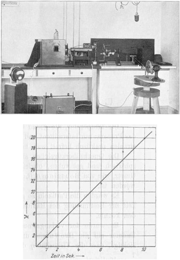 |
| | Fig. 1 Centennial single particle tracking experiments of Ivar Nordlund. Top: Nordlund's experimental setup with the light source, an infrared absorbing water-filled cylinder, and the clock-controlled, electromagnetic shutter (on the table to the left) constituting a stroboscope. Mounted on the separate optical table on the rack to the right, the object chamber with the mercury droplet, as well as the objective and the camera are the heart of the experiment: the camera is connected to an electric motor moving the photographic plate with constant velocity. Bottom: example for the time averaged mean squared displacement versus time (in seconds) from a single recorded mercury droplet. Images taken from ref. 13. | |
Nordlund's experimental setup, the MSD from a single trajectory, as well as a sample trajectory are shown in Fig. 1 and 2. Nordlund advocated in his paper that the principle of the method of measurement consists in the automated recording of the Brownian displacements of the particles in exactly identical time intervals, free of personal errors.13 Perrin's and Nordlund's studies prompted a string of diffusion experiments to determine the value of NA ever more precisely in the years to come, culminating in the high precision torsional diffusion experiments by Eugen Kappler, who in his PhD thesis at the University of Munich found the remarkable result NA = 60.59 × 10²² ± 1%.§14 We show the experimental shape of the torsional Brownian motion measured by Kappler in Fig. 3.
 |
| | Fig. 2 Example for the recorded motion of a ‘submicroscopic’ mercury droplet using the clock-driven stroboscope and a moving film plate in the setup shown in Fig. 1. The mass of the droplet could be determined from the droplet radius deduced from the sedimentation speed by use of Stokes' formula.13 Time is increasing from left to right. The stochastic, Brownian motion around the deterministic sedimentation with constant velocity can be clearly distinguished. Image taken from ref. 13. | |
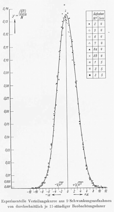 |
| | Fig. 3 Experimental verification of the Gaussian shape by Kappler14 with the original figure caption. The symbols represent nine different measurements of average duration of 11 hours of the torsional Brownian motion. | |
Hundred years after Nordlund's conception of single particle tracking by the analysis of individual particle traces, modern microscopic technology is routinely used by experimentalists to record the motion of fluorescently labelled single molecules or submicron tracer particles.¶15–18 In these experiments the recorded time series x(t′) is evaluated in terms of the time averaged MSD||
| |
 | (6) |
The time series
x(
t′) of length
t (the measurement time) is thus evaluated in terms of squared differences of the particle position separated by the so-called lag time
Δ which defines the width of the window slid along the time series
x(
t′). Typically,

is considered in the limit
Δ ≪
t to obtain good statistics. It is easy to show that for Brownian motion

as long as the measurement is sufficiently long. Compared with
eqn (3) we observe the equivalence
| |
 | (7) |
and therefore call the process
ergodic: ensemble averages and long-time averages are equivalent in the limit of long measurement times.
Apart from direct imaging of the motion of a tracer particle using a microscope, optical tweezer setups can be used to obtain an improved temporal and spatial resolution of a suitable tracer.20 Such single particle tracking can be used to measure the motion of tracers in quite complex media such as living biological cells.17,18 Alternatively to single particle tracking, which provides the time series x(t′) of the particle position, the diffusion of labelled molecules can be measured by methods such as fluorescence correlation spectroscopy (FCS),21 fluorescence recovery after photobleaching (FRAP),22 or fluorescence (Förster) resonant energy transfer (FRET).17,23 While these latter methods have many advantages—for instance, that they can measure the motion of smaller tracers—they have the intrinsic disadvantage that the quantity they measure is not the particle position but averages over the position such as the blinking correlation function of fluorescent particles entering and leaving the illuminated focal spot in FCS. Due to the underlying averaging, these latter methods thus do not provide the same full information as direct single particle tracking. We note that the MSD of stochastic systems may also be determined with techniques such as dynamic light scattering24 or laser Doppler velocimetry.25
Already in 1926 an exception to the linear time dependence (3) of the MSD of Brownian motion was analysed by Lewis Fry Richardson. For the relative diffusion of two tracer particles in a turbulent flow he observed strongly non-Brownian behaviour.26 He introduced the notion of non-Fickian diffusion and used a diffusion equation with separation dependent diffusivity  for the PDF q(l,t) of the relative displacement l to find the power-law MSD 〈l2(t)〉 ≃ t3 with the characteristic cubic scaling. Today anomalous diffusion typically refers to the power-law form**
of the MSD with the anomalous diffusion exponent
α and the generalised diffusion coefficient
Kα of physical dimension cm
2 (s
α)
−1. This is what we refer to in the following, distinguishing subdiffusion (0 <
α < 1) and superdiffusion (
α > 1).
The conditions assumed by Einstein in his derivation of the diffusion equation are (i) the independence of individual particles, (ii) the existence of a sufficiently small time scale beyond which individual displacements are statistically independent, and (iii) the property that the particle displacements during this time scale correspond to a typical mean free path distributed symmetrically in positive or negative directions. These assumptions, by the help of the central limit theorem, a forteriori lead to the Gaussian PDF (2) and thus to the diffusion equation (1). The model described by Einstein may therefore be viewed as a random walk or drunkard's walk, a concept introduced in the same year 1905 by Karl Pearson in his famed letter to Nature.30 The connection of the diffusion law to the random walk process was rendered more precisely by Smoluchowski.4
In anomalous diffusion processes, at least one of these fundamental assumptions is violated, and the strong convergence to the Gaussian according to the central limit theorem broken. In particular, by departing from one or more of the assumptions (i)–(iii), we find that there exist many different generalisations of the Einstein–Smoluchowski diffusion picture. Here we examine the properties of several popular and widely used anomalous diffusion models which are important for the evaluation and physical interpretation of single particle tracking data. These models are conceptually very different from each other, their only common ground being the non-Brownian form (8) of the MSD. We pay particular emphasis on their ergodic behaviour, that is, whether within the model the ensemble averaged MSD (8) has the same form as the time averaged MSD (6) or not, an important information for the evaluation of single particle tracking time series in terms of physical theories, which are usually formulated in terms of ensemble averages. We also check the ageing properties of the processes, that is, the potential dependence of physical observables such as the MSD on the time span between initialisation of the system and the start of the measurement. Both ergodicity breaking and ageing of a process are two sides of the same medal and are intimately connected to the (non-)stationarity properties.31,32
As we will see, numerous experiments using the above techniques demonstrate the non-Brownian diffusion of tracked biological cells as well as of tracer particles inside those very cells. Similarly, anomalous diffusion is often revealed for the motion of passive particles in complex liquids. One of the breakthroughs came with the study of Golding and Cox, who used single particle tracking of labelled messenger RNA (mRNA) molecules of some 100 nm in size in living bacteria cells to demonstrate that the motion of the molecule is subdiffusive,33 shown in Fig. 4. Even more interesting and thought-provoking was the fact that the time traces  of individual trajectories showed a massive scatter of amplitudes, similar to those shown in Fig. 8. The question whether this behaviour could be due to the intrinsic non-ergodicity of the anomalous diffusion performed by the mRNA molecules was in fact one of the ignition points for the research presented herein. We note that non-ergodicity in the sense discussed in the following is not restricted to the spatial diffusion of particles, but similar principles hold for certain processes revealing non-exponential dynamics, such as the blinking behaviour of individual quantum dots34 or laser cooling.35 To physically interpret such measurements we need to understand the time averages of individual time series. As we will see, this requires information beyond the conventional ensemble averages for a variety of anomalous diffusion processes.
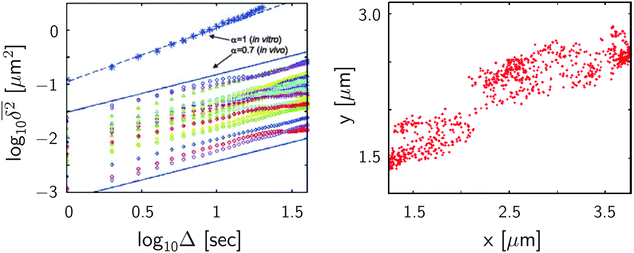 |
| | Fig. 4 Motion of labelled messenger RNA molecules in a living E. coli cell. Left: time averaged MSD of individual trajectories plotted as a function of the lag time Δ of eqn (6) shows pronounced trajectory-to-trajectory scatter. Yet all exhibit approximately the same anomalous diffusion exponent α ≈ 0.7, with some local variations. In contrast, the control experiment in water (stars) shows normal diffusion with α = 1. Right: points of the trajectory of an individual messenger RNA in the E. coli cell, showing that the molecule explores a major fraction of the bacterium's volume. (Adapted from ref. 33.) | |
2 A short navigation chart through this Perspective article
The main focus of this Perspective is two-fold. It is meant as an introduction to the theory of anomalous diffusion processes but also as a toolbox for the data analysis of anomalous stochastic dynamics. Consider the experimental results of single particle tracking experiments on fluorescently labelled messenger RNA molecules in a living E. coli bacteria cell shown in Fig. 4. Despite the fact that individual trajectories explore a large portion of the entire cell volume, the amplitude and the local slope of individual molecule traces, apart from the common subdiffusive trend, vary massively. Is this apparent irreproducibility an artefact or the result of the physical mechanism governing the molecule's motion? What is the exact physical origin of the variations in the slope? Will longer measurement times improve the statistics? Can we interpret the time averaged MSD shown here in terms of the ensemble results known for anomalous diffusion? Such questions will be pursued in what follows.
More concretely, this Perspective summarises a large variety of stochastic processes yielding anomalous diffusion of the power-law form 〈x2(t)〉 ≃ Kαtα. We mostly focus on subdiffusion with 0 < α < 1 but also consider superdiffusion characterised by α > 1 as well as ultraslow diffusion with a logarithmic form of 〈x2(t)〉. The fact that we consider this large range of anomalous diffusion processes is the non-universal nature of anomalous diffusion itself. Once we leave the realm of Brownian motion, we lose the confines of the central limit theorem forcing the processes to converge to the Gaussian behaviour predicted by Einstein. For this reason we address the most common processes effecting anomalous diffusion and compare their basic properties. The latter are important for the second purpose of this Perspective, namely, to provide a toolbox for the analysis of anomalous stochastic time series x(t). Quite commonly such analyses of time series from experiment or simulations are performed in terms of time averaged observables, in particular, the time averaged MSD  . We point out that the physical interpretation of the obtained behaviour of such time averages in terms of the typically available ensemble approaches may be treacherous: many of the anomalous diffusion processes discussed herein lead to a disparity between the ensemble and the time averaged observable, for instance, between the ensemble and time averaged MSDs
| |
 | (9) |
even in the limit of long measurement times. Moreover, it turns out that individual results for time averages such as

appear to be irreproducible, despite long measurement times. Such
strange kinetics32 was in fact observed in a number of experiments mentioned below. Instead of insufficient statistics, we show that such
weakly non-ergodic behaviour reflects the physical nature of the exact mechanisms effecting the observed stochastic dynamics.
The degree of the disparity between time and ensemble averaged observables and their apparent irreproducibility differ between the anomalous diffusion processes discussed hereafter. For each time series it is important to identify the exact underlying stochastic process—or combinations thereof—in order to deduce the correct physical behaviour of the system, to obtain meaningful values of fitted parameters, and to predict secondary processes such as rates for diffusion limited reactions. We therefore discuss the behaviour of time and ensemble averaged MSDs and other observables for the different processes. In addition we also address the ageing behaviour of such processes, that is, the dependence of physical observables on the time span, which may elapse between the initial preparation of the system and the start of the measurement.
Conceptually, weak ergodicity breaking was originally introduced by Jean-Philippe Bouchaud for systems, whose phase space is not separated into mutually inaccessible domains as for strong ergodicity breaking.36 Instead Bouchaud was concerned with systems such as physical glasses in which the exploration time of the phase space is infinite and thus the particle occupancy in subdomains becomes non-ergodic in a single trajectory sense. This is the situation that we will encounter in Section 3. We will see, however, that the situation is somewhat more subtle in that also a number of seemingly simple stochastic processes feature similar weak ergodicity breaking.
The reader may approach this Perspective in two ways. One is to simply read the article sequentially. The second is to select specific sections after consulting the basic properties of the various processes listed in Table 1. In what follows we first concentrate on continuous time random walks in Section 3, starting from the classical Scher–Montroll–Weiss picture and then turning to more recent variants of this model. We then present the properties of the Gaussian models of fractional Brownian motion and the closely connected fractional Langevin equation in Section 4. Section 5 focuses on scaled Brownian motion, while Section 6 is devoted to heterogeneous diffusion processes. In Section 7 we discuss the stochastic motion on a fractal support, and Section 8 covers strong anomalous diffusion processes. Complementary statistical measurables to analyse recorded data are presented in Section 9, before a general discussion in Section 10. The weakly non-ergodic behaviour of the various processes discussed in the text are summarised in Table 1. All important symbols are collected in Table 2.
Table 1 Different stochastic processes and their (non-)ergodic behaviour. In column WEB, we first classify the processes as weakly non-ergodic (Yes) or ergodic (No). We list the scaling of the MSD 〈x2(t)〉 and the time averaged MSD  . Their disparity
  signifies weak ergodicity breaking. Note the very similar behaviour of ensemble versus time averaged MSD of several of these processes
| Process |
WEB |
〈x2(t)〉 |

|
Eqn |
Ref. |
| For Lévy flights the MSD diverges, however, we can define the rescaled fractional moment 〈|x|q〉2/q ≃ t2/α with 0 < q < α < 2. For the quenched trap and patch models the relation between the exponent α defined in the MSD and the long-tailed waiting time PDF is not the same as in subdiffusive CTRWs, at least for one dimension. |
| Correlated jump lengths |
Yes |
≃t3 |
≃Δ2t |
(48) and (49) |
120 |
| Lévy walk, 0 < α < 1 |
Yes |
≃A(α)t2 |
 |
(50) and (51) |
136 and 137 |
| Lévy walk, 1 < α < 2 |
Yes |
≃A*(α)t3−α |
 |
(50) and (52) |
83, 136 and 138 |
| Lévy flight |
Yes |
=∞[〈|x|q〉2/q ≃ t2/α] |
≃Δt2/α−1 |
|
129, 137 and 275 |
| FBM 0 < α < 2 |
No |
≃tα |
≃Δα |
(58) |
156, 166, 176 and 276 |
| Brownian motion |
No |
≃t |
≃Δ |
(3) and (12) |
44, 277 and 278 |
| FLE motion 0 < α < 1 |
No |
≃tα |
≃Δα |
(66) |
156, 166 and 176 |
| Fractal environment |
No |
≃t2/dw |
≃Δ2/dw |
|
50 and 218 |
| HDP K(x) = K0|x|β |
Yes |
≃t2/(2−β) |
≃Δt2/(2−β)−1 |
(90), (91) and (93) |
197 and 203 |
| Correlated waiting times |
Yes |
≃tγ/(1+γ) |
≃Δtγ/(1+γ)−1 |
(8), (46) and (47) |
120–122 |
| Subdiffusive CTRW |
Yes |
≃tα |
≃Δtα−1 |
(8) and (20) |
44, 63 and 64 |
| Confined subdiffusive CTRW |
Yes |
≃t0 |
≃(Δ/t)1−α |
(21) |
45, 68 and 70 |
| Quenched trap/patch models |
Yes |
≃tα |
≃Δtα−1 |
|
198 and 279 |
| Ageing CTRW |
Yes |
 |
≃Λα(ta/t)Δtα−1 |
(27) and (29) |
73 |
| Scaled Brownian motion |
Yes |
≃tα |
≃Δtα−1 |
(8) and (80) |
189 and 190 |
| Ultraslow CTRW |
Yes |
≃logα(t) |
≃logα(t)Δ/t |
(43) and (44) |
110 |
| Sinai (quenched) |
Yes |
≃log4(t) |
≃log4(t)Δ/t |
(42) |
110 |
| CTRW in ageing environment |
Yes |
≃log(t) |
≃log(t)Δ/t |
(40) and (41) |
101 |
| HDP K(x) = (K0/2)e−2x/x* |
Yes |
≃log2(t) |
≃(Δ/t)1/2 |
(94) and (95) |
202 |
Table 2 Mathematical notations and physical dimensions used in the text
| Quantity/functions |
Detailed description |
Units used |
| x |
Particle position |
cm |
| m |
Particle mass |
g |
| t |
Running time or trajectory length |
s |
| t a, τ, t1 |
Ageing, waiting/trapping, and recurrent (forward waiting) time |
s |
| Δ |
Lag time |
s |
| ξ(t), ξfGn(t) |
White and fractional Gaussian noise |
cm s−1 |
 |
Standard Brownian motion |
cm |
| P(x,t) |
Probability density function (PDF) |
cm−1 |
| 〈x2(t)〉 |
(Ensemble) mean squared displacement (MSD) |
cm2 |
| α, H = α/2 |
Anomalous diffusion exponent and Hurst exponent |
1 |
 , ,  |
Time averaged MSD and aged variant |
cm2 |
 |
Time averaged MSD averaged over an ensemble of trajectories |
cm2 |
 |
Ratio of aged and non-aged time averaged MSDs |
1 |
 |
Amplitude variation distribution of the dimensionless quantity ξ |
1 |
| EB(Δ) = 〈ξ2(Δ)〉 − 1 |
Ergodicity breaking parameter |
1 |
 |
Auxiliary ergodic parameter |
1 |
| G(Δ) |
Non-Gaussianity parameter |
1 |
| ψ(τ), λ(δx) |
Waiting time and jump length distributions |
s−1, cm−1 |
| μ |
Stable index for jump-lengths of Lévy flights |
1 |
| v |
Velocity of Lévy walks |
cm s−1 |
| D app |
Apparent diffusivity |
cm2 s−1 |
| K α |
Generalized diffusion coefficient |
cm2 s−α |
| K 0 |
Basal diffusion coefficient for HDPs, K(x) ∼K0|x|β |
cm2−β s−1 |
| K(t) |
Time dependent diffusivity for SBM, K(t) = αKα*tα−1 |
cm2 s−1 |
| K α * |
Generalized diffusivity for FBM |
cm2 s−α |
| m α |
Fraction of mobile traces for CTRW |
1 |
| T, Tg |
Absolute and glass temperature |
K |
| V(x), kBT |
External potential and thermal energy |
erg |
| ω |
Strength of external harmonic potential V(x) = mω2x2/2 |
s−1 |
| d, df, dw |
Spatial, fractal, and walk dimensions |
1 |
| R, NA |
Gas constant and Avogadro's number |
erg K−1, 1 |
| η |
Friction coefficient |
s−1 |
| η*, γ* |
Noise amplitude and generalised friction coefficient in FLE |
g s−1, g s−α |
| 1/k |
Relaxation time to stationary solutions |
s |
| n(t) and N(t) |
Counting process and number of jumps |
1 |
 |
Probability density of first passage times |
s−1 |
| 0 D 1−α t |
Riemann-Liouville fractional derivative |
sα−1 |
![[script L]](https://www.rsc.org/images/entities/char_e144.gif) {f(t)} {f(t)} |
Laplace transformation of the function f(t) |
|
| Γ(y) |
Gamma function |
|
| l α (x) Lα,0(x) |
One-sided and symmetric Lévy-stable law |
|
![[scr I, script letter I]](https://www.rsc.org/images/entities/char_e143.gif) D( D( ) ) |
Infinite density of time averaged velocity  |
|
| E ρ,δ(z), M(a,b,z) |
Mittag-Leffler and Kummer function |
|
![[small gamma, Greek, macron]](https://www.rsc.org/images/entities/i_char_e0c4.gif) ≃ 0.5772 ≃ 0.5772 |
Euler constant |
|
3 Continuous time random walks
We begin with the continuous time random walk (CTRW) model introduced by Montroll, Weiss, and Scher.37,38 It became originally recognised for its successful quantitative description of charge carrier motion in amorphous semiconductors.37 The CTRW model can be viewed as a direct generalisation of the Pearson drunkard's walk: consider a particle, which starts at the origin. It has to wait for a random waiting (trapping) time τ drawn from the waiting time PDF ψ(τ), before it makes a jump to left or right. The length of the jump can also be chosen to be a random variable, δx, distributed in terms of the PDF λ(δx). After the jump, a new pair of waiting time and jump length are drawn from the PDFs ψ(τ) and λ(δx). An important ingredient of the CTRW process is its renewal character: after each jump values of the new pair of random variables τ and δx are fully independent of their previous values. For unbiased CTRW processes, the jump length distribution is symmetric, λ(−δx) = λ(δx) such that 〈δx〉 = 0.
We distinguish the sub- and superdiffusive versions of CTRWs described in the following subsections. These cases arise depending on whether the characteristic waiting time
| |
 | (10) |
and the variance of the jump length
| |
 | (11) |
are finite or infinite, respectively. In the case of diverging moments 〈
τ〉 or 〈
δx2〉 the anomalous character of the resulting stochastic process is effected due to the Lévy–Khintchine generalised central limit theorem (Lévy statistics),
39–41 according to which sums of independent and identically distributed random variables with diverging moments are stable distributions, compare also Section 8. Simply put, this means the occurrence of power-law tails of the waiting time or jump length PDFs. In particular, we may find non-exponential relaxation patterns and non-Gaussian spatial distributions.
42 Apart from renewal CTRW processes, in this section we also mention two non-renewal versions of CTRWs.
Let us first briefly consider the case when both 〈τ〉 and 〈δx2〉 are finite. In the diffusion limit this process corresponds to that of regular Brownian motion with MSD (3), i.e., α = 1 in eqn (8), where the diffusion constant is defined as K1 = 〈δx2〉/(2〈τ〉) in the limiting sense of a random walk.42,43 Note that apart from the finiteness of the moments 〈τ〉 and 〈δx2〉 the details of the PDFs ψ(τ) and λ(δx) are irrelevant for the diffusive properties of the CTRW process. In this case of normal diffusion we also immediately evaluate the integrand in the time averaged MSD (6). Namely, we know that as long as the lag time Δ is much larger than the characteristic time 〈τ〉 for a single jump, the average number of jumps during this time span equals Δ/〈τ〉. Thus, the kernel [x(t′ + Δ) −x(t′)]2 in eqn (6) on average is given by 〈δx2〉Δ/〈τ〉. The result is
| |
 | (12) |
Identifying the lag time
Δ with the regular time
t in the MSD (8), we indeed find the equivalence
| |
 | (13) |
between the MSD 〈
x2〉 and the time averaged MSD

which is expected in an ergodic system.
32,44–47
3.1 Subdiffusive continuous time random walks
We first study the case when the jump lengths are sufficiently narrowly distributed such that 〈δx2〉 is finite. For instance, this could correspond to a Gaussian form for the PDF λ(δx) or the motion on a lattice of spacing a, with λ(δx) = ½[δ(δx − a) + δ(δx + a)], where δ(·) denotes the Dirac δ-function. Concurrently, successive jumps do not occur at equal time steps but are assumed to face waiting times τ, which are distributed in terms of the asymptotic power-law waiting time PDF| |
 | (14) |
in the limit τ → ∞ with 0 < α < 1, effecting the divergence of the typical waiting time 〈τ〉. Here the constant τ0 is a scaling factor corresponding to some fundamental time scale of the process.
Power-law distributed waiting times following the asymptotic law (14) with 0 < α < 1 are observed directly in various systems. These include the diffusion of tracer microbeads in reconstituted, cross-linked actin networks,48 the motion of functionalised colloidal particles along a complementarily functionalised surface,49 or the stochastic pathway of potassium channels diffusing in the plasma membrane of living human cells.50Fig. 5 shows the asymptotic power-law behaviour of the waiting times in the potassium channel data from ref. 50. The relatively large value of α ≈ 0.9 is significant, as can be seen from the measurement time dependence in the same system shown in Fig. 7. In a fashion similar to the above experiments, power-law distributed waiting times characterise the interruption in the motion of tracer particles in weakly chaotic flows representing persistent sticking to invariant surfaces (stable islands, Cantori),51 and power-law transition times are often measured for the on–off times of blinking quantum dots.34 Such information can be retrieved from single particle observations,32 while for the more common measurements of particle ensembles, only indirect evidence for scale-free CTRW dynamics is possible, notably in the seminal study reported by Scher and Montroll.37 To identify CTRW dynamics or any other stochastic mechanism in a given set of data without having the possibility to trace individual test particles, complementary measures need to be applied, see Section 9.
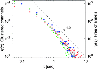 |
| | Fig. 5 Statistics of the waiting times measured in the motion of individual labelled potassium channels in the plasma membrane of living human kidney cells, combining the data of two different channel configurations, see ref. 50 for details. The asymptotic power-law trend of the waiting time distribution in this graph scales like ≃τ−1.9. Data courtesy Diego Krapf, Colorado State University. | |
In the theory of CTRWs one can readily show that the MSD with waiting time PDF (14) is subdiffusive and governed by eqn (8), where the generalised diffusion constant is defined via42,43
| |
 | (15) |
What is the dynamic equation connected to this CTRW process? On the stochastic level, the regular Langevin equation d
x(
s)/d
s =
ξ(
s) driven by the white Gaussian noise
ξ(
s) is augmented with a second equation
subordinating the number of steps
s to the real process time
t.
52–55 After averaging over the noise, in the diffusion limit we obtain the fractional diffusion equation,
42,56| |
 | (16) |
where we introduced the Riemann–Liouville fractional operator defined by
57,58| |
 | (17) |
In the limit
α = 1 we recover the normal diffusion
eqn (1). The fractional diffusion
eqn (16) can equivalently be formulated in terms of the Caputo operator.
58 In
eqn (17) we see that the process is dominated by the slowly decaying memory given by the integral over the power-law kernel. In the presence of an external potential, the dynamics is described in terms of the fractional Fokker–Planck equation.
42,59 This fractional Fokker–Planck equation fulfils a generalised form of the Einstein–Stokes relation as well as linear response.
42,59 We note that reactions in such a subdiffusive setting are discussed in
ref. 60. An interesting generalisation to evanescent CTRW subdiffusion was discussed recently.
61
As illustrated in Fig. 6, during the evolution of the process longer and longer waiting times emerge. Due to the lack of a characteristic time scale of ψ(τ), extreme individual waiting times τ arise which are of the same order as the measurement time. In particular, there is no longer a scale 〈τ〉 separating a single or a few jumps from the limit of many jumps. This effects a disparity between the MSD and the time averaged MSD, the so-called weak ergodicity breaking31,32,36,62–67
| |
 | (18) |
More specifically, as this subdiffusive process is no longer self-averaging such as the normal Brownian motion, to be able to obtain analytical results we introduce the additional averaging
| |
 | (19) |
over sufficiently many (more correctly,
N → ∞) individual trajectories. From a data analysis point of view, this procedure ensures smooth curves for

as function of the lag time
Δ.
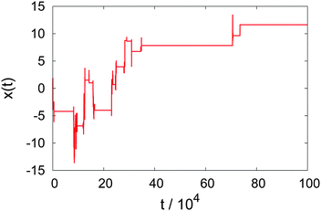 |
| | Fig. 6 Trajectory of a subdiffusive CTRW with waiting time PDF (14) and α = 1/2. In the evolving process longer and longer waiting times appear, a characteristic of the scale-free underlying law (14) of this non-stationary process. | |
Using the known fact that for subdiffusive CTRWs the average number of jumps from t = 0 up to time t scales like 〈n(t)〉 ≃ tα, it is quite straightforward to show that in the limit Δ ≪ t the result for the time averaged MSD is32,44,63,64
| |
 | (20) |
This is the first example of weak ergodicity breaking that we analyse in the following. Remarkably, the linear lag time dependence is different from the
tα-scaling of the MSD (8). Simultaneously, the length of the time series (measurement time)
t occurs explicitly in
expression (20). The latter echoes the ageing dependence of the subdiffusive CTRW process, to be addressed shortly in more detail: the longer the process lasts, the smaller the time averaged MSD becomes. Physically, this corresponds to the above observations that for the scale-free waiting time distribution
(14) longer and longer trapping times occur, stalling the progress of
x(
t). The linear form
(20) of the time averaged MSD was shown for the subdiffusive motion of lipid granules in living yeast cells,
68 and the ageing dependence

was observed for the motion of insulin granules in the cytoplasm and of potassium channels in the plasma membrane of living human cells.
50,69 For the channel motion in the plasma membrane the data are shown in
Fig. 7.
††
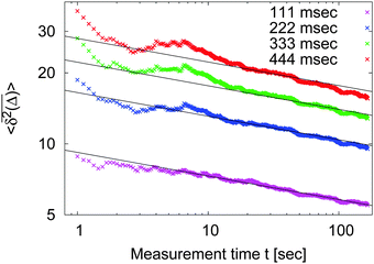 |
| | Fig. 7 Dependence of the time averaged MSD on the measurement time, observed for the motion of potassium channels in the plasma wall of human kidney cells in ref. 50. The straight lines show the scaling  with α = 0.9 deduced from the statistics of waiting times of this system shown in Fig. 5. The predicted scaling is nicely fulfilled by the data, corroborating the ageing nature of the system: the longer the system evolves (given by the times in the figure key) the smaller the apparent diffusivity. Data courtesy Diego Krapf, Colorado State University. with α = 0.9 deduced from the statistics of waiting times of this system shown in Fig. 5. The predicted scaling is nicely fulfilled by the data, corroborating the ageing nature of the system: the longer the system evolves (given by the times in the figure key) the smaller the apparent diffusivity. Data courtesy Diego Krapf, Colorado State University. | |
Note that the linearity of the time averaged MSD (20) for subdiffusive CTRWs may be deceiving: when such a linear scaling is observed for the time averaged MSD in experiments, it may easily be concluded that the observed process is normal. Without testing other quantities, such as the dependence of  on the measurement time t, such a conclusion may in fact be wrong. Note that in the limit α = 1 eqn (20) reduces to the ergodic Brownian form, independent of the trace length t.
Another a priori surprising result is that for confined subdiffusive CTRW motion the time averaged MSD does not converge to the thermal plateau. Instead, after engaging with the confinement it continues to grow in the power-law form45
| |
 | (21) |
where the prefactor involves the first two moments of the Boltzmann distribution,
| |
 | (22) |
of the confining potential
V(
x). The normalisation factor is given in terms of the partition function

. Only in the Brownian limit
α = 1, we observe a turnover from the free diffusion behaviour to a plateau with

. In the general case 0 <
α < 1 the time averaged MSD
(21) grows with
Δ, however, as long as
Δ ≪
t, the value of

never exceeds (〈
x2〉
B − 〈
x〉
B2).
‡‡ The behaviour
(21) was found from simulations in
ref. 70 and experimentally corroborated from optical tweezers tracking data in
ref. 68.
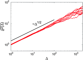
Each individual, sufficiently long time series of this subdiffusive CTRW process is characterised by a number of extremely long waiting times. However, in each realisation different numbers and lengths of such waiting periods occur. This gives rise to the fact that time averages remain random even for very long averaging times, and time averaged physical observables are thus irreproducible.45,64,73 This situation is shown in Fig. 8, where the simulation data show variations in the slope in individual  traces as well as a distinct amplitude scatter between different
  . Qualitatively these are reminiscent of the observations made in the experiments of Golding and Cox.§§33 Similar amplitude variations are observed in the aforementioned single particle tracking studies in living cells50,68,69,71 and in the simulation of associated water in the vicinity of lipid bilayers.72 We quantify this randomness of the time averaged MSD in terms of the dimensionless variable64
| |
 | (23) |
The associated distribution is
64,73| |
 | (24) |
for sufficiently long measurement times
t. Here
lα is a one-sided, completely asymmetric Lévy stable law with the Laplace image
![[script L]](https://www.rsc.org/images/entities/char_e144.gif)
{
lα(
t)} = exp(−
uα).
¶¶74 Note that the variable
ξ is in the denominator of the argument of
lα in
eqn (24), and thus moments 〈
ξn〉 exist. In particular, for
α = 1/2, the distribution of
ϕ(
ξ) is the half Gaussian
ϕ(
ξ) = (2/π)exp(−
ξ2/π), whose maximum occurs at
ξ = 0,
i.e., in very long trajectories the most likely case is that the amplitude

vanishes. For a fully ergodic process with
α = 1 the distribution has the sharp form
ϕ(
ξ) =
δ(
ξ − 1), which implies that individual trajectories are completely reproducible and there is no scatter in the relative amplitude
ξ around the ergodic value
ξ = 1. The variance of the amplitude fluctuations of

is measured in terms of the ergodicity breaking parameter
64,75| |
 | (25) |
which monotonically varies from EB = 1 for
α → 0 to EB = 0 for
α → 1. The latter mirrors the ergodic behaviour found for Brownian motion by Nordlund.
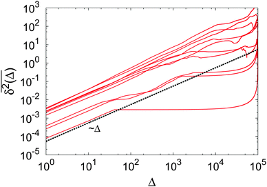 |
| | Fig. 8 Sample trajectories of a subdiffusive CTRW with power-law waiting time PDF (14) for α = 1/2. For 10 individual trajectories of length 105 (a.u.) we show the time averaged MSD (6). While the general slope of the time averaged MSD  follows the linear lag time dependence predicted by eqn (20), local deviations of the slope are visible. Moreover, the variation (scatter) of the amplitudes between different time traces is distinct. Both effects are due to the occurrence of long waiting times between jumps, due to the scale-free nature of ψ(τ), eqn (14). follows the linear lag time dependence predicted by eqn (20), local deviations of the slope are visible. Moreover, the variation (scatter) of the amplitudes between different time traces is distinct. Both effects are due to the occurrence of long waiting times between jumps, due to the scale-free nature of ψ(τ), eqn (14). | |
How can scale-free forms of the waiting time distribution (14) come about? Scher and Montroll explained this in terms of energetic traps in a quenched energy landscape as that shown in Fig. 9. When the depths of individual energy wells are exponentially distributed, the motion of a particle on this landscape is dominated by individual thermal escapes from these traps characterised by the Kramers/Arrhenius activation, only to be trapped again in the next well. As the motion of the particle progresses, it typically encounters ever deeper wells, effecting the subdiffusive behaviour.39 This scenario indeed gives rise to the waiting time PDF (14).||||37,76 The correspondence of the Arrhenius-type escape in the energy landscape to power-law waiting time distributions renders the CTRW an extremely successful mathematical model for the description of the mechanisms of anomalous diffusion in a number of important physical systems.
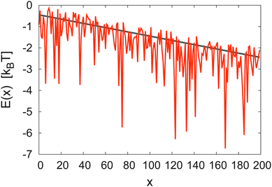 |
| | Fig. 9 Quenched trap model with constant bias.39 We show a realisation of the trapping landscape with exponential distribution p(E) = Tg−1exp(−E/Tg) of trap depths E, where we set the Boltzmann constant to unity. The system specific “glass” temperature Tg (here, Tg = 1) sets the width of p(E). We also include a unit tilting force. On its way through this landscape, a random walker successively falls into traps and faces escape times given by Arrhenius' law τ ≃ exp(E/T), where T is the temperature of the thermostat. Due to the tilt, revisits to a given trap are unlikely, and the model thus corresponds to an annealed (biased) continuous time random walk with power-law waiting time PDF (14) with α = T/Tg. When the system temperature is below Tg, subdiffusion is effected. | |
Alternative sources for the power-law form (14) are spatial traps. One example is the Havlin–Weiss comb model originally designed to mimic the spatial trapping of particles in the dangling ends of a percolation cluster:77 a particle moves along the x axis but can get transiently trapped in perpendicular one-dimensional channels, a structure similar to the teeth of the comb. As the returning probability scales like t−1/2, the effective motion along the x axis is governed by the waiting time PDF (14) with α = 1/2. This exponent is indeed observed in typical experiments of tracer dynamics in subsurface aquifers and may correspond to the trapping of tracer molecules in thin cracks off the main water artery.78 Further examples of systems leading to a power-law form of ψ(τ) are dynamic maps79–84 and the sticking of tracer particles around stable islands of weakly chaotic systems.***51,85
Ageing effects of the subdiffusive CTRW. Power-law distributed waiting times lead to ageing in a wide variety of systems. Suppose you observe the on–off blinking of a single, illuminated quantum dot between a light emitting and a dark state.34 While such an experiment will show many rapid transitions between the on and off states, occasionally very long on or off periods will appear. Over a sufficiently long observation period t, the duration of these long events typically increases with t.34 A similar effect is observed for the motion of potassium channels in the plasma membrane of living cells50 or for the diffusion of submicron tracers in a cross-linked actin mesh:48 longer and longer immobilisation periods occur in the course of the measurement. We already alluded to this phenomenon in the discussion of the CTRW trajectory in Fig. 6 and from Fig. 7. Such strongly non-stationary, out-of-equilibrium behaviour is indeed well known from glassy systems,76,86 a field in which the term ageing was originally coined. Subdiffusive CTRWs are non-stationary, as we could see from the explicit dependence of  on the measurement time t in eqn (20), and they have been proposed to capture the observed dynamics in glassy systems.87
What if we start to probe such an ageing system only at some (ageing) time taafter the system was initially prepared at time t = 0? As the subdiffusive CTRW evolves, on average longer and longer waiting time events appear in the trajectory (compare the time trace in Fig. 6). When we start to observe the particle we will typically find it within one of the extremely long waiting periods. The occurrence of the first step in this scenario is no longer determined by the statistics of the waiting time distribution ψ(τ) from eqn (14) but occurs at the forward waiting (recurrence) time t1 (see Fig. 10), which is governed by the PDF73,88–90
| |
 | (26) |
At longer ageing times (
ta ≫
t1), the scaling
h(
t1,
ta) ≃
t−α1 in terms of
t1 of the forward waiting time PDF is thus broader than that of the original waiting time PDF
(14),
ψ(
τ) ≃
τ−1−α. Due to the memory of the CTRW process—directly visible in the fractional diffusion
eqn (16)—strong ageing persistently affects the time evolution of the process.
 |
| | Fig. 10 Schematic of the forward (recurrence) waiting time. A process governed by the waiting time PDF (14) is started at t = 0. Events (jumps of a random walker or on–off transitions of a blinking quantum dot) are symbolised by the blue impulses. When we start to follow the system's dynamics after the ageing period at ta, the forward waiting time until the first jump occurs is t1. | |
The behaviour of the MSD for free, unconfined CTRW motion in this ageing scenario then exhibits the crossover73,89
| |
 | (27) |
which for strong ageing (
ta ≫
t) shows an apparent linear scaling with time
t. Only when the process evolves for much longer than the original ageing time,
t ≫
ta, the scaling with
t reflects the subdiffusive nature of the process.
Remarkably, the behaviour of the associated time averaged MSD
| |
 | (28) |
is much more transparent in the presence of ageing. Namely, in the limit
Δ ≪
t the result is
73| |
 | (29) |
where the right hand side involves the non-aged quantity

. The physical scaling with the lag time
Δ is not affected, and all information on the ageing enters as the ratio
ta/
t into the universal algebraic prefactor
| | |
Λ(z) = (1 + z)α − zα.
| (30) |
As shown in
ref. 73, this
ageing depression also occurs for other time averaged physical observables. In contrast to the ensemble average, the scaling with
Δ is the same for any ageing time
ta, and thus time averages are in that sense more suitable measurables for aged systems. Finally, we remark that in the limit of strong ageing
ta ≫
t ≫
Δ, we even obtain an equivalence of the limiting behaviour of the regular MSD and the time averaged MSD,
73| |
 | (31) |
Another important lesson to be drawn from ageing renewal theory73,89 is the fact that in a growing fraction of trajectories no jump occurs within the observation window from the ageing time ta to ta + t. It was shown in ref. 73 that the probability to have a nonzero number of steps during this observation window decays as mα ≃ (t/ta)1−α for strong ageing ta ≫ t. Concurrently the discrete probability for not moving at all during the observation grows. Observing a series of individual particles, one therefore finds a population splitting into mobile and immobile particles.73 This fact is important when one wants to extract the amplitude—for instance, the anomalous diffusion coefficient Kα—from a given set of time averaged data.73 Notably, also the scatter distribution ϕ(ξ) is significantly altered.73 The splitting into mobile and immobile fractions may be underlying the experimentally observed population splitting in molecular biological systems.91Fig. 11 demonstrates for the same number of simulated trajectories how ageing suppresses the mobile fraction of particles within the observation window ta…ta + t.73
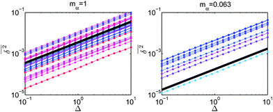 |
| | Fig. 11 Time averaged mean squared displacement  for individual free CTRW trajectories (full symbols) and the averages according to eqn (29) (bold black lines). Left: non-aged system with mα = 1. Right: aged process, ta = 1011 (a.u.), in which the large fraction 1 − mα ≈ 94% of trajectories is suppressed in the log–log plot. The parameters are α = 1/2, 〈δx2〉 = 1, 〈τ〉 = 1, and t = 109. Compare ref. 73. for individual free CTRW trajectories (full symbols) and the averages according to eqn (29) (bold black lines). Left: non-aged system with mα = 1. Right: aged process, ta = 1011 (a.u.), in which the large fraction 1 − mα ≈ 94% of trajectories is suppressed in the log–log plot. The parameters are α = 1/2, 〈δx2〉 = 1, 〈τ〉 = 1, and t = 109. Compare ref. 73. | |
Ageing also affects other quantities of the subdiffusive CTRW process, for instance, the first passage behaviour. Thus, for unbiased subdiffusion on a semi-infinite domain the density of first passage times acquires the three distinct scaling regimes92
| |
 | (32) |
with the time scale
t* ≃
t1+α/2aK1/2α/
x0 containing the initial distance
x0 between the particle and the absorbing boundary. As expected, as long as ageing is weak, the scaling of the first passage time PDF with
t features the exponent (−1 −
α/2) of the non-aged system.
42,93,94 However, as ageing becomes more severe, there exists a competition between the magnitudes of the ageing time
ta and the measurement time
t, with the intermediate scaling exponent (−1 −
α) and the fully aged exponent (−
α). In particular, the intermediate scaling is steeper than for both the non-aged and the fully aged system. This observation, in principle, offers the possibility to determine the age
ta of the system from observation of the first passage behaviour, albeit sufficiently many and long trajectories are needed to evaluate

.
92
We so far discussed the case with 0 < α < 1, when the characteristic waiting time 〈τ〉 diverges. What happens when 〈τ〉 is finite but the fluctuations around it diverge, i.e., for the case 1 < α < 2? It can be shown that indeed the process in many facets is different from the naively expected Brownian behaviour. Instead, different ageing features characterise the process.95,96 To fully understand the consequences on quantities such as the time averaged MSD  or its amplitude scatter, more work is needed.
3.2 Noisy continuous time random walks
In the subdiffusive CTRW the particle becomes fully immobilised with respect to the co-ordinate x(t) in between successive jump events (see Fig. 6). For charge carriers in an amorphous semiconductor or for tracer particles firmly stuck to much larger objects or solid surfaces this assumption appears to be reasonable. However, imagine a submicron tracer particle in a cross-linked network consisting of semi-flexible actin filaments.48 In this case the particle is stuck in cages for waiting times distributed like the power-law (14). The actual trajectory shows distinct fluctuations of approximately constant amplitude around a mean location.48 This behaviour stems from the thermal nature of the system, that is, the cages in the mesh are typically somewhat larger than the tracer particle and/or the actin filaments making up the mesh are themselves subject to thermal agitation, compare the results of recent simulations of tracer motion in a flexible gel.97 In the noisy CTRW the superimposed noise is combined with the fully immobilised periods of the native CTRW.98 This model is therefore relevant for the quantitative description of the stochastic particle motion in a large range of systems. In particular, a detailed analysis of recorded data in terms of the noisy CTRW may unveil an underlying power-law waiting time despite the fact that no clear stalling events feature in the measured trajectory.
In the above scenario of approximately constant amplitude noise around the horizontal immobilisation periods in the x(t) diagram, it is a natural choice to add Ornstein–Uhlenbeck noise in the position space to the native subdiffusive CTRW process (see Fig. 12). For the MSD this leads to the additive terms98
| |
 | (33) |
where the first term represents the contribution of the native CTRW. The second term contains the noise strength
η2D made up of the diffusivity
D of physical dimension cm
2 s
−1 and the empirical noise amplitude
η. This dimensionless noise strength should not be confused with the friction coefficient used earlier. Moreover,
k is an inverse time scale governing the relaxation of the Ornstein–Uhlenbeck process to stationarity. The Ornstein–Uhlenbeck component in the MSD
(33) after the time scale 1/
k becomes merely an additive constant, whose relative amplitude becomes progressively smaller compared to the first term. The effect on the trajectory itself is displayed in
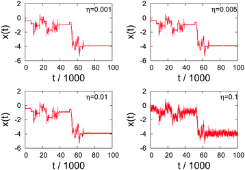
Fig. 12: for increasing noise amplitude the stalling periods of the native CTRW become more and more masked and resemble the experimental trajectories of the submicron tracers in the semi-flexible polymer network.
48 The results for the MSD are shown in
Fig. 13.
 |
| | Fig. 12 Noisy CTRW process with Ornstein–Uhlenbeck noise with α = 0.8, for different amplitudes η of the superimposed Gaussian noise. Increasing η washes out the immobilisation periods of the pure CTRW process. | |
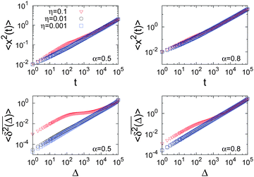 |
| | Fig. 13 Ensemble averaged (top) and time averaged (bottom) MSDs for the noisy CTRW process.98 In each case we present results for α = 0.5 and α = 0.8 for three different noise strengths. The trajectory lengths are t = 105, and the symbols represent an average over 103 trajectories. | |
The associated time averaged MSD becomes98
| |
 | (34) |
in absence of ageing (
ta = 0). In contrast to the MSD
(33), the time averaged MSD
(34) contains the factor
tα−1 in the first term representing the native CTRW contribution, while the amplitude of the noise in the second term on the right hand side is independent of
t. While for small noise amplitude
η the observable

will essentially be indistinguishable from the native CTRW, for larger
η we observe a distinct crossover behaviour for

. Namely, for shorter lag times the time averaged MSD shows contributions from both the native CTRW and the Ornstein–Uhlenbeck noise. Writing

, for
Δ ≪ 1/
k we find
Dapp ≃
Kαtα−1/
Γ(1 +
α) +
η2D. At longer lag times, solely the native CTRW contribution is visible and
Dapp ≃
Kαtα−1/
Γ(1 +
α). In between these two regimes, a crossover behaviour is observed, as shown in
Fig. 13. However, when the measurement time
t is much longer than the lag time
Δ, the Ornstein–Uhlenbeck term is dominant. Again the time average has a clear advantage over the ensemble average, as it reveals additional detail of the behaviour.
A different scenario can also be envisaged.98 For instance, when the observer is interested in the motion of a tracer inside a living cell and the attachment of the cell to the cover slide in the microscope turns out to be broken, the data will show the additional Brownian noise stemming from the random cell motion superimposed to the anomalous motion with respect to the reference frame of the cell. In that case the MSD reads98
| |
 | (35) |
which exhibits a turnover from the subdiffusive scaling with
tα to the linear Brownian growth ≃
t in the long time limit. The associated time average is always linear,
98| |
 | (36) |
We note that the superposition of Poissonian and non-Poissonian noise was also discussed in a biologically inspired reaction rate model.99
3.3 Ultraslow diffusion of continuous time random walks in an ageing environment
The subdiffusive CTRW process discussed so far is a renewal process. That is, after each step the waiting time τ is randomly chosen from the same PDF ψ(τ). Physically, this corresponds to an annealed environment.39 More formally, one can view this process as if the random walker carried his own clock around whose random ticks trigger the occurrence of the jumps. As we discussed above, if we want to describe an aged subdiffusive CTRW initiated at t = 0 and evolving for the ageing time ta, the statistics for the occurrence of the first jump in an observation beginning at ta is modified. The first jump occurs after the forward waiting time t1, which is distributed with the probability density function (26). All subsequent waiting times are then again drawn from the standard law (14).
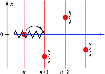
Here we consider a different scenario, in which each jump event depends on the present age of the system. Imagine a toy scenario for a rupture model, in the spirit of Zener's famous work on stress relaxation in solids:100 a crack in a two-dimensional material is propagating along the discrete n axis, as sketched in Fig. 14. The crack is represented by the bold black zig-zag line. As indicated by the arrow, this crack has just propagated from site n to n + 1. Crack propagation is triggered by the red circles (the ‘vacancies’), which diffuse along the perpendicular x axis. When the vacancy at site n hit the x = 0 line the crack tip was allowed to extend to site n + 1. To propagate to site n + 2, the vacancy at n + 1 has to diffuse to x = 0, etc. If the vacancies can only diffuse along a finite interval of length ![[small script l]](https://www.rsc.org/images/entities/char_e146.gif) on the x-axis, they return to x = 0 on time scales τx ≃
on the x-axis, they return to x = 0 on time scales τx ≃ ![[small script l]](https://www.rsc.org/images/entities/char_e146.gif) 2. This τx then is the average time for the crack propagation from one site to the next, and we will find the crack propagation law 〈n(t)〉 ∼ t/τx.
2. This τx then is the average time for the crack propagation from one site to the next, and we will find the crack propagation law 〈n(t)〉 ∼ t/τx.
 |
| | Fig. 14 Sketch of the crack propagation model discussed in the text. The tip of the crack (black zig-zag line) propagates from site n to n + 1 when the vacancy represented by the red circle diffuses to the origin (x = 0) at point n. | |
What happens if the length ![[small script l]](https://www.rsc.org/images/entities/char_e146.gif) becomes very large and the vacancies can venture far away? As known from the theory of comb models,77 the probability density of return to x = 0 is of power-law form, proportional to τ−1
becomes very large and the vacancies can venture far away? As known from the theory of comb models,77 the probability density of return to x = 0 is of power-law form, proportional to τ−1![[thin space (1/6-em)]](https://www.rsc.org/images/entities/char_2009.gif) −
−![[thin space (1/6-em)]](https://www.rsc.org/images/entities/char_2009.gif) 1/2. Typically, when the tip of the crack reaches a new site, the vacancy will be away from x = 0, and the triggering event for the crack propagation to the next site then corresponds to the forward waiting time t1 distributed according to eqn (26) with α = 1/2. In contrast to the previously discussed renewal ageing CTRWs, however, the next propagation step of the crack tip again occurs with the forward waiting time, characterising the arrival of the next vacancy at x = 0, and so forth. In other words, every step occurs with the forward waiting time t1. The probability that the tip arrives at an extremely long forward waiting time t1 increases considerably.††† This fact significantly alters the dynamics of the process. Formally, this scenario corresponds to a random walker, which is updated by stationary, site-specific clocks.
1/2. Typically, when the tip of the crack reaches a new site, the vacancy will be away from x = 0, and the triggering event for the crack propagation to the next site then corresponds to the forward waiting time t1 distributed according to eqn (26) with α = 1/2. In contrast to the previously discussed renewal ageing CTRWs, however, the next propagation step of the crack tip again occurs with the forward waiting time, characterising the arrival of the next vacancy at x = 0, and so forth. In other words, every step occurs with the forward waiting time t1. The probability that the tip arrives at an extremely long forward waiting time t1 increases considerably.††† This fact significantly alters the dynamics of the process. Formally, this scenario corresponds to a random walker, which is updated by stationary, site-specific clocks.
If we generalise the CTRW model and consider a process in which every jump occurs with the waiting time PDF (14) with general 0 < α < 1, it can be shown that the crack propagation dynamics is reduced to the much slower logarithmic law101
| |
 | (37) |
where
μ = −
Γ′(
α)/
Γ′(
α) −
![[small gamma, Greek, macron]](https://www.rsc.org/images/entities/i_char_e0c4.gif)
in terms of the complete
Γ function and its derivative
Γ′,
![[small gamma, Greek, macron]](https://www.rsc.org/images/entities/i_char_e0c4.gif)
= 0.5772… is Euler's constant, and
t0 is a cutoff time to avoid divergencies at
t = 0. The counting process
n(
t) is deterministic in the sense that the relative fluctuations
| |
 | (38) |
albeit slowly, decrease during the progress of time.
101 For
α > 2 the process is normal and statistically equivalent to a Poisson update, which is equivalent to the above scenario with finite length
![[small script l]](https://www.rsc.org/images/entities/char_e146.gif)
for the vacancy diffusion leading to the linear time dependence 〈
n(
t)〉 ≃
t. However, similar to our observations above, the case with a finite characteristic update time 〈
τ〉 but diverging variance of waiting times with 1 <
α < 2 displays the power-law anomaly 〈
n(
t)〉 ≃
tα−1.
101
Interestingly, the time average over the time series n(t),
| |
 | (39) |
is linear in the lag time
Δ, in analogy to the results
(20) for the regular renewal subdiffusive CTRW process. The inverse dependence on the measurement time
t with the logarithmic correction observed here, in a rough way can be viewed as the
α → 0 behaviour of the power-law relation in
eqn (20).
Above we constructed the crack propagation model such that the motion of the tip is fully biased and each step is directed to higher n values. What if we interpret the update rule for the counting dynamics n(t) as jumps of a random walk process in real space? To avoid correlations when the random walker revisits the same spatial point and its next update is governed by the same clock as during the previous visit, in analogy to the discussion of the quenched trap model we could include a spatial bias of the random walk. Alternatively, we could embed the random walk in three dimensions. Due to the transient nature of this process, revisits are significantly reduced, and the MSD
of the walker is then proportional to 〈
n(
t)〉, while the corresponding time averaged MSD
| |
 | (41) |
scales like

. Such a random walk process thus exhibits weakly non-ergodic behaviour.
The random walk process in an ageing environment corresponds to a non-renewal process in dimension one and two. In dimension three it is a renewal process, however, here the waiting time distribution (14) is replaced by the PDF of the forward (recurrent) waiting time. In other words, due to the logarithmic nature the process, eqn (37), can be shown to be governed by the limiting distribution for the product of independent random variables, the log-normal distribution.101 This approach may thus be of relevance to a large range of applications in which this distribution is identified.102
In the regular, renewal subdiffusive CTRW ageing affects the statistics of the first jump, given in terms of the forward waiting time t1. All subsequent jumps occur with the regular waiting time PDF (14). The system remembers the first step, due to the slowly decaying memory inherent to the process, seen in the non-local time operator of the associated fractional diffusion eqn (16). Once the process time exceeds the ageing time significantly, i.e., t ≫ ta, the ageing effects are no longer visible.‡‡‡ In the non-renewal scenario discussed here the system has a high likelihood to encounter atypically long waiting times at every step and thus every single step includes ageing. This causes the massive retardation of the motion, giving rise to the emerging logarithmic law. Such time dependencies occur in a large variety of systems, inter alia, the crumpling of paper,103 compactification of grains,104 or record statistics.105 Recently, it was shown that the long time behaviour of a tracer particle in a single file system, in which individual particles repel each other and may stick to a functionalised channel with power-law waiting times, can indeed be described in terms of the logarithmic time dependence derived here within the non-renewal ageing process.106
Other ultraslow diffusion processes. In the theory of stochastic processes, the logarithmic time evolution has a prominent representative, namely, Sinai diffusion.107 In this special case of Temkin's model,108 the random walker moves in the quenched energy landscape created by a seed random walk. Thus, locally the walker experiences a force of the same amplitude, randomly to the left or the right. The walker can become trapped significantly when the bias in a number of adjacent sites points in the direction of the walker's current location. To get to a distance x from its starting point the particle needs to cross an energy barrier of the typical order  , corresponding to an activation time scale
  , where τ1 is a fundamental time scale and c a dimensional constant. The typical distance covered by the walker during time t then scales according to the ultraslow, logarithmic law x2 ≃ log4(t/τ1),39 compare also the discussion in ref. 109. Referring to ref. 110 for further explanations, we quote the result for the time averaged MSD
| |
 | (42) |
where the tilde denotes the disorder average. Interestingly, also here the time averaged MSD increases linearly with the lag time and exhibits a strong sensitivity to the measurement time. A generalisation of the Sinai model with strongly correlated disorder113 and a periodic Sinai model111 were reported recently. The splitting probability of the Sinai model is determined in ref. 112.In terms of a renewal CTRW ultraslow processes can be established by using a waiting time PDF of the form ψ(t) ≃ 1/(t![[thin space (1/6-em)]](https://www.rsc.org/images/entities/char_2009.gif) log1+γt),110,114–116 which is normalised but does not possess finite moments of any power 〈τq〉 with q > 0. It produces an MSD of the form
log1+γt),110,114–116 which is normalised but does not possess finite moments of any power 〈τq〉 with q > 0. It produces an MSD of the form
| |
〈x2(t)〉 ≃ log![[thin space (1/6-em)]](https://www.rsc.org/images/entities/char_2009.gif) γt, γt,
| (43) |
i.e., for
γ = 4 the MSD scales identically to that of the Sinai diffusion. The weakly non-ergodic behaviour of ultraslow CTRWs is analogous to
eqn (42) for Sinai diffusion, apart from the general exponent
γ and the prefactor,
| |
 | (44) |
The time averaged MSD, the localisation of the diffusion particle, as well as the ergodic properties of both Sinai and ultraslow CTRW diffusion are analysed in
ref. 110, discussing some of the fundamental differences between time averages recorded in annealed
versus quenched environments.
Finally, ultraslow diffusion can also be effected by iterative dynamics maps, as shown by Dräger and Klafter.116 Instead of the power-law maps with a single exponent z discussed in ref. 79, however, ultraslow diffusion emerges when an entire hierarchy of exponents is considered. In very dense two-dimensional lattice gas systems, ultraslow diffusion emerges, as well.117
3.4 Correlated continuous time random walks
Another way to break the renewal character of the standard CTRW process is to introduce correlations between successive waiting times. Correlations appear naturally in the motion behaviour of higher animals or humans, or in the dynamics of financial markets. They are also present for particles diffusing in quenched disorder, compare the above discussion of the quenched trap model or Sinai diffusion. It is therefore consequent to consider non-renewal CTRW processes with built-in correlations. This can be achieved by extension of the subordination of the physical time to the number of steps of the process.118,119 An alternative approach is the following.
Assume that successive waiting times are correlated in a way that waiting time τi is given by waiting time τi−1 modified by a small increment, δτi, that is, τi = τi−1 + δτi. The increments δτi may be positive or negative. Successive waiting times are thus correlated: a short waiting time is followed by a similarly short one, and vice versa for a long waiting time. This approach corresponds in fact to a random walk in the space of waiting times, and we can write the current waiting τi time as the sum of increments120–123
| | |
τi = |δτ0 + δτ2 + … + δτi|.
| (45) |
The absolute value occurs here as waiting times always have to be positive. These increments
δτi are then chosen to follow a given probability distribution. We may, for instance, consider the symmetric Lévy stable law defined in terms of its Fourier transform as exp(−
cγ|
k|
γ). The process can then be shown to produce a power-law MSD of the form
(8) with anomalous diffusion exponent
| |
 | (46) |
whose range spans from zero (for
γ = 0) to 2/3 (for
γ = 2) and thus leaves a gap to normal diffusion.
120,121 Brownian motion with
α = 1 in this model can only be restored by completely breaking the correlations.
120 In the limit
γ = 2 the mode relaxation is of stretched exponential form,
P(
k,
t) ≃ exp(−
ct1/2), and for the range 0 <
α < 2 it is of power-law shape, ≃
t−α.
122
Fig. 15 compares the CTRW model with correlated waiting times (45) with the regular subdiffusive CTRW. In the correlated case the gradual increase of the waiting times is distinct from the occasional very long waiting times of the uncorrelated model. Also the trajectories of the two models are very different: without correlations, the long waiting times effect distinct immobilisation events, while for the correlated waiting times, the motion appears almost Brownian, albeit with a gradual increase of the waiting times.
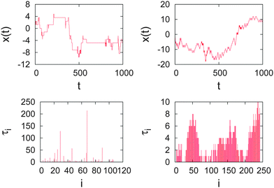 |
| | Fig. 15 Trajectory x(t) (top) and individual waiting times (bottom) in the regular subdiffusive CTRW model with α = 2/3 (left) and the CTRW model with correlated, Gaussian waiting times256 with γ = 2 (right). Both cases lead to the same MSD (8) with α = 2/3. | |
In this process the waiting time on average is an increasing function and diverges in the limit of many steps. The correlated CTRW process indeed exhibits weakly non-ergodic behaviour,122
| |
 | (47) |
such that the range of the ageing exponent 1 −
γ/(1 +
γ) is in between 1/3 and one. Moreover the process ages, as shown
via the decaying response of the process to a sinusoidal driving force.
122
Similarly, when the waiting times are exponentially distributed but the jump lengths correlated the process leads to the exact form120
| | |
〈x2(t)〉 = ¼K3(t(t + 1)(2t + 1)) ≃ K3t3
| (48) |
of superdiffusive behaviour with the asymptotic cubic Richardson form
26 when the distribution of jump length increments is Gaussian. When the jump length increments are drawn from a Lévy stable law with index
μ, the MSD diverges. From fractional oder moments one can derive the scaling relation
x2 ∼
t(1+μ)/μ. For the case
μ = 2 the weakly non-ergodic form of the MSD
| |
 | (49) |
was obtained exactly, and the expansion is valid for
Δ ≪
t.
120
3.5 Superdiffusive continuous time random walks and ultraweak ergodicity breaking
For completeness we also consider superdiffusive renewal CTRW processes. To that end we note that the introduction of a waiting time distribution into a standard random walk process at most leads to a subdiffusive behaviour when the first moment of the waiting time PDF ψ(τ) diverges. Superdiffusion cannot be achieved within the approach of a generalised waiting time concept. There exist, however, two pathways to extend the CTRW model to superdiffusion.
The first way is to modify the distribution of jump lengths. All CTRW processes considered so far (apart from the case of correlated jump lengths in the preceding section) correspond to the motion on a lattice, or in continuous space with a jump length PDF that possesses a finite variance 〈δx2〉 and zero mean 〈δx〉. What if we choose a jump length distribution λ(δx), for which the variance 〈δx2〉 diverges? Consider a Lévy stable form with the asymptotic power-law behaviour λ(δx) ≃ 1/|δx|1+μ of the jump lengths with the stable index 0 < μ < 2. When the waiting time PDF has finite moments, this process was called a Lévy flight by Mandelbrot.124 The divergence of the jump length variance translates into the divergence of the second moment of the PDF P(x,t),125 and only fractional order moments 〈|x|κ〉 with 0 < κ < μ exist.42 The trajectory of a Lévy flight is fractal (see below) of Hausdorff dimension μ. A single trajectory therefore never fully covers an embedding space whose dimension is larger than μ. This is particularly relevant in the two-dimensional world, in which effectively most human and animal motion occurs. There exist also several studies considering the combination of a diverging characteristic waiting time 〈τ〉 with a Lévy stable distribution of jump lengths, either in terms of fractional diffusion equations126 or via using subordination arguments.127 Due to its fractality a single Lévy flight trajectory cannot visit all points in space when the stable index μ is smaller than the embedding dimension d. Under confinement to a finite area, Lévy flights are ergodic,128 and the convergence to the ergodic state can be analysed in terms of the apparent fractal dimension or in terms of the first passage dynamics.129 The divergence of 〈δx2〉 as well as the ensuing non-ergodicity of Lévy flights can be rectified by a cutoff in the jump length PDF130 or by dissipative non-linearities.131 Such stochastic processes behave like a Lévy flight until the regularisation of the jump length PDF comes into effect.
The alternative approach is to introduce a coupling between jump lengths and waiting times. In subdiffusive CTRWs described previously the waiting time and jump length PDFs enter in the multiplicative form ψ(δx,τ) = ψ(τ)λ(δx).43 Introducing a functional dependence between waiting times τ and jump lengths δx, this spatiotemporal coupling preserves the renewal properties of CTRW processes but due to penalising long jumps—associating them with long waiting times—yields a finite MSD.43,132 The simplest choice is the coupling ψ(δx,τ) = ½ψ(τ)δ(|δx| − ντ), in which the velocity v is introduced. It bestows a propagating horizon to the process in the form of two travelling δ peaks with decaying amplitude. For waiting time PDFs ψ(τ) ≃ τ−1−α with 1 < α < 2, in between these peaks, a Lévy stable distribution is building up.133 Also Lévy walks are non-ergodic, albeit in a way, that is different from the above discussed non-ergodic behaviour.
To see this, we first recall that for a waiting time PDF of the power-law form ψ(τ) ≃ τ−1−α their MSD scales134,135
| |
 | (50) |
The associated time averaged MSD in the ballistic phase with 0 <
α < 1 scales like
| |
 | (51) |
with a higher order correction scaling with
Δ2(
Δ/
t)
2−α.
136,137 In the enhanced diffusion phase 1 <
α < 2 the result is
136–138| |
 | (52) |
In both the ballistic and enhanced diffusive phases the MSD differs from the time averaged MSD merely by a factor of 1/|
α − 1|. This phenomenon may be referred to as ultraweak ergodicity breaking.
138 Note that an analogous result was obtained by Zumofen and Klafter for Lévy walks with stationary and non-stationary initial conditions,
139 compare the discussion in
ref. 138. To leading order, the time averaged MSDs
(51) and (52) do not exhibit ageing in the sense that the measurement time
t does not appear explicitly, in contrast to the corresponding forms for the subdiffusive CTRW processes discussed above. Further physical properties of Lévy walks, in particular, the amplitude scatter of the time averaged MSD, are studied in
ref. 138 and 140 Additional recent studies of Lévy walks analyse their response to an external bias and the power spectral properties.
136–138,140
Lévy flights and walks are used as statistical models in many fields, for example, to quantify blind search processes of animals for sparse food.141–143 In the science of movement ecology, the so-called Lévy foraging hypothesis has become widely accepted.141 Recently this model was qualified for human motion behaviour and when different search criteria and external forcing are considered.144 These stochastic processes also describe the propagation of visible light in disordered optical media145 and the dynamics of quantum dots.34 In optical lattices the divergence of the position of single ions was shown to follow Lévy statistics.146 For more details compare also Section 7.
4 Fractional Brownian and Langevin motion
Next to the CTRW model, fractional Brownian motion (FBM) and the motion governed by the fractional Langevin equation (FLE) represent the second major stochastic models for the description of anomalous diffusion processes both in the presence and in the absence of external potentials. Physically, these types of motion arise when we observe the effective motion of a single tracer particle in a coupled many-body system such as a single file of excluded volume particles, see below.
4.1 Fractional Brownian motion
We believe that FBMs do provide useful models for a host of natural time series and wish therefore to present their curious properties to scientists, engineers and statisticians, argue Mandelbrot and van Ness in their defining work on FBM.147 The motivation for this study and Mandelbrot's earlier work148 were Hurst's laws for the discharge of the Nile and other rivers.149 In the Russian literature Kolmogorov introduced an analogous process already in 1940150 which was then analysed further by Yaglom.151 Mathematically, FBM indeed has curious properties,147 as it is not a semimartingale and cannot be interpreted in terms of a random walk process.152,153 Despite the many studies on FBM and its wide application in various fields of science, engineering, and beyond, many fundamental properties of FBM remain elusive, such as the first passage properties.154,155 At the same time FBM is distinguished by the fact that it is the only self-similar Gaussian process with stationary increments.147 Note that for notational consistency in the following we use the anomalous diffusion exponent α in the formulation of the fractional Gaussian noise which is related to the Hurst exponent H commonly used in the FBM literature via α = 2H.
Mandelbrot and van Ness define FBM in terms of the stochastic integral147
| |
 | (53) |
where
B(
t) is ordinary Brownian motion. A more intuitive representation uses the Langevin equation
| |
 | (54) |
which is fuelled by the fractional Gaussian noise
ξfGn(
t). The latter has a standard normal distribution for any
t > 0 but is power-law correlated,
§§§| | |
〈ξfGn(t1)ξfGn(t2)〉 = α(α − 1)Kα*|t1 − t2|α−2
| (55) |
for
t1,
t2 > 0 and
t1 ≠
t2. The physical dimension of
ξfGn(
t) is thus [
ξfGn] = cm s
−1. Due to the factor (
α − 1) the fractional Gaussian noise is
persistent or positively correlated for the case 1 <
α < 2, and it is
antipersistent or negatively correlated for 0 <
α < 1. The PDF for free FBM is given by the Gaussian
| |
 | (56) |
The position autocorrelation of FBM is
| | |
〈x(t1)x(t2)〉 = Kα*(tα1 + tα2−|t1 − t2|α),
| (57) |
and reduces to the MSD
(8) for
t =
t1 =
t2. From this quantity we can obtain the time averaged MSD
156| |
 | (58) |
showing that FBM is ergodic in the sense that is equivalent to the MSD
(8). As the process is self-averaging, for sufficiently long measurement times we even obtain the single trajectory equality, formally,
| |
 | (59) |
demonstrated in
ref. 156 and 157. As shown in
ref. 156, ergodicity is reached algebraically slowly, a property shared with that of regular Brownian motion (see also Section 4.3). For finite trajectory length
t the scatter distribution of the relative amplitude

can be approximated by the Gaussian
158| |
 | (60) |
where
τ* is a binning time scale.
Fig. 16 shows the reproducibility of unconfined FBM. Note that the scatter for longer lag times
Δ →
t is due to insufficient statistics of the time average.
 |
| | Fig. 16 Time averaged MSD  as a function of the lag time Δ for FBM with α = 0.5. Individual trajectories provide quite reproducible results, no significant scatter of the amplitude between different as a function of the lag time Δ for FBM with α = 0.5. Individual trajectories provide quite reproducible results, no significant scatter of the amplitude between different  arises, and the anomalous scaling arises, and the anomalous scaling  is fulfilled. is fulfilled. | |
4.2 Fractional Langevin equation motion
The FLE for the position co-ordinate x(t) of a particle with mass m is written as157,159–161| |
 | (61) |
where γ* is a friction coefficient of physical dimension [γ*] = g s−α and ξfGn(t) represents the fractional Gaussian noise (55) with 1 < α < 2.
The FLE (61) is a special form of the Hänggi–Kubo generalised Langevin equation160,162,163 driven by noise, which is not white but correlated. In contrast to the δ-correlated white noise encountered in the Langevin eqn (5), that is, the correlation function of the noise at time t explicitly depends on past times t′ < t with a given weight function. Concurrently, the friction term becomes a convolution integral such that the noise kernel balances the non-local noise to fulfil the generalised fluctuation dissipation relation.160,162,163 Such equations with memory arise in the Mori-Zwanzig projection operator framework.164 The FLE corresponds to the special case for which the noise autocorrelation is given by the power-law decay of the fractional Gaussian noise ξfGn(t). The friction kernel is then equally of power-law form.
The Kubo generalised fluctuation dissipation relation fixes the noise amplitude in the form
| |
 | (62) |
Typically, in single particle tracking experiments one observes the overdamped motion of the tracer. Such overdamped motion corresponds to neglecting the inertia term in
eqn (61), producing the overdamped FLE
| |
 | (63) |
The convolution integral can be replaced with the Caputo time fractional derivative
¶¶¶| |
 | (64) |
which then constitutes the
fractional Langevin equation
159| |
 | (65) |
or the corresponding overdamped FLE. Note that due to the coupling of the friction kernel and the fractional Gaussian noise
via the fluctuation dissipation relation a large instantaneous value of the noise couples to a high effective friction. For this reason fractional Gaussian noise with 1 <
α < 2 effects subdiffusion behaviour, as shown in
eqn (66) and (68). The fact that the friction increases with how strongly we push a substance is indeed an everyday experience when we deal with viscoelastic substances such as toothpaste, honey, or liquid concrete.
165 Poking gently with our finger into toothpaste, it yields like a liquid. If we hit it hard or jump onto the toothpaste tube, the response is that of a very highly elastic substance, causing the tube to explode.
The MSD described by the underdamped FLE becomes166
| |
 | (66) |
and is thus ergodic. From the series expansions around
z = 0 and ∞ of the generalised Mittag-Leffler function
| |
 | (67) |
we thus obtain the limiting behaviours
| |
 | (68) |
of short time ballistic motion,
167 which eventually crosses over to the overdamped subdiffusion with exponent 2 −
α for 1 <
α < 2. In this regime, that is, the motion is subdiffusive for persistent noise.
The FLE can be shown to govern the effective dynamics of a tagged particle in a single file168 or the motion of a monomer in a long polymer chain.169 The FLE was used to model the internal dynamics of proteins.170 It occurs naturally for the description of particle motion in a viscoelastic environment,157 and is related to generalised elastic models171 as well as hydrodynamic interactions.172,173 FLE-governed motion was also identified from the motion of individual lipid molecules from large scale simulations of lipid membranes.174,175 Viscoelasticity controlled subdiffusion was reported for the motion of messenger RNA molecules and chromosomal loci in living E. coli cells.71,176,177 In ref. 68, the long time motion of lipid granules in living yeast cells was shown to cross over from non-ergodic CTRW motion to viscoelastic-type subdiffusion, consistent with observations in a different strain of yeast cells.20 In complex fluids, viscoelastic subdiffusion was, inter alia, revealed in ref. 179 and 178 Based on microrheology data of endosomes in living cells,180 stochastic models for active transport in the molecularly crowded cytosol of living cells were recently discussed. These include the viscoelastic nature of crowded fluids178 in terms of the FLE, and it can be shown that depending on the size of the cargo or the biochemical turnover rate of the motor molecule, normal (〈x(t)〉 ≃ t) or anomalous (〈x(t)〉 ≃ tα with 0 < α < 1) transport can be effected.181 We finally note that the FLE exhibits dynamic transitions with different critical exponents of the driving fractional Gaussian noise for free and forced motion.182
4.3 Transient non-ergodicity and transient ageing
While we saw that asymptotically the unconfined motion of both FBM and FLE motion is fully ergodic, we mention the following caveat lector for these processes in the confines of an harmonic external potential V(x) = ½mω2x2 of strength ω2 > 0, such that the dimension of ω is s−1.
Namely, consider the subtle difference in the equilibration behaviour between the MSD for FBM,166,183
| |
 | (69) |
which features an exponential relaxation to the stationary value 〈
x2〉
st, and the time averaged analogue
166| |
 | (70) |
The relaxation dynamics of the time averaged MSD

is algebraically slow. Note that the stationary value
166,184| |
 | (71) |
for FBM explicitly depends on the exponent
α as the noise is external and thus not coupled to the friction constant,
i.e., no fluctuation dissipation relation is fulfilled here. Moreover the factor of two in front of the stationary value 〈
x2〉
st appears in the time averaged MSD
(70) due to the very definition
(6) involving two times the MSD at times

and
t′ and a decaying cross-term.
166
A behaviour similar to that of eqn (71) is observed for FLE motion. Here, however, the noise is internal, i.e., the fluctuation dissipation theorem is fulfilled. Thus, the thermal value
| |
 | (72) |
is reached for any
α. The power-law relaxation for the time averaged MSD in a viscoelastic environment was indeed observed experimentally by optical tweezers single particle tracking in wormlike micellar solution,
179 as shown in
Fig. 17.
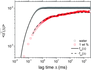 |
| | Fig. 17 Comparison of the time averaged MSD  from 10 individual trajectories for beads of d = 0.96 μm diameter in 1 weight% worm-like micellar solution compared to the control data in pure water.179 Two different fitting curves to the results are depicted: the full solid line represents the exponential relaxation pattern fex(Δ) = 2〈x2〉th(1 − C1e−C2Δ), while the dashed line represents the power-law relaxation behaviour fpo(Δ) = 2〈x2〉th(1 − C3/ΔC4), where Ci are fit parameters. For the data shown here the arbitrary units on the ordinate are converted to nm2 by multiplication with ≈8 × 10³ [179]. from 10 individual trajectories for beads of d = 0.96 μm diameter in 1 weight% worm-like micellar solution compared to the control data in pure water.179 Two different fitting curves to the results are depicted: the full solid line represents the exponential relaxation pattern fex(Δ) = 2〈x2〉th(1 − C1e−C2Δ), while the dashed line represents the power-law relaxation behaviour fpo(Δ) = 2〈x2〉th(1 − C3/ΔC4), where Ci are fit parameters. For the data shown here the arbitrary units on the ordinate are converted to nm2 by multiplication with ≈8 × 10³ [179]. | |
What about ageing, the dependence of some physical observable on the time span ta between initial preparation of the system at t = 0 and start of the measurement (see Fig. 10)? For regular Brownian motion physical observables are independent of the ageing time ta. In the following cases for the FBM/FLE models, however, we find transient ageing. For both FBM and FLE motion the time averaged MSD splits into two additive terms,185
| |
 | (73) |
The stationary term
fst depends solely on the lag time
Δ, while the ageing term
fage is an explicit function of
t and
ta. As long as the initial velocity distribution is not thermal,
fage ≃ 1/
t for long
t. For free FLE motion at sufficiently long
Δ, the stationary term is subdiffusive,
fst ≃
Δ2−α. When additionally we are in the strong ageing regime
ta ≫
t, the scaling
is derived.
185 For confined FLE motion, the ageing term now features the power-law dependence,
185For confined FBM, however, the ageing term decays exponentially,
185| | |
fage ∼ x02exp(−2kta).
| (76) |
Thus, the ageing behaviour for FBM is negligible, while for strongly aged FLE motion the transient ageing may be observable under specific conditions.
5 Scaled Brownian motion
A popular model for the description of anomalous diffusion is that of scaled Brownian motion (SBM), which is based on the time-dependent diffusivity K(t).186–188 The associated Langevin equation with the white Gaussian noise ξ(t) of unit intensity, 〈ξ(t)ξ(t′)〉 = δ(t−t′), and zero mean then becomes| |
 | (77) |
For the power-law formof the diffusion coefficient the MSD of the process is given by eqn (8) with Kα = Γ(1 + α)Kα*. Note that while the physical dimension of K(t) is cm2 s−1, that of the constant Kα* is cm2 s−α. In SBM the scaling exponent is allowed to vary in the range 0 < α < 2, so that the process describes subdiffusion as well as sub-ballistic superdiffusion.
The associated time averaged MSD can be calculated exactly, yielding188,189
| |
 | (79) |
In the limit
Δ ≪
t, we obtain the linear lag time dependence
189,190| |
 | (80) |
familiar from subdiffusive CTRW processes,
eqn (20). However,
expression (80) for SBM is valid in the whole range 0 <
α < 2. When the lag time
Δ approaches the measurement time
t, the limiting form
189| |
 | (81) |
describes a cusp at around
Δ =
t: as shown in
Fig. 18 the time averaged MSD
(81) converges to the value of the MSD 〈
x2(
t)〉. However, while the disparity

between the MSD and its time averaged analogue renders SBM weakly non-ergodic in the sense defined above, the amplitude scatter of

around the trajectory-to-trajectory average

measured in terms of the dimensionless variable
ξ is approximately of Gaussian form with a relatively narrow width. For sufficiently long trajectories, that is, the randomness in single trajectories of SBM is deterministically decreased with time and the process becomes practically reproducible.
189 SBM therefore belongs to a non-ergodicity class, that is fundamentally different from subdiffusive CTRW, for which the randomness of time averages is present no matter how long the process is followed.
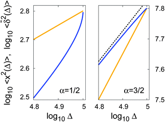 |
| | Fig. 18 Convergence of the time averaged MSD  (blue line) to the MSD 〈x2(t)〉 (orange line) when the lag time Δ approaches the process time t = 105.189 (blue line) to the MSD 〈x2(t)〉 (orange line) when the lag time Δ approaches the process time t = 105.189 | |
Equipping the Langevin eqn (77) for SBM with an additional external potential force F(x), one can derive the associated Fokker–Planck equation. For the special case of a confining harmonic potential V(x) = ½mω2x2 we find189
| |
 | (82) |
where
![[small omega, Greek, macron]](https://www.rsc.org/images/entities/i_char_e0da.gif)
=
ω2/
η includes the friction coefficient
η of dimension s
−1. In the limit of unconfined motion,
ω = 0, the resulting dynamic equation was used by Batchelor
191 to describe the relative diffusion in turbulence as a complementary approach to Richardson's mentioned above (see also Section 6). The force-free propagator encoded by
eqn (82) is exactly that of free FBM,
eqn (56), despite the fundamental difference between the two processes. However, in the presence of the confinement,
ω > 0, we obtain the MSD
| |
〈x2(t)〉 = 2Kα*tαe−2![[small omega, Greek, macron]](https://www.rsc.org/images/entities/i_char_e0da.gif) tM(α,1 + α,2 tM(α,1 + α,2![[small omega, Greek, macron]](https://www.rsc.org/images/entities/i_char_e0da.gif) t) t)
| (83) |
in terms of the Kummer function
M(
a,
b,
z).
192 The limiting behaviour at short times
t ≪ 1/
![[small omega, Greek, macron]](https://www.rsc.org/images/entities/i_char_e0da.gif)
is that of free anomalous diffusion, 〈
x2(
t)〉 = 2
Kα*
tα,
i.e., when the particle starts in the vertex of the potential it initially moves force-free. At long times, we observe that the motion does not become stationary but the MSD exhibits the scaling law
189| |
 | (84) |
The motion is thus influenced by the effective strength
ω of the potential. However, as the diffusion coefficient is explicitly time dependent, this implies that the system is characterised by a time dependent temperature, see also the discussion of Fuliński.
188 Alternatively, one could view this as an effect of a time dependent mobility. Clearly this corresponds to a far from thermal equilibrium state.
For its interesting behaviour, we mention the associated time averaged MSD in the harmonic confinement. In the limit Δ ≪ t we find the result189
| |
 | (85) |
where we observe an apparent plateau at
Δ ≫ 1/
![[small omega, Greek, macron]](https://www.rsc.org/images/entities/i_char_e0da.gif)
,
| |
 | (86) |
as demonstrated in
Fig. 19, in which we compare the full analytic solution
(83) for the MSD and the exact form for the time averaged MSD with results from simulations. In a way, the behaviour is opposite to that of subdiffusive CTRWs, for which we observe the thermal plateau for the MSD and a continuing power-law growth for the time averaged MSD,
45 confirmed by experiment.
68 Experiments observing the apparent plateau
(86) for the time averaged MSD of SBM may misinterpret this for a sign of confinement, contradicting the result
(83).
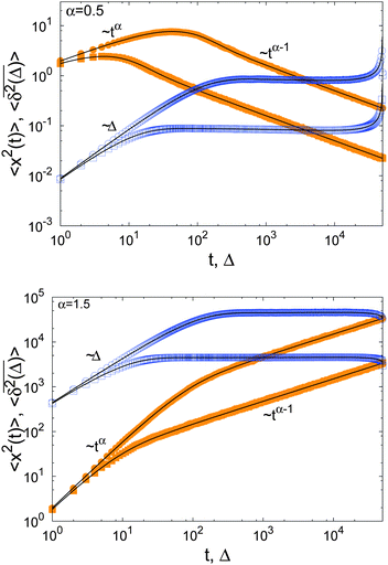 |
| | Fig. 19 MSD 〈x2(t)〉 (orange symbols) and time averaged MSD  (blue symbols) of SBM with α = 0.5 (top) and α = 1.5 (bottom). In each case we consider the potential strengths ω2 = 0.01 (circles) and ω2 = 0.1 (squares). The full lines represent eqn (83) and the numerical evaluation of the exact results for the time averaged MSD.189 The convergence of the corresponding ensemble and time averages at Δ = t = 105 can be shown numerically, in analogy to Fig. 18 for the unconfined motion. (blue symbols) of SBM with α = 0.5 (top) and α = 1.5 (bottom). In each case we consider the potential strengths ω2 = 0.01 (circles) and ω2 = 0.1 (squares). The full lines represent eqn (83) and the numerical evaluation of the exact results for the time averaged MSD.189 The convergence of the corresponding ensemble and time averages at Δ = t = 105 can be shown numerically, in analogy to Fig. 18 for the unconfined motion. | |
In view of these results SBM represents a very simple model for sub- and superdiffusive anomalous diffusion. However, its physicality is somewhat questionable for most experimental settings, in which the system is connected to a heat bath, or when the system is stationary. Its non-ergodic properties are certainly interesting, and may be used to model active processes in the superdiffusive range 1 < α < 2. SBM-type dynamics in fact occurs in free granular gases.289
6 Heterogeneous diffusion processes
Single particle tracking experiments usually employ relatively large tracers. The above mentioned granules and artificial tracers are all in the range of several hundreds of nanometres in size.48–50,68,69,179,193,194 Considerably smaller tracer proteins were recently employed to sample much larger subvolumes of living cells, producing cell-wide mobility maps. The results show significant and systematic variations in the position-dependent cytoplasmic diffusivity K(x) with a growing distance from the nucleus.195 Similar approaches using space-dependent diffusivities are routinely used in various fields, for instance, in the mathematical modelling of tracer dispersion in subsurface hydrology.196 We also recall Richardson's approach to the description of his measurements of the relative dispersion of two tracer particles in a turbulent flow, in terms of a diffusivity depending on the relative tracer position,26 mentioned in the Introduction.
Diffusion processes with position-dependent diffusivity, K(x), are described by a simple Markovian Langevin equation with multiplicative noise197
| |
 | (87) |
where
ξ(
t) represents white Gaussian noise. In the Stratonovich sense, the diffusion equation for this
heterogeneous diffusion process (HDP) has the symmetric form
| |
 | (88) |
A diffusing particle tends to accumulate in regions of low diffusivity. The HDP is fundamentally different from the CTRW approach: standard CTRWs are running off in an annealed environment and thus constitute renewal processes. HDPs represent a deterministic (in contrast to random) quenched environment. The particle, that is, has the same diffusivity
K(
x) each time it returns to the point
x. Interestingly, despite the different nature of HDPs they share some common features such as weak ergodicity breaking with renewal CTRW processes. Even when the space dependence of the diffusivity becomes annealed, many of these effects are preserved.
198
Let us first consider the power-law forms
| |
 | (89) |
for the diffusivity. The amplitude
K0 has physical dimension cm
2−β s
−1. The offset
xoff in
eqn (89) is introduced to avoid either divergencies of
K(
x) (
β < 0) or stalling (
β > 0) of the particle around
x = 0 in the simulations. In the analytical calculations we use the bare scaling form
K(
x) ∼
K0|
x|
β. The HDP based on the diffusivity
(89) and
δ-initial condition for the PDF at the origin has the MSD
197| |
 | (90) |
shown in
Fig. 20. It is thus of the generic power-law form
(8) with the anomalous diffusion exponent
α given in terms of the scaling exponent
β from
eqn (89) as
197| |
 | (91) |
such that we observe superdiffusion in the range 2 >
β > 0 and subdiffusion for
β < 0. We note that when
β approaches the critical value
β = 2, the anomalous diffusion exponent
α diverges. In that case the MSD assumes an exponential time dependence. The PDF of the HDP with power-law diffusivity
(89) is given by the exponential
197| |
 | (92) |
In the subdiffusive range,
β < 0, this PDF is of compressed Gaussian shape and exhibits a dip to zero at the origin, that is, it is bimodal. For superdiffusion with 2 >
β > 0, the PDF is a stretched Gaussian and has a non-differentiable cusp at
x = 0. This is opposite to the behaviour observed for subdiffusive and superdiffusive fractional diffusion equations.
42,199,200
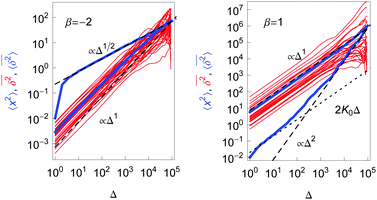 |
| | Fig. 20 Ensemble and time averaged MSDs for sub- and superdiffusive HDP processes with power-law diffusivity (89), for t = 105, and K0 = 0.01. Note that in the simulations, to avoid divergence (subdiffusion) or stalling (superdiffusion) at x = 0, we, respectively, use the forms K(x) = K0/(x2 + 1) and K(x) = K0(|x| + 1). Thin red lines represent individual traces  , thick blue lines refer to the MSD 〈x2(t)〉 and the trajectory average , thick blue lines refer to the MSD 〈x2(t)〉 and the trajectory average  . The expected results (90) and (93) are shown by dashed lines. . The expected results (90) and (93) are shown by dashed lines. | |
For the HDP with the diffusion coefficient (89) we obtain the weakly non-ergodic behaviour197
| |
 | (93) |
Fig. 20 shows the MSD
(8) and the mean time averaged MSD
(93) for a sub- and superdiffusive case. The linear scaling of

is nicely fulfilled, and individual realisations

show pronounced amplitude scatter around this mean. The initial deviation of 〈
x2(
Δ)〉 from the expected behaviour is due to the offset
xoff used in the simulations.
197 The fluctuations of

around the mean

can be fitted by a Gamma distribution for both sub- and superdiffusive HDPs.
197 In contrast to subdiffusive CTRW processes the amplitude scatter distribution
ϕ(
ξ) decays to zero at
ξ = 0, that is, the process never leads to complete stalling of the diffusing particles during the observation time window. Concurrently, the ageing behaviour of HDPs with power-law form of
K(
x) was numerically shown to be in good agreement with the form
(30) of the ageing depression of the CTRW approach.
201 From a data analysis point of view the similar behaviour of various quantities requires some care not to confuse HDPs from CTRW processes.
We note that different forms for the position dependent diffusivity K(x) such as an exponential and logarithmic dependence were studied in ref. 202. The exponential case with K(x) = (K0/2)exp(−2x/x*), where x* sets the length scale, leads to the MSD202
| |
 | (94) |
which belongs to the range of ultraslow processes discussed earlier. The associated time averaged MSD becomes
202| |
 | (95) |
and exhibits an interesting square root scaling in the lag time
Δ for initially highly mobile particles, with initial position
x0 on the negative semi-axis. For intermediate
x0, however, a profound splitting of the tracer populations is observed, exhibiting
Δ1/2 and
Δ1 scaling forms of the time averaged MSD, respectively, for highly mobile and rather trapped fractions of particles in the ensemble. This fact is reminiscent of the population splitting effect observed for CTRW processes, Section 2.1. For more details see
ref. 202. The fluctuations in the HDP model were analysed in more detail in
ref. 197, and a two-dimensional analysis paraphrasing the mobility experiments in living cells in
ref. 195 was presented recently.
203
In Fig. 21 we demonstrate how under confinement the ensemble and time averaged MSDs converge to the plateau value
| |
 | (96) |
where
ν ≃ 0.6 and 2
L is the length of the interval with reflecting boundaries.
201 The convergence to the plateau for both ensemble and time averaged MSDs (with the aforementioned factor of two for the time average) sets the HDP process apart from the subdiffusive CTRW, in which no long time plateau occurs for

.
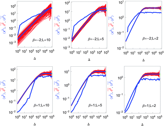 |
| | Fig. 21 MSD 〈x2(t)〉 (thick blue curves), time averaged MSDs  (thin red curves), and trajectory average (thin red curves), and trajectory average  (thick blue curves) for confined HDPs with power-law diffusivity (89) and different exponents β.201 All curves converge to the plateau value (96). For each exponent β we show N = 300 time averaged traces of length t = 105 in the interval {−L,L}. (thick blue curves) for confined HDPs with power-law diffusivity (89) and different exponents β.201 All curves converge to the plateau value (96). For each exponent β we show N = 300 time averaged traces of length t = 105 in the interval {−L,L}. | |
Finally, Fig. 22 shows the result for a typical trajectory in the recent study of ref. 198, in which a random walker travels on a landscape with randomly switching local diffusivity. As can be seen from the graph, on finer scales the motion appears to be more like normal diffusion, due to the broad distribution of K(x) magnitudes, on a coarser resolution the trajectory appears to be similar to that of a subdiffusive CTRW with a diverging characteristic time scale shown in Fig. 6. It will be interesting to compare these results to the behaviour of stochastic HDPs in annealed and quenched environments.204
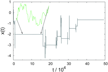 |
| | Fig. 22 Trajectory in the heterogeneous diffusivity domain model of ref. 198. While on short scales the process appears to be Brownian (inset) on the larger scale distinct stalling events are reminiscent of scale-free CTRW dynamics. Data for the figure courtesy John Lapeyre. | |
7 Fractals
Finally we come to the third major model for anomalous diffusion, namely, the transport on a fractal support. Like fractional Brownian motion and Lévy flights, fractals were popularised by Mandelbrot, in whose book The fractal geometry of nature he came up with the epitomised phrase Clouds are not spheres, mountains are not cones, coastlines are not circles, and bark is not smooth, nor does lightning travel in a straight line.124 Instead, Mandelbrot argues that many natural phenomena are statistical fractals, i.e., objects which, in a statistical sense, do not have a scale and thus one cannot judge at what resolution a picture of the object was taken. Or, in other words, their length (or area, etc.) depends on the applied scale in a measurement, as in the celebrated coastline of the Britain paradox: with a smaller yardstick finer details can be measured and the length of the coastline is larger than when we apply a larger yardstick. Mandelbrot accredits the discovery of this effect to Lewis Fry Richardson.205,206
We distinguish mathematical fractals with their strict building rules and exact self-similarity from statistical fractals, for which self-similarity is present only in a certain average sense. Let us briefly address these two concepts. First, mathematical fractals are constructed by iteration. For instance, see the Sierpińsi gasket in Fig. 23. An equilateral triangle is divided into four equilateral triangles and the central one removed. This subdivision rule is repeated, ideally an infinite amount of times. From the iteration scheme: scale the original triangle down by a factor of 2 and keep three of the resulting four objects, we obtain the similarity dimension log![[thin space (1/6-em)]](https://www.rsc.org/images/entities/char_2009.gif) 3/log
3/log![[thin space (1/6-em)]](https://www.rsc.org/images/entities/char_2009.gif) 2 ≃ 1.585, which gives the same result as the formal Hausdorff approach.124,207 We would obtain the same result if we had started by arranging three copies of the original triangle into an object with twice the original edge length. The Sierpińsi gasket is more space filling than a line but does not fully fill an area. In particular, we see that the generated object contains empty triangles on all scales. To come from one given sector to another, a random walker on such a geometry needs to first locate and then traverse narrow causeways, as sketched in Fig. 24. This considerably slows down the particle propagation in the embedding space.
2 ≃ 1.585, which gives the same result as the formal Hausdorff approach.124,207 We would obtain the same result if we had started by arranging three copies of the original triangle into an object with twice the original edge length. The Sierpińsi gasket is more space filling than a line but does not fully fill an area. In particular, we see that the generated object contains empty triangles on all scales. To come from one given sector to another, a random walker on such a geometry needs to first locate and then traverse narrow causeways, as sketched in Fig. 24. This considerably slows down the particle propagation in the embedding space.
 |
| | Fig. 23 Sierpińsi gasket. An equilateral triangle is constructed iteratively such that the edges of three congruent triangles make up the edges of a triangle twice their size. The centre of this larger triangle remains empty. Here we show the fourth generation of the Sierpińsi gasket. | |
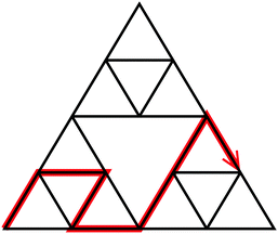 |
| | Fig. 24 A random walk on part of a Sierpińsi gasket. Each time the walker wants to reach a sector of the gasket across one of the larger holes, it needs to traverse a narrow causeway. | |
As said, natural objects are not exact mathematical fractals. However, for example, the coastlines of Britain or Norway are statistical fractals: while their shape does not repeat exactly on a smaller scale, their overall length fulfils a scaling law L(ε) ≃ ε1−df, where ε is the length of the yard stick applied to measure the coastline.124,149,208,209 If the coastline were a perfect line with df = 1, its length L would be independent of the length ε of the yard stick (resolution) applied for the measurement. However, within a certain upper length scale—of the order of the extension of the country—and a lower length scale—e.g., the finest features appearing on a map—the fractal dimension of coastlines typically differs from unity. Thus, while the South African coastline with df = 1.02 is almost a perfect line, the West coast of Britain has df = 1.25, and is thus significantly more ramified. For finer measurement resolutions (shorter yard stick length ε) the measured length increases, while coarser measurements (longer yard stick length ε) lead to shorter apparent L. For general fractals with a fractal dimension df embedded in a d-dimensional space, it is often useful to think in terms of the mass of the fractal object, which, on average, grows like M(R) ≃ Rdf as a function of the radius R. As by necessity df < d, the mass density therefore shrinks with R as Rdf−d, as fractals are characterised by ‘holes’ on all scales (compare the Sierpińsi gasket in Fig. 23).
An important approach to the description of porous or crowded media is the percolation model. In site percolation each point on a lattice is occupied with probability p and remains empty with probability 1 − p. At the critical occupation probability p = pc (pc ≃ 0.59… in two210 and pc ≃ 0.31… in three211 dimensions for a square and cubic lattice, respectively) the correlation length of the system diverges and an infinite cluster is formed. The percolation cluster then has a fractal dimension df = 91/48 ≃ 1.896… in two212 and df ≃ 2.52… in three dimensions.213 A random walker placed on the fractal, incipient infinite cluster allowed to move between nearest neighbour occupied sites performs anomalous diffusion with an anomalous diffusion exponent α = 2/dw related to the walk exponent dw, which is larger than df.214,215 According to the Alexander Orbach conjecture dw = ![[/]](https://www.rsc.org/images/entities/char_e0ee.gif) df,215 which is close to experimentally observed values, compare ref. 216. Note that when the averaged motion of random walkers placed on all clusters, a different scaling exponent characterises the MSD, for more details see ref. 217.
df,215 which is close to experimentally observed values, compare ref. 216. Note that when the averaged motion of random walkers placed on all clusters, a different scaling exponent characterises the MSD, for more details see ref. 217.
Fig. 25 shows the critical percolation cluster on a square lattice used for random walk simulations in ref. 218. The results for both the two-dimensional MSD 〈r2(t)〉 and time averaged MSD  for the motion on the infinite cluster are shown in Fig. 26. Both overlap perfectly, corroborating the ergodicity of this anomalous diffusion process. The straight line in Fig. 26 indicates the expected slope to guide the eye. In ref. 219, the non-Gaussian nature of the diffusion on the critical percolation cluster is analysed. Fractal percolation clusters are often used for simulations of free diffusive processes220 as well as facilitated diffusion processes221 in the crowded cytoplasm of living biological cells. A fractal support was also diagnosed to be superimposed onto the subdiffusive CTRW motion for the diffusion of potassium channels in the plasma membrane of living human cells in ref. 50. It is important to note that when we consider the motion on all clusters the motion is a forteriori no longer ergodic: a walker moving on a finite, disconnected cluster cannot explore the entire phase space.217
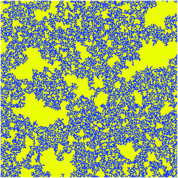 |
| | Fig. 25 Percolation cluster at criticality on a 250 × 250 square lattice. Occupied sites appear blue. Data provided by Y. Meroz, corresponding to those used in ref. 218. | |
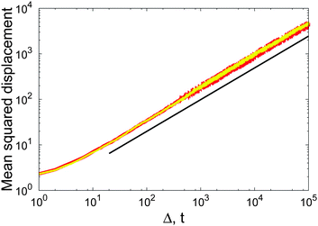 |
| | Fig. 26 MSD (thicker red curve) and time averaged MSD (thinner yellow curve) of a random walk on the infinite critical percolation cluster shown in Fig. 25. Both MSD and time averaged MSD perfectly overlap, i.e., diffusion on a fractal is stationary and ergodic. The straight black line shows the expected slope α = 0.697 to guide the eye. Data provided by Y. Meroz, corresponding to those used in ref. 218. | |
While the increments of random walk processes on fractal structures are stationary31 and the infinite percolation cluster simulations of ref. 218 indicate that diffusion on fractals is ergodic, this point needs further investigation, in particular, for different types of fractals; compare also the discussion in ref. 222. A second open question is what happens in the presence of a topological bias, for instance, a bias away from the backbones208 of a diffusion cluster. In that case at least transient non-ergodicity would be expected.
8 Strong anomalous diffusion and infinite densities
So far we have focused our attention on the ensemble averaged MSD 〈x2(t)〉 and the corresponding time average  . More generally, one may characterise stochastic processes by their fractional moments 〈|x(t)|q〉 with q ≥ 0. Strong anomalous diffusion deals with processes, which in the long time limit satisfy223where ν(q) is not a constant. For Brownian motion ν(q) = 1/2 and for FBM ν(q) = α/2 so that these processes do not exhibit strong anomalous diffusion. For unbiased Gaussian processes like FBM the MSD characterises the width of the PDF P(x,t) when the particles start at the origin x = 0. For this reason, from the starting days of the Gaussian central limit theorem the variance of the stochastic process has attracted special attention. Experimentally, information on 〈|x(t)|q〉 is used to support or dispute the Gaussian nature of an underlying diffusion process or, more generally, the mono-scaling assumption of a set of data (see below). When dealing with complex transport of particles, for example tracer particles in living cells when periods of active motion contribute to the motion, the spectrum of exponents qν(q) may in fact exhibit non-Gaussian and strong-anomalous statistics.224
Recent experimental studies on the active transport of polystyrene beads in living cells exhibit a particular type of strong anomalous diffusion. The data analysis exhibits piecewise linear behaviour with
| |
 | (98) |
with the positive constants
qc,
μ,
a, and
b. Such a behaviour is sometimes called bi-fractal scaling, as the simplest case of multi-fractal behaviour. More importantly this bi-linear behaviour is widespread and found in many models of non-linear dynamics,
223,225–229 transport in optical lattices,
230,231 models of transport in disordered Lévy glasses,
232–234 and other stochastic models.
88,235,236 The parameters
qc,
μ,
a, and
b are non-universal and hence give specific information on the underlying model or process. As emphasised by Vulpiani and coworkers
223 strong anomalous diffusion implies the breakdown of mono-scaling theories which predict
P(
x,
t) ∼
t−νf(
x/
tν) in terms of a scaling function
f(·). For example, FBM, FLE, sub-diffusive decoupled CTRW, and fractional diffusion equations,
42,56 do not predict the piecewise bi-linear scaling
(98) of the moments, in other words these popular stochastic models considered above cannot describe the active transport found in
ref. 224. In experiments
a ≃ 0.8 (see discussion below).
Roughly speaking, the piecewise linear scaling of the spectrum qν(q) implies that lower order moments q < qc still follow a diffusive, possibly anomalous process if μ ≠ 1, while the linear increase of the spectrum qν(q) ∼ q for q ≫ 1 implies a ballistic scaling, since if x scales like t, 〈|x|q〉 scales with tq. This implies that the process is actually a mixture of both diffusive process x ∝ tμ and ballistic element x ∝ t, and hence characterising the process as an anomalous diffusion process is in some sense misleading. In particular, we should not universally accept the special role of the second moment, beyond the fact that it indicates certain deviations from normal behaviour. A typical situation occurs when P(x,t) for small x scales diffusively (ν = 1/2), however, for certain large x the scaling becomes ballistic (ν = 1). Here we focus on one stochastic model of strong anomalous diffusion, the Lévy walk model mentioned in Section 3.5. For more details on the mathematical treatment of the following, see ref. 237.
Lévy walks represent a widely applicable model describing superdiffusion.51,81,238–244 In its simplest one dimensional version, a particle starts at the origin at time t = 0, and travels with velocity v1, drawn from the PDF F(v). The duration of the travelling event is τ1 which is drawn from the PDF ψ(τ). The position of the particle at time τ1 is x = v1τ1. The process is then renewed, until time t is reached: a new velocity v2 and waiting time τ2 are independently drawn from F(v) and ψ(τ), and this process is repeated. The position of the particle is then simply  . If the PDF ψ(τ) of the flight duration is exponential and the velocity distribution Gaussian with zero mean, we recover the famous Drude model.245 Ergodic properties of Lévy walks were analysed in ref. 136–138, see also Section 2.5.
We assume that the velocity PDF is symmetric—F(v) = F(−v), such that 〈v〉 = 0—and that all moments of F(v) are finite, for instance, a Gaussian PDF. The main ingredients of the stochastic model are the power-law distributed waiting times (14). These can be justified from first principles models or from observations, at least in some systems, compare the discussions in ref. 39, 51 and 241. We here limit our discussion to the case 1 < α < 2 which in turn implies that the average sojourn time 〈τ〉 is finite, however, its variance diverges. Rather generally, it is easy to understand that the MSD is bounded by 〈x2(t)〉 < 〈v2〉t2. Roughly speaking, the ith jump in the process is given by δxi = viτi, and due to the assumed power-law PDF of waiting times the PDF of this increment is a symmetric distribution (due to the symmetry of the distribution of v) with long tails
The typical number of jumps in the process is
N ≃
t/〈
τ〉. Hence a hand-waving argument yields the PDF of the position of the particle using the generalised central limit theorem. Namely,

with the variance of
δxi being infinite, such that we expect that the PDF of particles is given by (in dimensionless units)
| |
 | (100) |
here
Lα,0(
x) is the symmetric Lévy distribution, whose Fourier pair is exp(−|
k|
α), such that the case
α = 2 corresponds to a Gaussian process. Taken seriously, this central limit theorem implies
| |
 | (101) |
These hand-waving arguments provide the correct scaling of the lower order moments, however, the results for higher order moments, including the second moment, are obviously wrong: the particle cannot travel faster than ballistic motion.
|||||| Our argument is flawed since we have neglected the correlation between the jump sized and time in the problem. A more precise mathematical analysis leads to the result
237| |
 | (102) |
In terms of the parameters introduced in
eqn (98), we thus identify
μ = 1/
α,
qc =
α,
a = 1, and
b =
α − 1. We see that the process exhibits strong anomalous diffusion,
223,237,246 the MSD exhibits enhanced diffusion 〈
x2〉 ∼
t3−α which is faster than normal but slower than ballistic, 1 < 3 −
α < 2. The lower order moments
q <
α exhibit Lévy scaling,
i.e., what we call anomalous diffusive scaling. In contrast, the higher order moments are ballistic in the sense that if
q ≫ 1 we have
qν(
q) =
q + 1 −
α →
q, the ballistic scaling. The power law tail of the Lévy PDF is cut off at
x ≃
t since particles cannot travel faster than the typical velocity permits, compare
ref. 133. This Lévy walk picture thus cures the divergence of the moments beyond
q =
α of the original Lévy flight.
The fact that experimentally224 one finds a = 0.8 and therefore qν(q) ∼ 0.8q and not qν(q) ∼q shows that purely ballistic motion between turning points is not a sufficient model to describe the measured behaviour. At least on the stochastic level this may imply that non-linear relations between jump size and waiting times are important. The experimental finding of non-ballistic scaling of large-q moments (in experiment the largest q was 8) is an indication for the insights one can achieve by analysis of time dependence of moments.
8.1 Infinite densities
At the heart of the mathematical theory of diffusive phenomena stand the Gauss and Lévy central limit theorems. A piecewise linear scaling of the moments in our example implies that the Lévy central limit theorem is a valid approximation at the central part of the PDF of particles but not in the tails. The fact that we have only two scaling behaviours of the moments may suggest that in addition to the central limit theorem there exists another general method to describe the fluctuations. Such a theory was recently obtained237 and the problem related to infinite densities. These are a class of non-normalised densities that have only recently attracted attention from physicists.
According to eqn (102) the moments 〈|x|q〉 with q < α are given by the Lévy density. The higher order moments with q > α are also calculated from a density denoted ![[scr I, script letter I]](https://www.rsc.org/images/entities/char_e143.gif) D(·),237
D(·),237
| |
 | (103) |
![[scr I, script letter I]](https://www.rsc.org/images/entities/char_e143.gif) D
D(

) is called an infinite density, in the sense that it yields the moments 〈|
x|
q〉 with
q >
α but at the same time is not normalised,
| |
 | (104) |
(see below for the physical meaning of

). The density
![[scr I, script letter I]](https://www.rsc.org/images/entities/char_e143.gif) D
D(·) is complimentary to the Lévy density. The infinite respective Lévy densities fail to provide statistical information on the moments
q <
α or
q >
α, but are useful for
q >
α respective
q <
α. The identity of the observable of interest is thus crucial,
e.g., 〈
x2(
t)〉
versus 〈|
x(
t)|〉, in the sense that not only they yield different scaling behaviours with time (strong anomalous diffusion) but they are calculated from two different scaling functions. More specifically, the infinite density has the small

behaviour
237which is non-integrable and hence non-normalisable. Note that this non-integrability is cured when we calculate, for example, the second moment, since
 2
2 −1−α
−1−α is integrable close to

→0. This is the reason why this function can give information on the higher order moments
q >
α.
However, is the infinite density merely a mathematical construction with which we obtain statistical information on the moments of the process, or does it actually contain information on the particle PDF? Since  at all times, one may wonder why a non-normalised solution emerges? The infinite density and the density P(x,t) are related according to237
| |
![[scr I, script letter I]](https://www.rsc.org/images/entities/char_e143.gif) D( D( ) ∼ tαP(x,t) ) ∼ tαP(x,t)
| (106) |
where

is the time averaged velocity. Since

, the integral over the infinite density diverges when
t → ∞. Importantly,
eqn (106) implies that if we plot the density of particles (normalised to unity, with an initial condition at the origin) according to
tαP(
x,
t)
versus x/
t and
t1/αP(
x,
t)
versus x/
t1/α, the data in both cases will collapse onto a master curve. In the first way of plotting this curve will be the infinite density, and thus we can estimate this density from numerical or experimental data. In the second plot we get the well known Lévy density.
237 This dual scaling is obviously related to the bi-linear behaviour of the spectrum
qν(
q). Since the latter is very common we believe that infinite densities also have some general validity. In mathematics, infinite densities, briefly discussed here, are a subject of research for many years, in the context of infinite ergodic theory.
247–249 This branch of pure mathematics is in fact related to the phenomenon of weak ergodicity breaking discussed here.
250
For the Lévy walk model one can obtain explicit formulae for the infinite density in terms of the parameters of the model.237 It was shown that this density depends on three measurables: F(v), α, and the anomalous diffusion constant which characterises the width of the Lévy density.237 In that sense the infinite density yields statistical information not contained in the central limit theorem, namely it contains more fingerprints of the underlying process: the velocity distribution (which can, in principle, be measured independently). The small  behaviour of
 ![[scr I, script letter I]](https://www.rsc.org/images/entities/char_e143.gif) D(
D( ) is not sensitive to the shape of F(v) (provided it is symmetric) and in that sense it is universal. For example, for a Gaussian F(v), the infinite density is plotted in Fig. 27. We believe that further work on infinite densities is required since only recently these have attracted some attention in statistical physics83,230,251–254
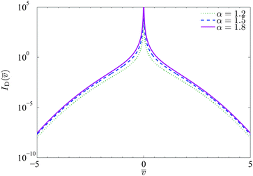 |
| | Fig. 27 Infinite density for a Gaussian velocity distribution F(v). Notice the divergence of the density at the origin. This divergence is non-integrable, hence these functions are non-normalisable. Still, they describe the statistical properties of physical particles.237 | |
9 Measurables
Normal and anomalous diffusion are key to many biological signalling processes and a vast number of biochemical reactions in cells, or to the spreading dynamics in inanimate complex systems. To be able to analyse diffusion measurements in a physical meaningful way and to make predictions for secondary processes such as reaction rates or signalling cascades, it is absolutely necessary to know the exact nature of the stochastic process driving the particle motion. For instance, the first passage behaviour is vastly different between the processes reviewed here. In this section we describe some experimentally relevant observables whose complementary character enables one to attain a fair degree of certainty that a given set of data is based on a concrete stochastic process. Analyses based on the application of different measures are, for instance, presented in ref. 44, 50, 68, 69, 175, 176 and 255–260. As demonstrated in the literature,50,68,69,72 we note that there is a priori no good reason to assume that in a complex system one of the above processes is sufficient to adequately describe all the observed dynamic features: sometimes it is necessary to combine at least two of the processes, which may influence the particle motion simultaneously or at different time scales. When passive diffusion is combined with intermittent active motion additional challenges to the data analysis arise.261
MSD
The MSD is unarguably the most common way to analyse stochastic data. Depending on the kind of measurement the quantity to evaluate is the MSD 〈x2(t)〉 or the time averaged MSD  . The latter is the typical approach to the analysis of the time series obtained from single particle tracking. If the time averaged MSD exhibits anomalous scaling of the form
  and
and  we are dealing with an (asymptotically) ergodic process, and when we want to use the data to identify the underlying stochastic process we can even eliminate CTRW motion and diffusion processes with time or space dependent diffusivity as sole contributions. To be more specific, additional complementary measures need to be evaluated.
Scatter of time averages
The statistics of the scatter of the amplitude  of the time averaged MSD for a set of individual trajectories at a given lag time Δ is a useful indicator for the classification of the anomalous diffusion process. We quantify this scatter by the distribution ϕ(ξ) of the dimensionless amplitude
  and by its variance, the ergodicity breaking parameter EB = 〈ξ2〉 − 〈ξ〉2 introduced earlier. As a general trend the fluctuations increase for any type of motion when the lag time is taken too large in comparison to the measurement time t. We note that due to the very definition (6) of the time averaged MSD the plateau value observed for some of the processes under confinement is twice the value of the MSD. When the lag time approaches t, the time averaged MSD
  shows a cusp to the thermal value 〈x2〉th, as shown explicitly for the SBM model in ref. 189.
For Brownian motion the PDF ϕ(ξ) converges to the sharp form ϕ(ξ) → δ(ξ − 1) around the ergodic value ξ = 1 in the long time limit t → ∞. At finite t this δ-peak broadens. Individual trajectories exhibit erratic fluctuations of  as Δ → t. The ergodicity breaking parameter tends to zero with the ratio Δ/t in the form EB ∼ Δ/t.
For subdiffusive CTRW motion the trajectory-to-trajectory fluctuations are asymptotic, that is, the ergodicity breaking parameter has the finite limiting value (25) varying with α between unity and zero. As in this process the fluctuations are statistically given by the number of jumps performed during its time evolution,73 the PDF ϕ(ξ) remains unchanged when the process becomes confined. The distribution ϕ(ξ) has a finite value at ξ = 0 for any given Δ, a strong characteristic of the weakly non-ergodic CTRW motion. For aged CTRW processes ϕ(ξ) has a discrete immobile contribution proportional to δ(ξ) and a continuum part whose distribution is qualitatively similar to the non-aged process, albeit there occurs a redistribution of this continuous part to larger ξ values.73 The PDF ϕ(ξ) for noisy CTRW processes with superimposed Ornstein–Uhlenbeck or Brownian noise narrows down for increasing noise strength.98 Finally, we note that subdiffusive CTRW processes with a cutoff of the power-law waiting time distribution exhibit an MSD with all features of the process with a diverging waiting time scale roughly up to the cutoff time, however, due to the lack of extreme waiting events the scatter distribution ϕ(ξ) appears to be significantly more ergodic,68 compare also the discussion in ref. 262 and 263.
For FBM and FLE motion the scatter distribution at sufficiently short lag times is Gaussian and becomes somewhat asymmetric but preserves the property ϕ(0) = 0 for larger Δ.158 The ergodicity breaking parameter tends to zero with the ratio Δ/t.156 For the transiently non-ergodic behaviour under confinement see ref. 166 and 179. In general, the scatter distribution and the ergodicity breaking parameter of both processes are relatively similar to those of regular Brownian motion.
SBM was shown to be a weakly non-ergodic process but its ergodicity breaking parameter tends to zero with the ratio Δ/t.189,190 The PDF ϕ(ξ) is approximately bell-shaped albeit wider than for the corresponding FBM with identical anomalous diffusion exponent α.
For HDPs the form of the PDF ϕ(ξ) follows an asymmetric Rayleigh-like or generalised Gamma distribution.197 The width of ϕ(ξ) for HDPs with power-law form (89) grows from the minimal Brownian value attained for the scaling exponent β = 0 of K(x) and diverges at the critical point β → 2. For confined HDPs the width of ϕ(ξ) decreases drastically for all β values, often reaching only a minute scatter. The ergodicity breaking parameter tends to zero as 1/t for fixed Δ.201
We note that in some cases, in lieu of the ergodicity breaking parameter defined above—which represents a sufficient condition for (non-)ergodicity—one uses the parameter  ,138 representing a necessary condition for ergodicity.
First passage time statistics
When sufficient statistics are available one may use the first passage time statistics to distinguish different kinds of anomalous diffusion processes. In single particle tracking experiments the first passage can simply be measured as the moments in time when the tracer passes a certain distance from its original point of release. As shown in ref. 264 the scaling of the mean first passage time obtained from a statistical number of repeats of such an experiment with the distance from the origin may be a good indicator for the underlying diffusion process. Moreover, the PDF of first passage times can be a good indicator, especially for confined systems. While subdiffusive CTRW processes with their scale-free waiting times still exhibit a power-law decay under confinement,42,94 other processes have an exponential form of the first passage PDF. For semi-open intervals, we note that the dependence of the scaling exponent for the first passage PDF on the stochastic process may either be increasing or decreasing**** with the anomalous diffusion exponent α, and could thus also serve as an indicator when α is varied.
Mean maximal excursions and higher order moments
Apart from the regular PDF P(x,t) a stochastic process may be characterised by another, related quantity, the PDF of the maximal excursion. This PDF measures the likelihood that at some time t after its initial release at the origin, the particle has not travelled farther than the distance x.256,265 This distribution may be reconstructed from the measured single particle traces, and then higher order moments calculated from the data. For CTRW and FBM the scaling behaviour of the second moment of the mean maximal excursion as well as the fourth moments are known. It can be shown that the ratios of the regular moments 〈x4〉/〈x2〉2 and the corresponding quantities of the mean maximal excursions obey certain inequalities.256 The behaviour of the other processes with respect to this method remain to be analysed. However, we mention that the method of the mean maximal excursion has a clear advantage over the regular PDF as the mean maximal excursion dynamics is less dispersed and the associated moments therefore more reliable for finite data sets.256
Distribution of local diffusivity
An interesting tool to analyse single particle tracking data is to measure the distribution of the local anomalous diffusion coefficient as a function of the (lag) time from the ratio of the MSD (time averaged MSD) versus the (lag) time to some positive power. These distributions for a weakly non-ergodic process are different according to whether the MSD or the time averaged MSD is evaluated. A detailed discussion for Brownian processes with spatially varying diffusivity and for CTRW processes can be found in ref. 266 and 267. This method still needs to be analysed for the other anomalous stochastic processes considered herein.
Non-Gaussianity measure
Similar to the ergodicity breaking parameter EB, the non-Gaussianity measure G involves higher order moments. In terms of the experimentally relevant time averaged MSD we define the non-Gaussianity as217| |
 | (107) |
in dimension d, where the fourth time averaged moment is defined via| |
 | (108) |
For Brownian motion G = 0, while this parameter deviates from zero for progressively non-Gaussian diffusion. The value of G provides a sensitive measure for the type of diffusion process under consideration. For instance, based on G measurements for diffusion of fluorescent nanobeads in complex crowded fluids, the Gaussian FBM-like process was recently proposed as a suitable mathematical model rather than a CTRW process.268
The p-variation method
The p-variation method is based on the evaluation of the pth power of a partial sum of increments of a given stochastic process.177,269 It was applied as a measure to distinguish the non-Gaussian subdiffusive CTRW from the Gaussian FBM process.177,269 An attractive feature of the p-variation test is its applicability to both unbounded and confined systems, even when based on a single sufficiently long experimental trace. When the recorded time traces are affected by a highly noisy environment, the p-variation test may become inconclusive.98
Velocity auto correlation
The experimentally accessible correlation of increments along some time trace x(t) can be probed in terms of the covariance44| | |
C(ε)ν(τ) = ε−2〈(x(τ + ε) − x(τ))(x(ε) − x(0))〉.
| (109) |
Although it is based on increments of the position rather than on the real velocity of the particle, the quantity (109) is often referred to as the velocity auto-correlation function of the process x(t). For free, unconfined CTRW processes this function drops to zero algebraically as C(ε)ν(τ) ∼ 1 − (τ/ε)α and vanishes at τ > ε due to the independence of successive steps.44 With this property CTRW motion is easily distinguishable from unconfined FBM, the latter being characterised by a crossover to negative values (a signature of the antipersistence) and a power-law recovery back to zero. The autocorrelation can be successfully used to analyse the nature of an anomalous diffusion process.166,197 However, for confined motion also the CTRW process exhibits some form of antipersistence due to the reflections at the boundaries or the rising flanks of the confining potential. In that case the behaviour of the function C(ε)ν(τ) becomes empirically indistinguishable between confined CTRW and FBM.44
10 Discussion and conclusions
Brownian diffusion with its Gaussian propagator has an appealing beauty in its universality. No matter what the exact details of the underlying process are, the limiting behaviour is completely determined by the MSD and its linear growth with time. Concurrently, it is ergodic, so all quantities measured as time averages of sufficiently long single trajectories can be safely interpreted in terms of the readily available theoretical results in terms of ensemble averages. At the same time one could also perceive Brownian diffusion as somewhat too restrictive: many experimental observations are much richer and cannot be explained by the Gaussian propagator emanating from the central limit theorem. We note that while it may be true that apparent anomalous diffusion may in fact be due to transient crossovers of Brownian motion in confined geometries270–274 the opposite may also be true: some diffusion processes failed under Brownian motion may in reality be anomalous.64 One of the reasons may be the weakly non-ergodic behaviour discussed in this review.
Especially since more refined measurement techniques such as space resolved fluorescence recovery after photobleaching measurements and, in particular, high resolution single particle tracking have become available, anomalous diffusion has been widely observed. Most importantly, information beyond the time scaling of the MSD can be extracted from the data. These observations demonstrate that in different systems anomalous diffusion has different diffusive, first passage, and ergodic characteristics. In particular, disparities between ensembles and time averaged observables have been reported. Accommodating the features of anomalous diffusion and non-ergodicity poses the challenge to come up with a pluralistic range of stochastic models for the description of non-Brownian diffusion processes.
We here summarised the state of the art in the study of the properties of the most popular anomalous diffusion processes. In view of their importance in the analysis of experimental or simulations data we paid specific attention to the time and ensemble averaged MSDs. For ergodic processes both quantities are identical for sufficiently long measurements and ensembles. In the opposite case, when time and ensemble averaged MSDs are asymptotically disparate, we speak of a weakly non-ergodic process. The rich range of behaviours is listed in Table 1. In the sense of the ensemble averaged MSD, the considered models span from cubic time scaling down to ultraslow, logarithmic time evolution. Considering the lag time dependence of the time averaged MSD, the variation is much narrower, from quadratic scaling to a square root dependence. In most weakly non-ergodic cases a linear lag time dependence is observed and may be falsely interpreted as normal diffusion.
From a statistical physics point of view the variety of behaviours listed in Table 1 poses a number of questions, in particular, for a classification scheme of anomalous diffusion processes with respect to their (non-)ergodic behaviour and how fundamental mathematical concepts have to be generalised, for instance, the Khinchin theorem.45 Moreover, it is of principle interest whether we can construct new processes, which break the linear lag time scaling of  . At the same time there are still a number of open questions concerning the processes reviewed here, for instance, the exact form of the ergodicity breaking parameter EB beyond the CTRW case. Another question is to come up with additional methods to diagnose the underlying stochastic process from a given, limited set of data from experiments or computer simulations. In particular, Bayesian inference methods are expected to be developed further. The latter should also work well when the observed process in fact represents a blend of different stochastic processes.
It will also be of interest to extend the study of the ergodic behaviour and the features of ageing from the stochastic processes considered here to more specific systems. The latter include, for instance, the Lorentz gas model with its rich behaviour of crossovers and density effects,280 the motion in periodically structured environments such as elastic gels,97 or the folding dynamics of proteins.170,281 Other interesting current questions concern the understanding from a stochastic point of view of Fickian yet non-Gaussian diffusion processes,282–284 compare also the discussion in ref. 285. Finally we mention that similar concepts to those summarised here could be relevant for active transport processes. From a more practical point of view, the discussion of the question as to what extent anomalous diffusion may impact biological function has just begun.32,33,217,221,286–288
Abbreviations and symbols
Symbols used in the text are summarised in Table 2.
| CTRW | Continuous time random walk |
| FBM | Fractional Brownian motion |
| FLE | Fractional Langevin equation |
| HDP | Heterogeneous diffusion process |
| MSD | Mean squared displacement |
| PDF | Probability density function |
| SBM | Scaled Brownian motion |
Acknowledgements
We thank Yasmine Meroz for kindly providing the simulations data for Fig. 25 and 26. We ackowledge discussions with Golan Bel, Olivier Bénichou, Stas Burov, Aleksei Chechkin, Weihua Deng, Sergey Denisov, Daniela Froemberg, Aljaz Godec, Igor Goychuk, Peter Hänggi, Yong He, Joseph Klafter, Diego Krapf, Katja Lindenberg, Eric Lutz, Macin Magdziarz, Lene Oddershede, Gleb Oshanin, Günther Radons, Adi Rebensthok, Johannes Schulz, Igor Sokolov, Matthias Weiss, and Aleksander Weron. RM and JHJ acknowledge financial support from the Academy of Finland through the FiDiPro programme. EB acknoledges financial support from the Israel Science Foundation. AGC acknowledges funding from the Deutsche Forschungsgemeinschaft (grant CH 707/5-1).
References
- A. Einstein, in Investigations on the theory of the Brownian movement, ed. R. Fürth, Dover, New York, NY, 1956 Search PubMed.
- R. Brown, Philos. Mag., 1828, 4, 161 Search PubMed; R. Brown, Ann. Phys. Chem., 1828, 14, 294 CrossRef.
- M. Gouy, J. Phys., 1888, 7, 561 Search PubMed.
- M. von Smoluchowski, Ann. Phys., 1906, 21, 756 CrossRef CAS.
- A. Fick, Ann. Phys., 1855, 170, 59 CrossRef.
- P. Langevin, Acad. Sci., Paris, C. R., 1908, 146, 530 CAS.
- W. T. Coffey and Y. P. Kalmykov, The Langevin equation, World Scientific, Singapore, 2012 Search PubMed.
- M. D. Haw, J. Phys.: Condens. Matter, 2002, 14, 7769 CrossRef CAS.
- J. Perrin, Acad. Sci., Paris, C. R., 1908, 146, 967 CAS; J. Perrin, Ann. Chim. Phys., 1909, 18, 5 Search PubMed.
- T. N. Thiele, Vidensk. Selsk. Skr. 5. Rk., naturvid. og mat. Afd., 1880, 12, 381 Search PubMed.
- L. Bachelier, Annales Scientifiques de l'École Normale Supérieure, 1900, 3, 21 Search PubMed.
- W. Sutherland, Philos. Mag., 1905, 9, 781 CrossRef CAS.
- I. Nordlund, Z. Phys. Chem., 1914, 87, 40 CAS.
- E. Kappler, Ann. Phys., 1931, 11, 233 CrossRef CAS.
- W. E. Moerner and M. Orrit, Science, 1999, 238, 1670 CrossRef.
- M. J. Saxton and K. Jacobsen, Annu. Rev. Biophys. Biomol. Struct., 1997, 26, 373 CrossRef CAS PubMed.
- C. Bräuchle, D. C. Lamb and J. Michaelis, Single Particle Tracking and Single Molecule Energy Transfer, Wiley-VCH, Weinheim, Germany, 2012 Search PubMed.
- X. S. Xie, P. J. Choi, G.-W. Li, N. K. Lee and G. Lia, Annu. Rev. Biophys., 2008, 37, 417 CrossRef CAS PubMed.
- J. R. Howse, R. A. L. Jones, A. J. Ryan, T. Gough, R. Vafabakhsh and R. Golestanian, Phys. Rev. Lett., 2007, 99, 048102 CrossRef CAS; K. Hua, Y. Shengrong, R. L. Carroll and K. Showalter, J. Phys. Chem. A, 2010, 114, 5462 CrossRef PubMed; W. Duan, M. Ibele, R. Liu and A. Sen, Eur. Phys. J. E: Soft Matter Biol. Phys., 2012, 35, 77 CrossRef PubMed; G. Dunderdale, S. Ebbens, P. Fairclough and J. Howse, Langmuir, 2012, 28, 10997 CrossRef PubMed.
- M. A. Taylor, J. Janousek, V. Daria, J. Knittel, B. Hage, H.-A. Bachor and W. P. Bowen, Nat. Photonics, 2013, 7, 229 CrossRef CAS.
- R. Rigler and E. S. Elson, Fluorescence Correlation Spectroscopy: Theory and Applications, Springer, Berlin, 2011 Search PubMed.
- D. Axelrod, D. Koppel, J. Schlessinger, E. Elson and W. Webb, Biophys. J., 1976, 16, 1055 CrossRef CAS.
- H. P. Lu and X. S. Xie, Nature, 1997, 385, 143 CrossRef CAS.
- B. J. Berne and R. Pecora, Dynamic Light Scattering: With Applications to Chemistry, Biology and Physics, Dover Books, New York, 2000 Search PubMed; W. Schärtl, Light Scattering from Polymer Solutions and Nanoparticle Dispersions, Springer, Berlin, 2007 Search PubMed.
- Laser Velocimetry in Fluid Mechanics, ed. A. Boutier, Wiley-ISTE, New York, 2012 Search PubMed.
- L. F. Richardson, Proc. R. Soc. A, 1926, 110, 709 CrossRef.
- A. Smekal, Phys. Z., 1926, 27, 383 CAS.
- H. Freundlich and D. Krüger, Trans. Faraday Soc., 1935, 31, 906 RSC.
- R. O. Herzog and A. Polotzky, Z. Phys. Chem., Stoechiom. Verwandtschaftsl., 1914, 87, 449 CAS.
- K. Pearson, Nature, 1905, 72, 294 CrossRef.
- I. M. Sokolov, Soft Matter, 2012, 8, 9043 RSC.
- E. Barkai, Y. Garini and R. Metzler, Phys. Today, 2012, 65(8), 29 CrossRef CAS PubMed.
- I. Golding and E. C. Cox, Phys. Rev. Lett., 2006, 96, 098102 CrossRef PubMed.
- F. D. Stefani, J. P. Hoogenboom and E. Barkai, Phys. Today, 2009, 62(2), 34 CrossRef CAS PubMed; G. Margolin and E. Barkai, Phys. Rev. Lett., 2005, 94, 080601 CrossRef; X. Brokmann, J.-P. Hermier, G. Messin, P. Desbiolles, J.-P. Bouchaud and M. Dahan, Phys. Rev. Lett., 2003, 90, 120601 CrossRef.
- F. Bardou, J.-P. Bouchaud, O. Emile, A. Aspect and J.-C. Cohen-Tannoudji, Phys. Rev. Lett., 1994, 72, 203 CrossRef CAS; E. Bertin and F. Bardou, Am. J. Phys., 2008, 76, 630 CrossRef; S. Schaufler, W. P. Schleich and V. P. Yakovlev, Phys. Rev. Lett., 1999, 83, 3162 CrossRef; F. Bardou, J.-P. Bouchaud, A. Aspect and C. Cohen-Tannoudji, Lévy statistics and laser cooling, Cambrige University Press, Cambridge, UK, 2001 Search PubMed.
- J.-P. Bouchaud, J. Phys. I, 1992, 2, 1705 CrossRef.
- H. Scher and E. W. Montroll, Phys. Rev. B: Solid State, 1975, 12, 2455 CrossRef CAS.
- E. W. Montroll and G. H. Weiss, J. Math. Phys., 1969, 10, 753 CrossRef CAS PubMed.
- J.-P. Bouchaud and A. Georges, Phys. Rep., 1990, 195, 127 CrossRef.
- B. D. Hughes, Random walks and random environments, vol 1: random walks, Oxford University Press, Oxford, UK, 1995 Search PubMed.
- J. W. Haus and K. W. Kehr, Phys. Rep., 1987, 150, 263 CrossRef CAS.
- R. Metzler and J. Klafter, Phys. Rep., 2000, 339, 1 CrossRef CAS; R. Metzler and J. Klafter, J. Phys. A: Math. Gen., 2004, 37, R161 CrossRef.
- J. Klafter, A. Blumen and M. F. Shlesinger, Phys. Rev. A: At., Mol., Opt. Phys., 1987, 35, 3081 CrossRef CAS.
- S. Burov, J.-H. Jeon, R. Metzler and E. Barkai, Phys. Chem. Chem. Phys., 2011, 13, 1800 RSC.
- S. Burov, R. Metzler and E. Barkai, Proc. Natl. Acad. Sci. U. S. A., 2010, 107, 13228 CrossRef CAS PubMed.
- L. Reichl, A Modern Course in Statistical Physics, Wiley-VCH, Weinheim, 2009 Search PubMed.
- M. Toda, R. Kubo and N. Saitó, Statistical Physics I: Equilibrium Statistical Mechanics, Springer, Heidelberg, 1992 Search PubMed.
- I. Y. Wong, M. L. Gardel, D. R. Reichman, E. R. Weeks, M. T. Valentine, A. R. Bausch and D. A. Weitz, Phys. Rev. Lett., 2004, 92, 178101 CrossRef CAS.
- Q. Xu, L. Feng, R. Sha, N. C. Seeman and P. M. Chaikin, Phys. Rev. Lett., 2011, 106, 228102 CrossRef CAS.
- A. V. Weigel, B. Simon, M. M. Tamkun and D. Krapf, Proc. Natl. Acad. Sci. U. S. A., 2011, 108, 6438 CrossRef CAS PubMed.
- T. H. Solomon, E. R. Weeks and H. L. Swinney, Phys. Rev. Lett., 1993, 71, 3975 CrossRef.
- H. C. Fogedby, Phys. Rev. E: Stat. Phys., Plasmas, Fluids, Relat. Interdiscip. Top., 1994, 50, 1657 CrossRef.
- A. Baule and R. Friedrich, Phys. Rev. E: Stat., Nonlinear, Soft Matter Phys., 2005, 71, 026101 CrossRef CAS.
- W. Feller, An introduction to probability theory and its application, Wiley, New York, NY, 1970 Search PubMed.
- M. Magdziarz and A. Weron, Phys. Rev. E: Stat., Nonlinear, Soft Matter Phys., 2007, 75, 016708 CrossRef.
- W. R. Schneider and W. Wyss, J. Math. Phys., 1989, 30, 134 CrossRef PubMed.
- K. B. Oldham and J. Spanier, The fractional calculus, Academic Press, New York, NY, 1974 Search PubMed.
- I. Podlubny, Fractional Differential Equations, Academic Press, New York, NY, 1998 Search PubMed.
- R. Metzler, E. Barkai and J. Klafter, Phys. Rev. Lett., 1999, 82, 3563 CrossRef CAS; E. Barkai, R. Metzler and J. Klafter, Phys. Rev. E: Stat. Phys., Plasmas, Fluids, Relat. Interdiscip. Top., 2000, 61, 132 CrossRef; R. Metzler, E. Barkai and J. Klafter, Europhys. Lett., 1999, 46, 431 CrossRef.
- I. M. Sokolov, M. G. W. Schmidt and F. Sagues, Phys. Rev. E: Stat., Nonlinear, Soft Matter Phys., 2006, 73, 031102 CrossRef CAS; F. Sagues, V. P. Shkilev and I. M. Sokolov, Phys. Rev. E: Stat., Nonlinear, Soft Matter Phys., 2008, 77, 032102 CrossRef; A. Yomin and V. Mendez, Phys. Rev. E: Stat., Nonlinear, Soft Matter Phys., 2013, 88, 012706 CrossRef; S. Fedotov, A. O. Ivanov and A. Y. Zubarev, Math. Modell. Nat. Phenom., 2013, 8, 28 CrossRef PubMed; S. Eule, R. Friedrich, F. Jenko and I. M. Sokolov, Phys. Rev. E: Stat., Nonlinear, Soft Matter Phys., 2008, 78, 060102 CrossRef; T. A. M. Langlands and B. I. Henry, Phys. Rev. E: Stat., Nonlinear, Soft Matter Phys., 2010, 81, 051102 CrossRef; S. B. Yuste, G. Oshanin, O. Bénichou, J. Klafter and K. Lindenberg, Phys. Rev. E: Stat., Nonlinear, Soft Matter Phys., 2008, 78, 021105 CrossRef.
- E. Abad, S. B. Yuste and K. Lindenberg, Phys. Rev. E: Stat., Nonlinear, Soft Matter Phys., 2013, 88, 062110 CrossRef CAS; E. Abad, S. B. Yuste and K. Lindenberg, Phys. Rev. Lett., 2013, 110, 220603 CrossRef.
- G. Bel and E. Barkai, Phys. Rev. Lett., 2005, 94, 240602 CrossRef CAS; G. Bel and E. Barkai, Phys. Rev. E: Stat., Nonlinear, Soft Matter Phys., 2006, 73, 016125 CrossRef; A. Rebenshtok and E. Barkai, Phys. Rev. Lett., 2007, 99, 210601 CrossRef; M. A. Lomholt, I. M. Zaid and R. Metzler, Phys. Rev. Lett., 2007, 98, 200603 CrossRef; G. Aquino, P. Grigolini and B. J. West, Europhys. Lett., 2007, 80, 10002 CrossRef.
- A. Lubelski, I. M. Sokolov and J. Klafter, Phys. Rev. Lett., 2008, 100, 250602 CrossRef.
- Y. He, S. Burov, R. Metzler and E. Barkai, Phys. Rev. Lett., 2008, 101, 058101 CrossRef CAS.
- I. M. Sokolov, E. Heinsalu, P. Hänggi and I. Goychuk, Europhys. Lett., 2010, 86, 041119 Search PubMed.
- M. Khoury, A. M. Lacasta, J. M. Sancho and K. Lindenberg, Phys. Rev. Lett., 2011, 106, 090602 CrossRef CAS; M. J. Skaug, A. M. Lacasta, L. Ramirez-Piscina, J. M. Sancho, K. Lindenberg and D. K. Schwartz, Soft Matter, 2014, 10, 753 RSC.
- M. Magdziarz and A. Weron, Phys. Rev. E: Stat., Nonlinear, Soft Matter Phys., 2011, 84, 051138 CrossRef; M. Magdziarz, A. Weron and K. Weron, Phys. Rev. E: Stat., Nonlinear, Soft Matter Phys., 2007, 75, 016708 CrossRef.
- J.-H. Jeon, V. Tejedor, S. Burov, E. Barkai, C. Selhuber-Unkel, K. Berg-Sørensen, L. Oddershede and R. Metzler, Phys. Rev. Lett., 2011, 106, 048103 CrossRef.
- S. M. A. Tabei, S. Burov, H. Y. Kim, A. Kuznetsov, T. Huynh, J. Jureller, L. H. Philipson, A. R. Dinner and N. F. Scherer, Proc. Natl. Acad. Sci. U. S. A., 2013, 110, 4911 CrossRef PubMed.
- T. Neusius and I. M. Sokolov, Phys. Rev. E: Stat., Nonlinear, Soft Matter Phys., 2009, 80, 011109 CrossRef.
- S. C. Weber, A. J. Spakowitz and J. A. Theriot, Phys. Rev. Lett., 2010, 104, 238102 CrossRef.
- E. Yamamoto, T. Akimoto, M. Yasui and K. Yasuoka, Sci. Rep., 2014, 4, 4720 Search PubMed.
- J. H. P. Schulz, E. Barkai and R. Metzler, Phys. Rev. Lett., 2013, 110, 020602 CrossRef; Phys. Rev. X, 2014, 4, 011028 Search PubMed.
- K. A. Penson and K. Górska, Phys. Rev. Lett., 2010, 105, 210604 CrossRef CAS.
- S. M. Rytov, Yu. A. Kravtsov and V. I. Tatarskii, Principles of statistical radiopysics 1: elements of random process theory, Springer, Heidelberg, 1987 Search PubMed.
- E. Bertin and J.-P. Bouchaud, Phys. Rev. E: Stat., Nonlinear, Soft Matter Phys., 2003, 67, 026128 CrossRef CAS; C. Monthus and J.-P. Bouchaud, J. Phys. A: Math. Gen., 1996, 29, 3847 CrossRef; S. Burov and E. Barkai, Phys. Rev. Lett., 2007, 98, 250601 CrossRef.
- G. H. Weiss and S. Havlin, Physica A, 1986, 13, 474 CrossRef; S. Havlin, J. E. Kiefer and G. H. Weiss, Phys. Rev. A: At., Mol., Opt. Phys., 1987, 36, 1403 CrossRef.
- H. Scher, G. Margolin, R. Metzler, J. Klafter and B. Berkowitz, Geophys. Res. Lett., 2002, 29, 1061 CrossRef.
- T. Geisel and S. Thomae, Phys. Rev. Lett., 1984, 52, 1936 CrossRef.
- T. Geisel, J. Nierwetberg and A. Zacherl, Phys. Rev. Lett., 1985, 54, 616 CrossRef.
- G. Zumofen and J. Klafter, Phys. Rev. E: Stat. Phys., Plasmas, Fluids, Relat. Interdiscip. Top., 1993, 47, 851 CrossRef.
- T. Akimoto and E. Barkai, Phys. Rev. E: Stat., Nonlinear, Soft Matter Phys., 2013, 87, 032915 CrossRef; T. Akimoto and T. Miyaguchi, Phys. Rev. E: Stat., Nonlinear, Soft Matter Phys., 2010, 82, 030102 CrossRef.
- T. Akimoto, Phys. Rev. Lett., 2012, 108, 164101 CrossRef.
- N. Korabel and E. Barkai, Phys. Rev. Lett., 2009, 102, 050601 CrossRef; Phys. Rev. E: Stat., Nonlinear, Soft Matter Phys., 2010, 82, 016209 Search PubMed.
- G. M. Zaslavsky, Phys. Rep., 2002, 371, 461 CrossRef; G. M. Zaslavsky, Hamiltonian Chaos and Fractional Dynamics, Oxford University Press, Oxford, UK, 2005 Search PubMed.
- L. C. E. Struik, Physical aging in amorphous polymers and other materials, Elsevier, Amsterdam, 1978 Search PubMed; E. J. Donth, The glass transition, Springer, Berlin, 2001 Search PubMed; W. Götze, Complex dynamics of glass-forming liquids: a mode-coupling theory, Oxford University Press, Oxford, UK, 2009 Search PubMed.
- M. Warren and J. Rottler, Phys. Rev. Lett., 2013, 110, 025501 CrossRef CAS; J. Helfferich, F. Ziebert, S. Frey, H. Meyer, J. Farago, A. Blumen and J. Baschnagel, Phys. Rev. E: Stat., Nonlinear, Soft Matter Phys., 2014, 89, 042604 CrossRef.
- C. Godrèche and J. M. Luck, J. Stat. Phys., 2001, 104, 489 CrossRef.
- E. Barkai, Phys. Rev. Lett., 2003, 90, 104101 CrossRef CAS; E. Barkai and Y. C. Cheng, J. Chem. Phys., 2003, 118, 6167 CrossRef PubMed.
- T. Koren, M. A. Lomholt, A. V. Chechkin, J. Klafter and R. Metzler, Phys. Rev. Lett., 2007, 99, 160602 CrossRef.
- G. T. Schütz, H. Schneider and T. Schmidt, Biophys. J., 1997, 73, 1073 CrossRef CAS and Ref. therein; T. Kues, R. Peters and U. Kubitschek, Biophys. J., 2001, 80, 2954 CrossRef; P. H. M. Lommerse, B. E. Snaar-Jagalska, H. P. Spaink and T. Schmidt, J. Cell Sci., 2005, 118, 1799 CrossRef PubMed; S. Manley, et al. , Nat. Methods, 2008, 5, 155 CrossRef PubMed.
- H. Krüsemann, A. Godec and R. Metzler, Phys. Rev. E: Stat., Nonlinear, Soft Matter Phys., 2014, 89, 040101 CrossRef.
- E. Barkai, Phys. Rev. E: Stat., Nonlinear, Soft Matter Phys., 2001, 63, 046118 CrossRef CAS.
- R. Metzler and J. Klafter, Physica A, 2000, 278, 107 CrossRef CAS.
- P. Allegrini, J. Bellazzini, G. Bramanti, M. Ignaccolo, P. Grigolini and J. Yang, Phys. Rev. E: Stat., Nonlinear, Soft Matter Phys., 2002, 66, 015101 CrossRef CAS.
- P. Allegrini, G. Aquino, P. Grigolini, L. Palatella, A. Rosa and B. J. West, Phys. Rev. E: Stat., Nonlinear, Soft Matter Phys., 2005, 71, 066109 CrossRef.
- A. Godec, M. Bauer and R. Metzler, New J. Phys., 2014, 16, 092002 CrossRef.
- J.-H. Jeon, E. Barkai and R. Metzler, J. Chem. Phys., 2013, 139, 121916 CrossRef PubMed.
- S. Eule and R. Friedrich, Phys. Rev. E: Stat., Nonlinear, Soft Matter Phys., 2013, 87, 032162 CrossRef.
- C. Zener, Elasticity and anelasticity of metals, University of Chicago Press, Chicago, IL, 1948 Search PubMed; Phys. Rev., 1937, 52, 230 Search PubMed; Phys. Rev., 1938, 53, 90 Search PubMed.
- M. A. Lomholt, L. Lizana, R. Metzler and T. Ambjörnsson, Phys. Rev. Lett., 2013, 110, 208301 CrossRef.
- E. Limpert, W. A. Stahel and M. Abbt, BioScience, 2001, 51, 341 CrossRef.
- K. Matan, R. B. Williams, T. A. Witten and S. R. Nagel, Phys. Rev. Lett., 2002, 88, 076101 CrossRef.
- P. Richard, M. Nicodemi, R. Delannay, P. Ribière and D. Bideau, Nat. Mater., 2005, 4, 121 CrossRef CAS PubMed.
- B. Schmittmann and R. K. P. Zia, Am. J. Phys., 1999, 67, 1269 CrossRef.
-
L. P. Sanders, M. A. Lomholt, L. Lizana, K. Fogelmark, R. Metzler and T. Ambjörnsson, E-print arXiv:1311.3790.
- Ya. G. Sinai, Theory Probab. Its Appl., 1982, 27, 256 CrossRef.
- D. E. Temkin, Sov. Math. Dokl., 1972, 13, 1172 Search PubMed.
- G. Oshanin, A. Mogutov and M. Moreau, J. Stat. Phys., 1993, 73, 379 CrossRef.
- A. Godec, A. V. Chechkin, E. Barkai, H. Kantz and R. Metzler, E-print arXiv:1406.6199.
- D. S. Dean, S. Gupta, G. Oshanin, A. Rosso and G. Schehr, J. Phys. A: Math. Theor., 2014, 47, 372001 CrossRef.
- G. Oshanin and S. Redner, Europhys. Lett., 2009, 85, 10008 CrossRef.
- G. Oshanin, A. Rosso and G. Schehr, Phys. Rev. Lett., 2013, 110, 100602 CrossRef.
- S. Havlin and G. H. Weiss, J. Stat. Phys., 1990, 58, 1267 CrossRef.
- S. Denisov and H. Kantz, Phys. Rev. E: Stat., Nonlinear, Soft Matter Phys., 2011, 83, 041132 CrossRef CAS; S. I. Denisov, S. B. Yuste, Yu. S. Bystrik, H. Kantz and K. Lindenberg, Phys. Rev. E: Stat., Nonlinear, Soft Matter Phys., 2011, 84, 061143 CrossRef.
- J. Dräger and J. Klafter, Phys. Rev. Lett., 2000, 84, 5998 CrossRef.
- O. Bénichou and G. Oshanin, Phys. Rev. E: Stat., Nonlinear, Soft Matter Phys., 2002, 66, 031101 CrossRef; Phys. Rev. E: Stat., Nonlinear, Soft Matter Phys., 2001, 64, 020103 Search PubMed; O. Bénichou, P. Illien, C. Meja-Monasterio and G. Oshanin, J. Stat. Mech.: Theory Exp., 2013, P05008 Search PubMed; O. Bénichou, A. Bodrova, D. Chakraborty, P. Illien, A. Law, C. Meja-Monastrio, G. Oshanin and R. Voituriez, Phys. Rev. Lett., 2013, 111, 260601 CrossRef; A. Bodrova, A. V. Chechkin and R. Metzler (unpublished).
- A. V. Chechkin, M. Hofmann and I. M. Sokolov, Phys. Rev. E: Stat., Nonlinear, Soft Matter Phys., 2009, 80, 031112 CrossRef.
- J. H. P. Schulz, A. V. Chechkin and R. Metzler, J. Phys. A: Math. Theor., 2013, 46, 475001 CrossRef.
- V. Tejedor and R. Metzler, J. Phys. A: Math. Theor., 2010, 43, 082002 CrossRef.
- M. Magdziarz, R. Metzler, W. Szczotka and P. Zebrowski, J. Stat. Mech.: Theory Exp., 2012, P04010 Search PubMed.
- M. Magdziarz, R. Metzler, W. Szczotka and P. Zebrowski, Phys. Rev. E: Stat., Nonlinear, Soft Matter Phys., 2012, 85, 051103 CrossRef.
- M. Magdziarz, W. Szczotka and P. Zebrowski, Proc. R. Soc. A, 2013, 469, 20130419 CrossRef PubMed.
- B. B. Mandelbrot, The fractal geometry of nature, W. H. Freeman, New York, NY, 1982 Search PubMed.
- H. C. Fogedby, Phys. Rev. Lett., 1994, 73, 2517 CrossRef CAS; S. Jespersen, R. Metzler and H. C. Fogedby, Phys. Rev. E: Stat. Phys., Plasmas, Fluids, Relat. Interdiscip. Top., 1999, 59, 2736 CrossRef.
- A. I. Saichev and G. M. Zaslavsly, Chaos, 1997, 7, 753 CrossRef CAS PubMed; B. J. West and T. F. Nonnenmacher, Phys. Lett. A, 2001, 278, 255 CrossRef; Y. Luchko and R. Gorenflo, Fract. Calc. Appl. Anal., 1998, 1, 63 Search PubMed; R. Metzler and T. F. Nonnenmacher, Chem. Phys., 2002, 284, 67 CrossRef.
- M. Magdziarz and A. Weron, Phys. Rev. E: Stat., Nonlinear, Soft Matter Phys., 2007, 75, 056702 CrossRef.
- A. Weron and M. Magdziarz, Phys. Rev. Lett., 2010, 105, 260603 CrossRef.
- M. Vahabai, J. H. P. Schulz, B. Shokri and R. Metzler, Phys. Rev. E: Stat., Nonlinear, Soft Matter Phys., 2013, 87, 042136 CrossRef.
- R. N. Mantegna and H. E. Stanley, Phys. Rev. Lett., 1994, 73, 2946 CrossRef CAS.
- A. V. Chechkin, V. Yu. Gonchar, J. Klafter and R. Metzler, Phys. Rev. E: Stat., Nonlinear, Soft Matter Phys., 2005, 72, 010101 CrossRef.
- M. F. Shlesinger, J. Klafter and Y. M. Wong, J. Stat. Phys., 1982, 27, 499 CrossRef.
- J. Klafter and G. Zumofen, Phys. Rev. E: Stat. Phys., Plasmas, Fluids, Relat. Interdiscip. Top., 1994, 49, 4873 CrossRef.
- G. Zumofen, J. Klafter and A. Blumen, Chem. Phys., 1990, 146, 433 CrossRef CAS.
- J. Masoliver, K. Lindenberg and G. H. Weiss, Physica A, 1989, 157, 891 CrossRef.
- D. Froemberg and E. Barkai, Phys. Rev. E: Stat., Nonlinear, Soft Matter Phys., 2013, 87, 030104 CrossRef; Phys. Rev. E: Stat., Nonlinear, Soft Matter Phys., 2013, 88, 024101 Search PubMed.
- D. Froemberg and E. Barkai, Eur. Phys. J. B, 2013, 86, 331 CrossRef CAS.
- A. Godec and R. Metzler, Phys. Rev. Lett., 2013, 110, 020603 CrossRef; A. Godec and R. Metzler, Phys. Rev. E: Stat., Nonlinear, Soft Matter Phys., 2013, 88, 012116 CrossRef.
- G. Zumofen and J. Klafter, Phys. D, 1993, 69, 436 CrossRef CAS.
- M. Niemann, H. Kantz and E. Barkai, Phys. Rev. Lett., 2013, 110, 140603 CrossRef; G. Margolin and E. Barkai, J. Stat. Phys., 2006, 122, 137 CrossRef.
- G. E. Viswanathan, M. G. E. da Luz, E. P. Raposo and H. E. Stanley, The physica of foraging: an introduction to random searches and biological encounters, Cambridge University Press, Cambridge, UK, 2011 Search PubMed.
- D. W. Sims, M. J. Witt, A. J. Richardson, E. J. Southall and J. D. Metcalfe, Proc. R. Soc. B, 2006, 273, 1195 CrossRef CAS PubMed; N. E. Humphries, et al. , Nature, 2010, 475, 1066 CrossRef PubMed; G. M. Viswanathan, et al. , Nature, 1996, 381, 413 CrossRef; A. M. Edwards, et al. , Nature, 2007, 449, 1044 CrossRef PubMed; N. E. Humphries, H. Weimerskirch, N. Queiroz, E. J. Shouthall and D. W. Sims, Proc. Natl. Acad. Sci. U. S. A., 2012, 109, 7169 CrossRef PubMed.
- M. F. Shlesinger and J. Klafter, in On growth and form, ed. H. E. Stanley and N. Ostrowsky, Martinus Neijhoff, Dordrecht, The Netherlands, 1986 CrossRef CAS PubMed; G. M. Viswanathan, et al. , Nature, 1999, 401, 911 CrossRef CAS PubMed; M. A. Lomholt, T. Koren, R. Metzler and J. Klatfer, Proc. Natl. Acad. Sci. U. S. A., 2008, 105, 1055 CrossRef; F. Bartumeus, J. Catalan, U. L. Fulco, M. L. Lyra and G. M. Viswanathan, Phys. Rev. Lett., 2002, 88, 097901 CrossRef.
- M. C. González, C. A. Hidalgo and A.-L. Barabási, Nature, 2008, 453, 779 CrossRef CAS PubMed; C. M. Song, T. Koren, P. Wang and A.-L. Barabási, Nat. Phys., 2010, 6, 818 CrossRef; G. Oshanin, H. Wio, K. Lindenberg and S. Burlatsky, J. Phys.: Condens. Matter, 2007, 19, 065142 CrossRef; G. Oshanin, H. Wio, K. Lindenberg and S. Burlatsky, J. Phys. A: Math. Theor., 2009, 42, 434008 CrossRef; V. V. Palyulin, A. V. Chechkin and R. Metzler, Proc. Natl. Acad. Sci. U. S. A., 2014, 111, 2931 CrossRef PubMed.
- P. Barthelemy, J. Bertolotti and D. S. Wiersma, Nature, 2008, 453, 495 CrossRef CAS PubMed.
- H. Katori, S. Schlipf and H. Walther, Phys. Rev. Lett., 1997, 79, 2221 CrossRef CAS.
- B. B. Mandelbrot and J. W. van Ness, SIAM Rev., 1968, 10, 422 CrossRef.
- B. B. Mandelbrot, Acad. Sci., Paris, C. R., 1965, 260, 3274 Search PubMed.
- H. E. Hurst, R. P. Black and Y. M. Sinaika, Long term storage in reservoirs, Constable, London, UK, 1965 Search PubMed; H. E. Hurst, Trans. Am. Soc. Civ. Eng., 1951, 116, 770 Search PubMed.
- A. N. Kolmogorov, Dokl. Akad. Nauk SSSR, 1940, 26, 6 Search PubMed.
- A. M. Yaglom, Correlation theory of stationary and related random functions, Springer, Heidelberg, 1987 Search PubMed.
- F. Biagini, Y. Hu and B. Øksendal, Stochastic Calculus for fractional Brownian motion and applications, Springer, Berlin, 2008 Search PubMed.
- A. Weron and M. Magdziarz, Europhys. Lett., 2009, 86, 60010 CrossRef.
- G. M. Molchan, Commun. Math. Phys., 1999, 205, 97 CrossRef.
- J.-H. Jeon, A. V. Chechkin and R. Metzler, Europhys. Lett., 2011, 94, 20008 CrossRef; L. P. Sanders and T. Ambjörnsson, J. Chem. Phys., 2012, 136, 175103 CrossRef PubMed.
- W. Deng and E. Barkai, Phys. Rev. E: Stat., Nonlinear, Soft Matter Phys., 2009, 79, 011112 CrossRef.
- I. Goychuk, Phys. Rev. E: Stat., Nonlinear, Soft Matter Phys., 2009, 80, 046125 CrossRef CAS; I. Goychuk, Adv. Chem. Phys., 2012, 150, 187 CrossRef.
- J.-H. Jeon and R. Metzler, J. Phys. A: Math. Theor., 2010, 43, 252001 CrossRef.
- E. Lutz, Phys. Rev. E: Stat., Nonlinear, Soft Matter Phys., 2001, 64, 051106 CrossRef CAS.
- R. Kubo, Rep. Prog. Phys., 1966, 29, 255 CAS.
- G. Kneller, J. Chem. Phys., 2014, 141, 041105 CrossRef PubMed.
- P. Hänggi, Z. Phys. B: Condens. Matter Quanta, 1978, 31, 407 CrossRef; P. Hänggi and F. Mojtabai, Phys. Rev. A: At., Mol., Opt. Phys., 1982, 26, 1168 CrossRef.
- S. C. Kou, Ann. Appl. Stat., 2008, 2, 501 CrossRef.
- R. Zwanzig, Nonequilibrium Statistical Mechanics, Oxford University Press, Oxford, UK, 2001 Search PubMed.
- M. Reiner, Deformation, strain and flow, H. K. Lewis, London, UK, 1960 Search PubMed; I. M. Ward and J. Sweeney, The mechanical properties of solid polymers, John Wiley, Chichester, UK, 2004 Search PubMed.
- J.-H. Jeon and R. Metzler, Phys. Rev. E: Stat., Nonlinear, Soft Matter Phys., 2012, 85, 021147 CrossRef; Phys. Rev. E: Stat., Nonlinear, Soft Matter Phys., 2010, 81, 021103 Search PubMed.
- R. X. Huang, I. Chavez, K. M. Taute, B. Lukic, S. Jeney, M. G. Raizen and E. L. Florin, Nat.
Phys., 2011, 7, 576 CrossRef CAS.
- L. Lizana, T. Ambjörnsson, A. Taloni, E. Barkai and M. Lomholt, Phys. Rev. E: Stat., Nonlinear, Soft Matter Phys., 2010, 81, 051118 CrossRef.
- D. Panja, J. Stat. Mech.: Theory Exp., 2010, L02001 Search PubMed; J. Stat. Mech.: Theory Exp., 2010, P06011 Search PubMed.
- S. C. Kou and X. S. Xie, Phys. Rev. Lett., 2004, 93, 180603 CrossRef CAS.
- A. Taloni, A. V. Chechkin and J. Klafter, Phys. Rev. Lett., 2010, 104, 160602 CrossRef.
- T. Franosch, M. Grimm, M. Belushkin, F. M. Mor, G. Foffi, L. Forro and S. Jeney, Nature, 2011, 478, 7367 CrossRef CAS PubMed; M. Grimm, S. Jeney and T. Franosch, Soft Matter, 2011, 7, 2076 RSC.
- D. S. Grebenkov, M. Vahabi, E. Bertseva, L. Forro and S. Jeney, Phys. Rev. E: Stat., Nonlinear, Soft Matter Phys., 2013, 88, 040701 CrossRef; D. S. Grebenkov and M. Vahabi, Phys. Rev. E: Stat., Nonlinear, Soft Matter Phys., 2014, 89, 012130 CrossRef.
- G. R. Kneller, K. Baczynski and M. Pasienkewicz-Gierula, J. Chem. Phys., 2011, 135, 141105 CrossRef CAS PubMed; M. Javanainen, H. Hammaren, L. Monticelli, J.-H. Jeon, R. Metzler and I. Vattulainen, Faraday Discuss., 2013, 161, 397 RSC.
- J.-H. Jeon, H. Martinez-Seara Monne, M. Javanainen and R. Metzler, Phys. Rev. Lett., 2012, 109, 188103 CrossRef.
- K. Burnecki, E. Kepten, J. Janczura, I. Bronshtein, Y. Garini and A. Weron, Biophys. J., 2012, 103, 1839 CrossRef CAS PubMed; E. Kepten, I. Bronshtein and Y. Garini, Phys. Rev. E: Stat., Nonlinear, Soft Matter Phys., 2011, 83, 041919 CrossRef.
- M. Magdziarz, A. Weron, K. Burnecki and J. Klafter, Phys. Rev. Lett., 2009, 103, 180602 CrossRef.
- J. Szymanski and M. Weiss, Phys. Rev. Lett., 2009, 103, 038102 CrossRef CAS; G. Guigas, C. Kalla and M. Weiss, Biophys. J., 2007, 93, 316 CrossRef PubMed; W. Pan, L. Filobelo, N. D. Q. Pham, O. Galkin, V. V. Uzunova and P. G. Vekilov, Phys. Rev. Lett., 2009, 102, 058101 CrossRef.
- J.-H. Jeon, N. Leijnse, L. B. Oddershede and R. Metzler, New J. Phys., 2013, 15, 045011 CrossRef.
- D. Robert, T. H. Nguyen, F. Gallet and C. Wilhelm, PLoS One, 2010, 4, e10046 Search PubMed.
- I. Goychuk, V. O. Kharchenko and R. Metzler, PLoS One, 2014, 9, e91700 Search PubMed; I. Goychuk, V. O. Kharchenko and R. Metzler, Phys. Chem. Chem. Phys., 2014, 16, 16524 RSC.
- S. Burov and E. Barkai, Phys. Rev. Lett., 2008, 100, 070601 CrossRef CAS; S. Burov and E. Barkai, Phys. Rev. E: Stat., Nonlinear, Soft Matter Phys., 2008, 78, 031112 CrossRef.
- M. A. Desposito and A. D. Vinales, Phys. Rev. E: Stat., Nonlinear, Soft Matter Phys., 2009, 80, 021111 CrossRef CAS.
- O. Yu. Sluisarenko, V. Yu. Gonchar, A. V. Chechkin and R. Metzler, Phys. Rev. E: Stat., Nonlinear, Soft Matter Phys., 2010, 81, 041119 CrossRef.
- J. Kursawe, J. Schulz and R. Metzler, Phys. Rev. E: Stat., Nonlinear, Soft Matter Phys., 2013, 88, 062124 CrossRef.
- M. J. Saxton, Biophys. J., 2001, 81, 2226 CrossRef CAS.
- S. C. Lim and S. V. Muniandy, Phys. Rev. E: Stat., Nonlinear, Soft Matter Phys., 2002, 66, 021114 CrossRef CAS.
- A. Fuliński, J. Chem. Phys., 2013, 138, 021101 CrossRef PubMed; A. Fuliński, Phys. Rev. E: Stat., Nonlinear, Soft Matter Phys., 2011, 83, 061140 CrossRef.
- J.-H. Jeon, A. V. Chechkin and R. Metzler, Phys. Chem. Chem. Phys., 2014, 16, 15811 RSC.
- F. Thiel and I. M. Sokolov, Phys. Rev. E: Stat., Nonlinear, Soft Matter Phys., 2014, 89, 012115 CrossRef.
- G. K. Batchelor, Math. Proc. Cambridge Philos. Soc., 1952, 48, 345 CrossRef.
- M. Abramowitz and I. A. Stegun, Handbook of mathematical functions, Dover Publ., New York, NY, 1965 Search PubMed.
- G. Seisenberger, M. U. Ried, T. Endreß, H. Büning, M. Hallek and C. Bräuchle, Science, 2001, 294, 1929 CrossRef CAS PubMed.
- M. Platani, I. Goldberg, A. I. Lamond and J. R. Swedlow, Nat. Cell Biol., 2002, 4, 502 CrossRef CAS PubMed.
- T. Kühn, T. O. Ihalainen, J. Hyväluoma, N. Dross, S. F. Willman, J. Langowski, M. Vihinen-Ranta and J. Timonen, PLoS One, 2011, 6, e22962 Search PubMed.
- M. Dentz and D. Bolster, Phys. Rev. Lett., 2010, 105, 244301 CrossRef; B. Berkowitz, A. Cortis, M. Dentz and H. Scher, Rev. Geophys., 2006, 44, RG2003 CrossRef.
- A. G. Cherstvy, A. V. Chechkin and R. Metzler, New J. Phys., 2013, 15, 083039 CrossRef CAS; A. G. Cherstvy and R. Metzler, Phys. Rev. E: Stat., Nonlinear, Soft Matter Phys., 2014, 90, 012134 CrossRef.
- P. Massignan, C. Manzo, J. A. Torreno-Pina, M. F. Garca-Parako, M. Lewenstein and G. L. Lapeyre, Jr., Phys. Rev. Lett., 2014, 112, 150603 CrossRef CAS.
- F. Mainardi, Y. Luchko and G. Pagnini, Fract. Calc. Appl. Anal., 2001, 4, 153 Search PubMed.
- R. Metzler and J. Klafter, Europhys. Lett., 2000, 51, 492 CrossRef CAS; R. Metzler and T. F. Nonnenmacher, Phys. Rev. E: Stat. Phys., Plasmas, Fluids, Relat. Interdiscip. Top., 1998, 57, 6409 CrossRef.
- A. G. Cherstvy, A. V. Chechkin and R. Metzler (unpublished).
- A. G. Cherstvy and R. Metzler, Phys. Chem. Chem. Phys., 2013, 15, 20220 RSC.
- A. G. Cherstvy, A. V. Chechkin and R. Metzler, Soft Matter, 2014, 10, 1591 RSC.
- A. G. Cherstvy, A. V. Chechkin and R. Metzler (unpublished).
- B. Mandelbrot, Science, 1967, 156, 636 CAS.
- L. F. Richardson, General Systems: Yearbook of the Society for General Systems Research, 1961, vol. VI Search PubMed.
- K. Falconer, Fractal geometry, John Wiley & Sons, Chichester, UK, 1990 Search PubMed.
- J. Feder, Fractals, Plenum Press, New York, NY, 1988 Search PubMed.
- H. Takayasu, Fractals in the physical sciences, John Wiley & Sons, Chichester, UK, 1992 Search PubMed.
- J. Lykke Jacobsen, J. Phys. A: Math. Theor., 2014, 47, 135001 CrossRef.
- J. Wang, Z. Zhou, W. Zhang, T. M. Garoni and Y. Deng, Phys. Rev. E: Stat., Nonlinear, Soft Matter Phys., 2013, 87, 052107 CrossRef.
- B. Nienhuis, J. Stat. Phys., 1984, 34, 731 CrossRef.
- C. D. Lorenz and R. M. Ziff, Phys. Rev. E: Stat. Phys., Plasmas, Fluids, Relat. Interdiscip. Top., 1998, 57, 230 CrossRef CAS.
- Y. Gefen, A. Aharony and S. Alexander, Phys. Rev. Lett., 1983, 50, 77 CrossRef.
- S. Alexander and R. Orbach, J. Phys., 1982, 43, L625 Search PubMed.
- A. Klemm and R. Kimmich, Phys. Rev. E: Stat. Phys., Plasmas, Fluids, Relat. Interdiscip. Top., 1997, 55, 4413 CrossRef CAS; A. Klemm, R. Metzler and R. Kimmich, Phys. Rev. E: Stat., Nonlinear, Soft Matter Phys., 2002, 65, 021112 CrossRef.
- F. Höfling and T. Franosch, Rep. Prog. Phys., 2013, 76, 046602 CrossRef PubMed.
- Y. Meroz, I. M. Sokolov and J. Klafter, Phys. Rev. E: Stat., Nonlinear, Soft Matter Phys., 2010, 81, 010101 CrossRef.
- M. Spanner, F. Höfling, G. E. Schröder-Turk, K. Mecke and T. Franosch, J. Phys.: Condens. Matter, 2011, 23, 234120 CrossRef PubMed.
- M. Saxton, Biophys. J., 2012, 103, 2411 CrossRef CAS PubMed; Biophys. J., 1997, 72, 1744 Search PubMed.
- C. Loverdo, O. Bénichou, R. Voituriez, A. Biebricher, I. Bonnet and P. Desbiolles, Phys. Rev. Lett., 2009, 102, 188101 CrossRef CAS.
- Z. Földes-Papp and G. Baumann, Curr. Pharm. Biotechnol., 2011, 12, 824 Search PubMed; G. Baumann, R. F. Place and Z. Földes-Papp, Pharm. Biotechnol., 2010, 11, 527 CrossRef CAS.
- P. Castiglione, A. Mazzino, P. Muratore-Ginanneschi and A. Vulpiani, Phys. D, 1999, 134, 75 CrossRef.
- N. Gal and D. Weihs, Phys. Rev. E: Stat., Nonlinear, Soft Matter Phys., 2010, 81, 020903 CrossRef.
- A. Pikovsky, Phys. Rev. A: At., Mol., Opt. Phys., 1991, 43, 3146 CrossRef.
- R. Artuso and G. Cristadoro, Phys. Rev. Lett., 2003, 90, 244101 CrossRef.
- D. N. Armstead, B. R. Hunt and E. Ott, Phys. Rev. E: Stat., Nonlinear, Soft Matter Phys., 2003, 67, 021110 CrossRef.
- D. P. Sanders and H. Larralde, Phys. Rev. E: Stat., Nonlinear, Soft Matter Phys., 2006, 73, 026205 CrossRef.
- M. Courbage, M. Edelman, S. M. Saberi Fathi and G. M. Zaslavsky, Phys. Rev. E: Stat., Nonlinear, Soft Matter Phys., 2008, 77, 036203 CrossRef CAS.
- D. A. Kessler and E. Barkai, Phys. Rev. Lett., 2010, 105, 120602 CrossRef.
- A. Dechant and E. Lutz, Phys. Rev. Lett., 2012, 108, 230601 CrossRef.
- R. Burioni, L. Caniparoli and A. Vezzani, Phys. Rev. E: Stat., Nonlinear, Soft Matter Phys., 2011, 81, 060101 CrossRef.
- R. Burioni, G. Gradenigo, A. Sarracino, A. Vezzani and A. Vulpiani, J. Stat. Mech.: Theory Exp., 2013, P09022 Search PubMed.
- P. Bernabo, R. Burioni, S. Lepri and A. Vezzani, Chaos, Solitons Fractals, 2014, 67, 11 CrossRef PubMed.
- M. Schmiedeberg, V. Yu. Zaburdaev and H. Stark, J. Stat. Mech.: Theory Exp., 2009, P12020 CrossRef ; deviations from bi-scaling are visible in Fig. 4, therein, possibly originating from finite time effects.
- P. de Anna, T. Le Borgne, M. Dentz, A. M. Tartakovsky, D. Bolster and P. Davy, Phys. Rev. Lett., 2013, 110, 184502 CrossRef.
- A. Rebenshtok, S. Denisov, P. Hänggi and E. Barkai, Phys. Rev. Lett., 2014, 112, 110601 CrossRef.
- A. Ott, J. P. Bouchaud, D. Langevin and W. Urbach, Phys. Rev. Lett., 1990, 65, 2201 CrossRef CAS.
- Y. Jung, E. Barkai and R. Silbey, Chem. Phys., 2002, 284, 181 CrossRef CAS; G. Margolin, V. Protasenko, M. Kuno and E. Barkai, J. Phys. Chem. B, 2006, 110, 19053 CrossRef PubMed; G. Margolin and E. Barkai, Phys. Rev. Lett., 2005, 94, 080601 CrossRef.
- Y. Sagi, M. Brook, I. Almog and N. Davidson, Phys. Rev. Lett., 2012, 108, 093002 CrossRef.
- D. A. Kessler and E. Barkai, Phys. Rev. Lett., 2012, 108, 230602 CrossRef; E. Barkai, E. Aghion and D. Kessler, Phys. Rev. X, 2014, 4, 021036 Search PubMed.
- O. Bénichou, C. Loverdo, M. Moreau and R. Voituriez, Rev. Mod. Phys., 2011, 83, 81 CrossRef.
- V. Zaburdaev, S. Denisov and P. Hänggi, Phys. Rev. Lett., 2012, 109, 069903 CrossRef CAS; V. Zaburdaev, S. Denisov and P. Hänggi, Phys. Rev. Lett., 2013, 110, 170604 CrossRef.
- M. F. Shlesinger, G. M. Zaslavsky and J. Klafter, Nature, 1993, 363, 31 CrossRef CAS.
- P. Drude, Ann. Phys., 1900, 306, 566 CrossRef; Ann. Phys., 1900, 308, 369 Search PubMed; N. W. Ashcroft and N. D. Mermin, Solid State Physics, Saunders College, Philadelphia, PA, 1976 Search PubMed.
- K. H. Andersen, P. Castiglione, A. Mazzino and A. Vulpiani, Eur. Phys. J. B, 2000, 18, 447 CrossRef CAS.
- M. Thaler, Isr. J. Math., 1983, 46, 67 CrossRef.
- J. Aaronson, An Introduction to Infinite Ergodic Theory, American Mathematical Society, Providence, RI, 1997 Search PubMed.
- M. Thaler and R. Zweimüller, Probability Theory and Related Fields, 2006, 135, 15 CrossRef PubMed.
- N. Korabel and E. Barkai, Phys. Rev. Lett., 2012, 108, 060604 CrossRef CAS.
- N. Korabel and E. Barkai, Phys. Rev. Lett., 2009, 102, 050601 CrossRef.
- N. Korabel and E. Barkai, J. Stat. Mech.: Theory Exp., 2013, P08010 Search PubMed.
- E. Lutz and F. Renzoni, Nat. Phys., 2013, 9, 615 CrossRef CAS.
- P. C. Holz, A. Dechant and E. Lutz, E-print arXiv:1310.3425.
- D. Ernst, M. Hellmann, J. Koehler and M. Weiss, Soft Matter, 2012, 8, 4886 RSC.
- V. Tejedor, O. Benichou, R. Voituriez, R. Jungmann, F. Simmel, C. Selhuber-Unkel, L. Oddershede and R. Metzler, Biophys. J., 2010, 98, 1364 CrossRef CAS PubMed.
- D. O'Malley, V. V. Vesselinov and J. H. Cushman, J. Stat. Phys., 2014, 156, 896 CrossRef.
- A. Robson, K. Burrage and M. C. Leake, Philos. Trans. R. Soc., B, 2012, 368, 20120029 CrossRef PubMed.
- C. P. Calderon, M. A. Thompson, J. M. Casolari, R. C. Paffenroth and W. E. Moerner, J. Phys. Chem. B, 2013, 117, 49 CrossRef PubMed.
- E. Kepten, I. Bronshtein and Y. Garini, Phys. Rev. E: Stat., Nonlinear, Soft Matter Phys., 2013, 87, 052713 CrossRef.
- N. Gal, D. Lechtman-Goldstein and D. Weihs, Rheol. Acta, 2013, 52, 425 CrossRef CAS; P. C. Bressloff and J. M. Newby, Rev. Mod. Phys., 2013, 85, 135 CrossRef.
- I. Bronstein, Y. Israel, E. Kepten, S. Mai, Y. Shav-Tal, E. Barkai and Y. Garini, Phys. Rev. Lett., 2009, 103, 018102 CrossRef CAS.
- M. J. Saxton, Biophys. J., 2004, 86, 4075 CrossRef PubMed.
- S. Condamin, V. Tejedor, R. Voituriez, O. Benichou and J. Klafter, Proc. Natl. Acad. Sci. U. S. A., 2008, 105, 5675 CrossRef CAS PubMed.
- R. Bidaux, J. Chave and R. Vocka, J. Phys. A: Math. Gen., 1999, 32, 5009 CrossRef.
- T. Albers and G. Radons, Europhys. Lett., 2013, 102, 40006 CrossRef.
- M. Heidernaetsch, M. Bauer and G. Radons, J. Chem. Phys., 2013, 139, 184105 CrossRef PubMed.
- D. Ernst, J. Kohler and M. Weiss, Phys. Chem. Chem. Phys., 2014, 16, 7686 RSC.
- M. Magdziarz and J. Klafter, Phys. Rev. E: Stat., Nonlinear, Soft Matter Phys., 2010, 82, 011129 CrossRef.
- A. M. Berezhkovskii, L. Dagdug and S. M. Bezrukov, Biophys. J., 2014, 106, L09 CrossRef CAS PubMed.
- T. J. Feder, I. Brust-Mascher, J. P. Slattery, B. Baird and W. W. Webb, Biophys. J., 1996, 70, 2767 CrossRef CAS.
- M. J. Saxton, Biophys. J., 1995, 69, 389 CrossRef CAS.
- O. K. Dudko, A. M. Berezhkovskii and G. H. Weiss, J. Chem. Phys., 2004, 121, 11283 CrossRef CAS PubMed; L. Dagdug, A. M. Berezhkovskii, Y. A. Makhnovskii and V. Yu. Zitserman, J. Chem. Phys., 2007, 127, 224712 CrossRef PubMed.
- H. Soula, B. Care, G. Beslon and H. Berry, Biophys. J., 2013, 105, 2064 CrossRef CAS PubMed.
- K. Burnecki and A. Weron, Phys. Rev. E: Stat., Nonlinear, Soft Matter Phys., 2010, 82, 021130 CrossRef.
- D. Boyer, D. S. Dean, C. Mejia-Monasterio and G. Oshanin, Phys. Rev. E: Stat., Nonlinear, Soft Matter Phys., 2013, 87, 030103 CrossRef.
- D. Boyer, D. S. Dean, C. Mejia-Monasterio and G. Oshanin, Phys. Rev. E: Stat., Nonlinear, Soft Matter Phys., 2012, 85, 031136 CrossRef; Phys. Rev. E: Stat., Nonlinear, Soft Matter Phys., 2012, 86, 060101 Search PubMed; D. Boyer, D. S. Dean, C. Mejia-Monasterio and G. Oshanin, J. Stat. Mech.: Theory Exp., 2013, P04017 Search PubMed.
- D. S. Grebenkov, Phys. Rev. E: Stat., Nonlinear, Soft Matter Phys., 2011, 84, 031124 CrossRef; Phys. Rev. E: Stat., Nonlinear, Soft Matter Phys., 2013, 88, 032140 Search PubMed; A. Andreanov and D. S. Grebenkov, J. Stat. Mech.: Theory Exp., 2012, P07001 Search PubMed.
- T. Miyaguchi and T. Akimoto, Phys. Rev. E: Stat., Nonlinear, Soft Matter Phys., 2011, 83, 031926 CrossRef.
- F. Höfling and T. Franosch, Phys. Rev. Lett., 2007, 98, 140601 CrossRef; S. Leitmann and T. Franosch, Phys. Rev. Lett., 2013, 111, 190603 CrossRef.
- H. Yang, G. Luo, P. Karnchanaphanurach, T.-M. Louie, I. Reich, S. Cova, L. Xun and X. S. Xie, Science, 2003, 302, 262 CrossRef CAS PubMed.
- J. Guan, B. Wang and S. Granick, ACS Nano, 2014, 8, 3331 CrossRef CAS PubMed; B. Wang, J. Kuo, S. C. Bae and S. Granick, Nat. Mater., 2012, 11, 481 CrossRef PubMed.
- G. Kwon, B. J. Sung and A. Yethiraj, J. Phys. Chem. B, 2014, 118, 8128 CrossRef CAS PubMed.
- M. V. Chubynsky and G. W. Slater, Phys. Rev. Lett., 2014, 113, 098302 CrossRef.
- G. Forte, F. Cecconi and A. Vulpiani, Eur. Phys. J. B, 2014, 87, 102 CrossRef.
- G. Guigas and M. Weiss, Biophys. J., 2008, 94, 90 CrossRef CAS PubMed; M. Hellmann, D. W. Heermann and M. Weiss, Europhys. Lett., 2011, 94, 18002 CrossRef.
- L. E. Sereshki, M. A. Lomholt and R. Metzler, Europhys. Lett., 2012, 97, 20008 CrossRef.
- D. Holcman and Z. Schuss, J. Phys. A: Math. Theor., 2014, 47, 173001 CrossRef.
- A. Bodrova, A. V. Chechkin and R. Metzler (unpublished).
Footnotes |
| † For convenience, we express mathematical formula in one dimension. |
| ‡ For completeness we mention that theories of Brownian motion appeared earlier than Einstein's studies. In particular, the Dane Thorvald Thiele set up a theory for independent and normally distributed increments in his 1880 work on the least squares method.10 Louis Bachelier in Paris applied a stochastic process to model the dynamics of stock markets in 1900.11 Concurrently with Einstein, the Melbourne physicist William Sutherland followed similar lines to Einstein in his 1905 paper on diffusion.12 |
| § Immerhin dürfte die Bestimmung der Loschmidtschen Zahl mit dieser Methode auf ±1 Proz. erreicht sein.—After all, with this method the determination of the Loschmidt [Avogadro] number should be achieved within ±1 per cent.14 |
| ¶ We note that the concept of motion analysis of synthetic active matter is also a topic of high current interest.19 |
|| Usually, for data analysis a discrete version is used in which the integral is replaced by a sum. We here use the equivalent continuous notation. In what follows, we denote ensemble averages of an observable ![[scr O, script letter O]](https://www.rsc.org/images/entities/char_e52e.gif) with angular brackets, 〈 with angular brackets, 〈![[scr O, script letter O]](https://www.rsc.org/images/entities/char_e52e.gif) 〉, and time averages with an overline, 〉, and time averages with an overline,  . Note that the definition (6) is not unique, however, it represents the most standard choice used in the literature. . Note that the definition (6) is not unique, however, it represents the most standard choice used in the literature. |
| ** Curiously the very notion anomalous diffusion first appears in the literature in the same year as Richardson's paper, 1926, but in the context of α rays.27 Later anomalous diffusion was used to describe the observation that in certain systems the ‘Oeholm method’ does not return a constant for the diffusivity as expected if the system was following Fick's law.28 This paper by Herbert Freundlich and Deodata Krüger28 refers to first measurements in aqueous solutions of dyestuffs by Herzog and Polotzky.29 |
| †† Note that in the latter two examples the time averaged MSD (6) does not scale linearly as in eqn (20), as the observed stochastic motion has an additional noise source.50,69 |
| ‡‡ Note that the universal factor 2sin(πα)/[(1 − α)απ] varies between 2 (for the limits α → 0 and α → 1) and 8/π ≈ 2.55 (for α = 1/2). |
§§ As argued in ref. 64 the fact that the average slope of  is smaller than unity in the data of ref. 33 may be due to the fact that the motion of the RNA in the cell is confined. is smaller than unity in the data of ref. 33 may be due to the fact that the motion of the RNA in the cell is confined. |
¶¶ The Laplace image f(u) of a function f(t) is defined as  . . |
| |||| More precisely, the quenched trap model in one and two dimensions leads to correlations when the particle revisits traps. The resulting process is thus different from the annealed subdiffusive CTRW. Such correlations can be avoided when the process is embedded in three or more dimensions, as now the random walk is transient. Alternatively, an additional bias as shown in Fig. 9 can be used to eliminate correlations. The concept of trapping landscapes was extensively broadened by Bouchaud to introduce ageing and weak ergodicity breaking in glasses.39,76 |
| *** In the latter example of weakly chaotic systems the waiting times interrupt ballistic phases, so that the overall motion is anomalous with exponent 1 < α < 2, see Section 3.5. |
| ††† Remember the fact that for long ageing times the probability density function (26) of the forward waiting time decays with the power −α and is thus significantly broader as the regular waiting time density (14). |
| ‡‡‡ This is true for the ensemble averaged MSD (27) as well as for the corresponding time averaged MSD. In the latter, the ageing depression Λ(ta/t) converges to unity, compare eqn (28) and (29). |
§§§ One could also write
| 〈ξfGn(t1)ξfGn(t2)〉 = αKα*|t1 − t2|α−2 + 2αKα*|t1 − t2|α−1δ(t1 − t2), |
to include the case t1 = t2 explicitly. |
| ¶¶¶ Or, alternatively, with the Riemann–Liouville fractional operator (17), if only the initial values are included properly.42 |
| |||||| As we required all moments of the velocity distribution F(ν) to be finite, we have a kind of light cone beyond which the particle cannot be found. |
| **** Notably, this occurs for FBM.154,155 |
|
| This journal is © the Owner Societies 2014 |
Click here to see how this site uses Cookies. View our privacy policy here.  Open Access Article
 *ab,
Jae-Hyung Jeon
bc,
Andrey G. Cherstvy
a and
Eli Barkai
d
 th to
th to  th of an inch extracted from larger pollen grains. Brown found these particles evidently in motion.2 He made meticulously sure that the motion he observed was not the effect of living matter, and he even studied the motion of such molecules as of a bruised fragment of the Sphinx.2 In his second, 1906 paper Einstein then quotes the experimental proof by Gouy3 that indeed the motion perpetuated by Robert Brown is caused by the irregular thermal movements of the molecules of the liquid, and thus described by Einstein's theory.1 As remarked by Marian Smoluchowski in his equally seminal 1906 article,4 Einstein reinvigorated the interest in Brownian motion. Since then, the interest in the molecular phenomenon of diffusion is unbroken.


 is considered in the limit Δ ≪ t to obtain good statistics. It is easy to show that for Brownian motion
  as long as the measurement is sufficiently long. Compared with eqn (3) we observe the equivalence
 for the PDF q(l,t) of the relative displacement l to find the power-law MSD 〈l2(t)〉 ≃ t3 with the characteristic cubic scaling. Today anomalous diffusion typically refers to the power-law form**
 of individual trajectories showed a massive scatter of amplitudes, similar to those shown in Fig. 8. The question whether this behaviour could be due to the intrinsic non-ergodicity of the anomalous diffusion performed by the mRNA molecules was in fact one of the ignition points for the research presented herein. We note that non-ergodicity in the sense discussed in the following is not restricted to the spatial diffusion of particles, but similar principles hold for certain processes revealing non-exponential dynamics, such as the blinking behaviour of individual quantum dots34 or laser cooling.35 To physically interpret such measurements we need to understand the time averages of individual time series. As we will see, this requires information beyond the conventional ensemble averages for a variety of anomalous diffusion processes.
 . We point out that the physical interpretation of the obtained behaviour of such time averages in terms of the typically available ensemble approaches may be treacherous: many of the anomalous diffusion processes discussed herein lead to a disparity between the ensemble and the time averaged observable, for instance, between the ensemble and time averaged MSDs
 appear to be irreproducible, despite long measurement times. Such strange kinetics32 was in fact observed in a number of experiments mentioned below. Instead of insufficient statistics, we show that such weakly non-ergodic behaviour reflects the physical nature of the exact mechanisms effecting the observed stochastic dynamics.
 . Their disparity
  signifies weak ergodicity breaking. Note the very similar behaviour of ensemble versus time averaged MSD of several of these processes


 which is expected in an ergodic system.32,44–47


 as function of the lag time Δ.


 was observed for the motion of insulin granules in the cytoplasm and of potassium channels in the plasma membrane of living human cells.50,69 For the channel motion in the plasma membrane the data are shown in Fig. 7.††

 with α = 0.9 deduced from the statistics of waiting times of this system shown in Fig. 5. The predicted scaling is nicely fulfilled by the data, corroborating the ageing nature of the system: the longer the system evolves (given by the times in the figure key) the smaller the apparent diffusivity. Data courtesy Diego Krapf, Colorado State University.
 on the measurement time t, such a conclusion may in fact be wrong. Note that in the limit α = 1 eqn (20) reduces to the ergodic Brownian form, independent of the trace length t.

 . Only in the Brownian limit α = 1, we observe a turnover from the free diffusion behaviour to a plateau with
  . In the general case 0 < α < 1 the time averaged MSD (21) grows with Δ, however, as long as Δ ≪ t, the value of
  never exceeds (〈x2〉B − 〈x〉B2).‡‡ The behaviour (21) was found from simulations in ref. 70 and experimentally corroborated from optical tweezers tracking data in ref. 68.
 traces as well as a distinct amplitude scatter between different
  . Qualitatively these are reminiscent of the observations made in the experiments of Golding and Cox.§§33 Similar amplitude variations are observed in the aforementioned single particle tracking studies in living cells50,68,69,71 and in the simulation of associated water in the vicinity of lipid bilayers.72 We quantify this randomness of the time averaged MSD in terms of the dimensionless variable64

![[script L]](https://www.rsc.org/images/entities/char_e144.gif) {lα(t)} = exp(−uα).¶¶74 Note that the variable ξ is in the denominator of the argument of lα in eqn (24), and thus moments 〈ξn〉 exist. In particular, for α = 1/2, the distribution of ϕ(ξ) is the half Gaussian ϕ(ξ) = (2/π)exp(−ξ2/π), whose maximum occurs at ξ = 0, i.e., in very long trajectories the most likely case is that the amplitude
{lα(t)} = exp(−uα).¶¶74 Note that the variable ξ is in the denominator of the argument of lα in eqn (24), and thus moments 〈ξn〉 exist. In particular, for α = 1/2, the distribution of ϕ(ξ) is the half Gaussian ϕ(ξ) = (2/π)exp(−ξ2/π), whose maximum occurs at ξ = 0, i.e., in very long trajectories the most likely case is that the amplitude  vanishes. For a fully ergodic process with α = 1 the distribution has the sharp form ϕ(ξ) = δ(ξ − 1), which implies that individual trajectories are completely reproducible and there is no scatter in the relative amplitude ξ around the ergodic value ξ = 1. The variance of the amplitude fluctuations of
  is measured in terms of the ergodicity breaking parameter64,75

 follows the linear lag time dependence predicted by eqn (20), local deviations of the slope are visible. Moreover, the variation (scatter) of the amplitudes between different time traces is distinct. Both effects are due to the occurrence of long waiting times between jumps, due to the scale-free nature of ψ(τ), eqn (14).
 on the measurement time t in eqn (20), and they have been proposed to capture the observed dynamics in glassy systems.87


 . The physical scaling with the lag time Δ is not affected, and all information on the ageing enters as the ratio ta/t into the universal algebraic prefactor

 for individual free CTRW trajectories (full symbols) and the averages according to eqn (29) (bold black lines). Left: non-aged system with mα = 1. Right: aged process, ta = 1011 (a.u.), in which the large fraction 1 − mα ≈ 94% of trajectories is suppressed in the log–log plot. The parameters are α = 1/2, 〈δx2〉 = 1, 〈τ〉 = 1, and t = 109. Compare ref. 73.
 .92
.92
 or its amplitude scatter, more work is needed.


 will essentially be indistinguishable from the native CTRW, for larger η we observe a distinct crossover behaviour for
  . Namely, for shorter lag times the time averaged MSD shows contributions from both the native CTRW and the Ornstein–Uhlenbeck noise. Writing
  , for Δ ≪ 1/k we find Dapp ≃ Kαtα−1/Γ(1 + α) + η2D. At longer lag times, solely the native CTRW contribution is visible and Dapp ≃ Kαtα−1/Γ(1 + α). In between these two regimes, a crossover behaviour is observed, as shown in Fig. 13. However, when the measurement time t is much longer than the lag time Δ, the Ornstein–Uhlenbeck term is dominant. Again the time average has a clear advantage over the ensemble average, as it reveals additional detail of the behaviour.


![[small script l]](https://www.rsc.org/images/entities/char_e146.gif) on the x-axis, they return to x = 0 on time scales τx ≃
on the x-axis, they return to x = 0 on time scales τx ≃ ![[small script l]](https://www.rsc.org/images/entities/char_e146.gif) 2. This τx then is the average time for the crack propagation from one site to the next, and we will find the crack propagation law 〈n(t)〉 ∼ t/τx.
2. This τx then is the average time for the crack propagation from one site to the next, and we will find the crack propagation law 〈n(t)〉 ∼ t/τx.![[small script l]](https://www.rsc.org/images/entities/char_e146.gif) becomes very large and the vacancies can venture far away? As known from the theory of comb models,77 the probability density of return to x = 0 is of power-law form, proportional to τ−1
becomes very large and the vacancies can venture far away? As known from the theory of comb models,77 the probability density of return to x = 0 is of power-law form, proportional to τ−1![[thin space (1/6-em)]](https://www.rsc.org/images/entities/char_2009.gif) −
−![[thin space (1/6-em)]](https://www.rsc.org/images/entities/char_2009.gif) 1/2. Typically, when the tip of the crack reaches a new site, the vacancy will be away from x = 0, and the triggering event for the crack propagation to the next site then corresponds to the forward waiting time t1 distributed according to eqn (26) with α = 1/2. In contrast to the previously discussed renewal ageing CTRWs, however, the next propagation step of the crack tip again occurs with the forward waiting time, characterising the arrival of the next vacancy at x = 0, and so forth. In other words, every step occurs with the forward waiting time t1. The probability that the tip arrives at an extremely long forward waiting time t1 increases considerably.††† This fact significantly alters the dynamics of the process. Formally, this scenario corresponds to a random walker, which is updated by stationary, site-specific clocks.
1/2. Typically, when the tip of the crack reaches a new site, the vacancy will be away from x = 0, and the triggering event for the crack propagation to the next site then corresponds to the forward waiting time t1 distributed according to eqn (26) with α = 1/2. In contrast to the previously discussed renewal ageing CTRWs, however, the next propagation step of the crack tip again occurs with the forward waiting time, characterising the arrival of the next vacancy at x = 0, and so forth. In other words, every step occurs with the forward waiting time t1. The probability that the tip arrives at an extremely long forward waiting time t1 increases considerably.††† This fact significantly alters the dynamics of the process. Formally, this scenario corresponds to a random walker, which is updated by stationary, site-specific clocks.
![[small gamma, Greek, macron]](https://www.rsc.org/images/entities/i_char_e0c4.gif) in terms of the complete Γ function and its derivative Γ′,
in terms of the complete Γ function and its derivative Γ′, ![[small gamma, Greek, macron]](https://www.rsc.org/images/entities/i_char_e0c4.gif) = 0.5772… is Euler's constant, and t0 is a cutoff time to avoid divergencies at t = 0. The counting process n(t) is deterministic in the sense that the relative fluctuations
= 0.5772… is Euler's constant, and t0 is a cutoff time to avoid divergencies at t = 0. The counting process n(t) is deterministic in the sense that the relative fluctuations
![[small script l]](https://www.rsc.org/images/entities/char_e146.gif) for the vacancy diffusion leading to the linear time dependence 〈n(t)〉 ≃ t. However, similar to our observations above, the case with a finite characteristic update time 〈τ〉 but diverging variance of waiting times with 1 < α < 2 displays the power-law anomaly 〈n(t)〉 ≃ tα−1.101
for the vacancy diffusion leading to the linear time dependence 〈n(t)〉 ≃ t. However, similar to our observations above, the case with a finite characteristic update time 〈τ〉 but diverging variance of waiting times with 1 < α < 2 displays the power-law anomaly 〈n(t)〉 ≃ tα−1.101


 . Such a random walk process thus exhibits weakly non-ergodic behaviour.
 , corresponding to an activation time scale
  , where τ1 is a fundamental time scale and c a dimensional constant. The typical distance covered by the walker during time t then scales according to the ultraslow, logarithmic law x2 ≃ log4(t/τ1),39 compare also the discussion in ref. 109. Referring to ref. 110 for further explanations, we quote the result for the time averaged MSD
![[thin space (1/6-em)]](https://www.rsc.org/images/entities/char_2009.gif) log1+γt),110,114–116 which is normalised but does not possess finite moments of any power 〈τq〉 with q > 0. It produces an MSD of the form
log1+γt),110,114–116 which is normalised but does not possess finite moments of any power 〈τq〉 with q > 0. It produces an MSD of the form![[thin space (1/6-em)]](https://www.rsc.org/images/entities/char_2009.gif) γt,
γt,


 can be approximated by the Gaussian158


 is algebraically slow. Note that the stationary value166,184
 and t′ and a decaying cross-term.166


 from 10 individual trajectories for beads of d = 0.96 μm diameter in 1 weight% worm-like micellar solution compared to the control data in pure water.179 Two different fitting curves to the results are depicted: the full solid line represents the exponential relaxation pattern fex(Δ) = 2〈x2〉th(1 − C1e−C2Δ), while the dashed line represents the power-law relaxation behaviour fpo(Δ) = 2〈x2〉th(1 − C3/ΔC4), where Ci are fit parameters. For the data shown here the arbitrary units on the ordinate are converted to nm2 by multiplication with ≈8 × 10³ [179].


 between the MSD and its time averaged analogue renders SBM weakly non-ergodic in the sense defined above, the amplitude scatter of
  around the trajectory-to-trajectory average
  measured in terms of the dimensionless variable ξ is approximately of Gaussian form with a relatively narrow width. For sufficiently long trajectories, that is, the randomness in single trajectories of SBM is deterministically decreased with time and the process becomes practically reproducible.189 SBM therefore belongs to a non-ergodicity class, that is fundamentally different from subdiffusive CTRW, for which the randomness of time averages is present no matter how long the process is followed.

 (blue line) to the MSD 〈x2(t)〉 (orange line) when the lag time Δ approaches the process time t = 105.189
![[small omega, Greek, macron]](https://www.rsc.org/images/entities/i_char_e0da.gif) = ω2/η includes the friction coefficient η of dimension s−1. In the limit of unconfined motion, ω = 0, the resulting dynamic equation was used by Batchelor191 to describe the relative diffusion in turbulence as a complementary approach to Richardson's mentioned above (see also Section 6). The force-free propagator encoded by eqn (82) is exactly that of free FBM, eqn (56), despite the fundamental difference between the two processes. However, in the presence of the confinement, ω > 0, we obtain the MSD
= ω2/η includes the friction coefficient η of dimension s−1. In the limit of unconfined motion, ω = 0, the resulting dynamic equation was used by Batchelor191 to describe the relative diffusion in turbulence as a complementary approach to Richardson's mentioned above (see also Section 6). The force-free propagator encoded by eqn (82) is exactly that of free FBM, eqn (56), despite the fundamental difference between the two processes. However, in the presence of the confinement, ω > 0, we obtain the MSD![[small omega, Greek, macron]](https://www.rsc.org/images/entities/i_char_e0da.gif) tM(α,1 + α,2
tM(α,1 + α,2![[small omega, Greek, macron]](https://www.rsc.org/images/entities/i_char_e0da.gif) t)
t)
![[small omega, Greek, macron]](https://www.rsc.org/images/entities/i_char_e0da.gif) is that of free anomalous diffusion, 〈x2(t)〉 = 2Kα*tα, i.e., when the particle starts in the vertex of the potential it initially moves force-free. At long times, we observe that the motion does not become stationary but the MSD exhibits the scaling law189
is that of free anomalous diffusion, 〈x2(t)〉 = 2Kα*tα, i.e., when the particle starts in the vertex of the potential it initially moves force-free. At long times, we observe that the motion does not become stationary but the MSD exhibits the scaling law189

![[small omega, Greek, macron]](https://www.rsc.org/images/entities/i_char_e0da.gif) ,
,

 (blue symbols) of SBM with α = 0.5 (top) and α = 1.5 (bottom). In each case we consider the potential strengths ω2 = 0.01 (circles) and ω2 = 0.1 (squares). The full lines represent eqn (83) and the numerical evaluation of the exact results for the time averaged MSD.189 The convergence of the corresponding ensemble and time averages at Δ = t = 105 can be shown numerically, in analogy to Fig. 18 for the unconfined motion.


 , thick blue lines refer to the MSD 〈x2(t)〉 and the trajectory average
  . The expected results (90) and (93) are shown by dashed lines.
 is nicely fulfilled, and individual realisations
  show pronounced amplitude scatter around this mean. The initial deviation of 〈x2(Δ)〉 from the expected behaviour is due to the offset xoff used in the simulations.197 The fluctuations of
  around the mean
  can be fitted by a Gamma distribution for both sub- and superdiffusive HDPs.197 In contrast to subdiffusive CTRW processes the amplitude scatter distribution ϕ(ξ) decays to zero at ξ = 0, that is, the process never leads to complete stalling of the diffusing particles during the observation time window. Concurrently, the ageing behaviour of HDPs with power-law form of K(x) was numerically shown to be in good agreement with the form (30) of the ageing depression of the CTRW approach.201 From a data analysis point of view the similar behaviour of various quantities requires some care not to confuse HDPs from CTRW processes.


 .
.

 (thin red curves), and trajectory average
  (thick blue curves) for confined HDPs with power-law diffusivity (89) and different exponents β.201 All curves converge to the plateau value (96). For each exponent β we show N = 300 time averaged traces of length t = 105 in the interval {−L,L}.
![[thin space (1/6-em)]](https://www.rsc.org/images/entities/char_2009.gif) 3/log
3/log![[thin space (1/6-em)]](https://www.rsc.org/images/entities/char_2009.gif) 2 ≃ 1.585, which gives the same result as the formal Hausdorff approach.124,207 We would obtain the same result if we had started by arranging three copies of the original triangle into an object with twice the original edge length. The Sierpińsi gasket is more space filling than a line but does not fully fill an area. In particular, we see that the generated object contains empty triangles on all scales. To come from one given sector to another, a random walker on such a geometry needs to first locate and then traverse narrow causeways, as sketched in Fig. 24. This considerably slows down the particle propagation in the embedding space.
2 ≃ 1.585, which gives the same result as the formal Hausdorff approach.124,207 We would obtain the same result if we had started by arranging three copies of the original triangle into an object with twice the original edge length. The Sierpińsi gasket is more space filling than a line but does not fully fill an area. In particular, we see that the generated object contains empty triangles on all scales. To come from one given sector to another, a random walker on such a geometry needs to first locate and then traverse narrow causeways, as sketched in Fig. 24. This considerably slows down the particle propagation in the embedding space.
![[/]](https://www.rsc.org/images/entities/char_e0ee.gif) df,215 which is close to experimentally observed values, compare ref. 216. Note that when the averaged motion of random walkers placed on all clusters, a different scaling exponent characterises the MSD, for more details see ref. 217.
df,215 which is close to experimentally observed values, compare ref. 216. Note that when the averaged motion of random walkers placed on all clusters, a different scaling exponent characterises the MSD, for more details see ref. 217. for the motion on the infinite cluster are shown in Fig. 26. Both overlap perfectly, corroborating the ergodicity of this anomalous diffusion process. The straight line in Fig. 26 indicates the expected slope to guide the eye. In ref. 219, the non-Gaussian nature of the diffusion on the critical percolation cluster is analysed. Fractal percolation clusters are often used for simulations of free diffusive processes220 as well as facilitated diffusion processes221 in the crowded cytoplasm of living biological cells. A fractal support was also diagnosed to be superimposed onto the subdiffusive CTRW motion for the diffusion of potassium channels in the plasma membrane of living human cells in ref. 50. It is important to note that when we consider the motion on all clusters the motion is a forteriori no longer ergodic: a walker moving on a finite, disconnected cluster cannot explore the entire phase space.217

 . More generally, one may characterise stochastic processes by their fractional moments 〈|x(t)|q〉 with q ≥ 0. Strong anomalous diffusion deals with processes, which in the long time limit satisfy223
 . If the PDF ψ(τ) of the flight duration is exponential and the velocity distribution Gaussian with zero mean, we recover the famous Drude model.245 Ergodic properties of Lévy walks were analysed in ref. 136–138, see also Section 2.5.
 with the variance of δxi being infinite, such that we expect that the PDF of particles is given by (in dimensionless units)


![[scr I, script letter I]](https://www.rsc.org/images/entities/char_e143.gif) D(·),237
D(·),237
![[scr I, script letter I]](https://www.rsc.org/images/entities/char_e143.gif) D(
D( ) is called an infinite density, in the sense that it yields the moments 〈|x|q〉 with q > α but at the same time is not normalised,
 ). The density
 ![[scr I, script letter I]](https://www.rsc.org/images/entities/char_e143.gif) D(·) is complimentary to the Lévy density. The infinite respective Lévy densities fail to provide statistical information on the moments q < α or q > α, but are useful for q > α respective q < α. The identity of the observable of interest is thus crucial, e.g., 〈x2(t)〉 versus 〈|x(t)|〉, in the sense that not only they yield different scaling behaviours with time (strong anomalous diffusion) but they are calculated from two different scaling functions. More specifically, the infinite density has the small
D(·) is complimentary to the Lévy density. The infinite respective Lévy densities fail to provide statistical information on the moments q < α or q > α, but are useful for q > α respective q < α. The identity of the observable of interest is thus crucial, e.g., 〈x2(t)〉 versus 〈|x(t)|〉, in the sense that not only they yield different scaling behaviours with time (strong anomalous diffusion) but they are calculated from two different scaling functions. More specifically, the infinite density has the small  behaviour237
![[scr I, script letter I]](https://www.rsc.org/images/entities/char_e143.gif) D(
D( ) ∼ |
) ∼ | |−(1+α),
 2
2 −1−α is integrable close to
  →0. This is the reason why this function can give information on the higher order moments q > α.
 at all times, one may wonder why a non-normalised solution emerges? The infinite density and the density P(x,t) are related according to237
![[scr I, script letter I]](https://www.rsc.org/images/entities/char_e143.gif) D(
D( ) ∼ tαP(x,t)
 is the time averaged velocity. Since
  , the integral over the infinite density diverges when t → ∞. Importantly, eqn (106) implies that if we plot the density of particles (normalised to unity, with an initial condition at the origin) according to tαP(x,t) versus x/t and t1/αP(x,t) versus x/t1/α, the data in both cases will collapse onto a master curve. In the first way of plotting this curve will be the infinite density, and thus we can estimate this density from numerical or experimental data. In the second plot we get the well known Lévy density.237 This dual scaling is obviously related to the bi-linear behaviour of the spectrum qν(q). Since the latter is very common we believe that infinite densities also have some general validity. In mathematics, infinite densities, briefly discussed here, are a subject of research for many years, in the context of infinite ergodic theory.247–249 This branch of pure mathematics is in fact related to the phenomenon of weak ergodicity breaking discussed here.250
 behaviour of
 ![[scr I, script letter I]](https://www.rsc.org/images/entities/char_e143.gif) D(
D( ) is not sensitive to the shape of F(v) (provided it is symmetric) and in that sense it is universal. For example, for a Gaussian F(v), the infinite density is plotted in Fig. 27. We believe that further work on infinite densities is required since only recently these have attracted some attention in statistical physics83,230,251–254
 . The latter is the typical approach to the analysis of the time series obtained from single particle tracking. If the time averaged MSD exhibits anomalous scaling of the form
  and
and  we are dealing with an (asymptotically) ergodic process, and when we want to use the data to identify the underlying stochastic process we can even eliminate CTRW motion and diffusion processes with time or space dependent diffusivity as sole contributions. To be more specific, additional complementary measures need to be evaluated.
 of the time averaged MSD for a set of individual trajectories at a given lag time Δ is a useful indicator for the classification of the anomalous diffusion process. We quantify this scatter by the distribution ϕ(ξ) of the dimensionless amplitude
  and by its variance, the ergodicity breaking parameter EB = 〈ξ2〉 − 〈ξ〉2 introduced earlier. As a general trend the fluctuations increase for any type of motion when the lag time is taken too large in comparison to the measurement time t. We note that due to the very definition (6) of the time averaged MSD the plateau value observed for some of the processes under confinement is twice the value of the MSD. When the lag time approaches t, the time averaged MSD
  shows a cusp to the thermal value 〈x2〉th, as shown explicitly for the SBM model in ref. 189.
 as Δ → t. The ergodicity breaking parameter tends to zero with the ratio Δ/t in the form EB ∼ Δ/t.
 ,138 representing a necessary condition for ergodicity.

 . At the same time there are still a number of open questions concerning the processes reviewed here, for instance, the exact form of the ergodicity breaking parameter EB beyond the CTRW case. Another question is to come up with additional methods to diagnose the underlying stochastic process from a given, limited set of data from experiments or computer simulations. In particular, Bayesian inference methods are expected to be developed further. The latter should also work well when the observed process in fact represents a blend of different stochastic processes.
![[scr O, script letter O]](https://www.rsc.org/images/entities/char_e52e.gif) with angular brackets, 〈
with angular brackets, 〈![[scr O, script letter O]](https://www.rsc.org/images/entities/char_e52e.gif) 〉, and time averages with an overline,
〉, and time averages with an overline,  . Note that the definition (6) is not unique, however, it represents the most standard choice used in the literature.
 is smaller than unity in the data of ref. 33 may be due to the fact that the motion of the RNA in the cell is confined.
 .
.


