Electrodeposition of iron and iron–aluminium alloys in an ionic liquid and their magnetic properties

Abstract

In this work we show that nanocrystalline iron and iron–aluminium alloys can be electrodeposited from the ionic liquid 1-butyl-1-methylpyrrolidinium trifluoromethylsulfonate, [Py_1,4]TfO, at 100 °C. The study comprises CV, SEM, XRD, and magnetic measurements. Two different sources of iron(II) species, Fe(TfO)₂ and FeCl₂, were used for the electrodeposition of iron in [Py_1,4]TfO. Cyclic voltammetry was employed to evaluate the electrochemical behavior of FeCl₂, Fe(TfO)₂, and (FeCl₂ + AlCl₃) in the employed ionic liquid. Thick iron deposits were obtained from FeCl₂/[Py_1,4]TfO at 100 °C. Electrodeposition of iron–aluminium alloys was successful in the same ionic liquid at 100 °C. The morphology and crystallinity of the obtained deposits were investigated using SEM and XRD, respectively. XRD measurements reveal the formation of iron–aluminium alloys. First magnetic measurements of some deposits gave relatively high coercive forces and power losses in comparison to commercial iron–silicon samples due to the small grain size in the nanometer regime. The present study shows the feasibility of preparing magnetic alloys from ionic liquids.

---

Introduction

Iron is technologically an important metal due to its magnetic and catalytic properties.^1,2 It is a soft magnetic material with high magnetic induction, high permeability, and low power losses during magnetization reversal. Iron containing alloys are widely used in applications such as electrical transformers, transducers, tape heads, electric mobility etc. Power losses of iron for transformer sheets can be minimized by alloying it with silicon and aluminium, by reducing sheet thickness, avoiding impurities and dislocations, and by the microstructure.³ Silicon in a solid solution of iron leads to a decrease in power losses by an increase of electrical resistance and furthermore, a silicon content of 6.5 wt% leads to zero magnetostriction. Moreover, addition of around 12 wt% aluminium leads to zero crystal anisotropy and therefore Fe–Si–Al alloys with high contents of silicon and aluminium exhibit very low coercive forces and very high permeability values. As these materials are very brittle they cannot be produced by cold rolling, and melt spinning leads only to very thin strips and often to high dislocation densities. The dislocation density can be minimized by heat treatment and nanocrystals can be formed in the strips.

Furthermore, in nanocrystalline Fe_100−x−ySi_xAl_y alloys characteristic magnetic properties like exchange length or domain wall thickness are in the size regime of the crystals and the magnetization behaviour is completely changed compared to that of microcrystalline materials.⁴ Coercive force is dramatically decreased,⁵ while saturation magnetization is only marginally decreased.⁶ Owing to the small grains also the electric resistivity is increased leading to lower classical power loss.⁷

A new method to produce such nanocrystalline Fe–Al, Fe–Si, and Fe–Si–Al alloys is the co-deposition of these elements by electrochemical means.

Iron can be easily deposited from aqueous solutions. However, hydrogen evolution often imposes severe problems. Electrodeposition of metals and semiconductors such as Al, Ta and Si cannot be performed in aqueous solutions at all due to the narrow electrochemical window of water. These limitations can be overcome by using either molten salts or ionic liquids as these electrolytes offer large electrochemical windows and are thus suitable for the deposition of reactive metals and semiconductors. Electrodeposition of iron was studied from high temperature molten salts.^8,9 However, the high operating temperature is a challenge. The electrochemical behaviour of iron was also studied in chloroaluminate^10–13 and chlorozincate ionic liquids.¹⁴ Iron electrodeposition was also studied in air and moisture stable ionic liquids, e.g. in 1-butyl-3-methylimidazolium tetrafluoroborate.¹⁵ Chen and co-workers also reported the electrodeposition of iron, platinum, and Fe–Pt alloys from two different ionic liquids, namely, 1-butyl-1-methylpyrrolidinium bis(trifluoromethylsulfonyl)amide ([Py_1,4]TFSA) and 1-butyl-1-methylpyrrolidinium dicyanamide ([Py_1,4]DCA).¹⁶ Iron species were introduced into [Py_1,4]TFSA by anodic dissolution of an iron wire, FeCl₂ and FeCl₃ are only poorly soluble in the employed ionic liquid. Electrodeposition of iron and platinum–iron alloys was also investigated in an electrolyte containing [EMIm]Cl and ethylene glycol at 100 °C by Zhou et al.¹⁷ So far, the electrodeposition of iron has not yet been reported from ionic liquids with the triflate anion. Thus, one aim of this work is to study the electrodeposition of iron, its morphology, and to present first magnetic measurements of electrodeposited iron from [Py_1,4]TfO.

Previously, we reported the electrodeposition of Al, Cu, and Cu–Al alloys from [Py_1,4]TfO.¹⁸ It was observed that the electrodeposition of aluminium is possible with a concentration of >2.5 M AlCl₃ in the employed ionic liquid at 100 °C. Furthermore, [Py_1,4]TfO interacts/adsorbs with/on the substrate leading to the formation of nanocrystalline deposits (e.g. Al, Cu, Cu–Al alloys).

The co-deposition of transition metals such as Ag, Ni, and Co with Al was studied in acidic chloroaluminate ionic liquids.^19–22 The electrodeposition of iron–aluminium alloys has also been studied in acidic AlCl₃ ionic liquids,²³ leading to microcrystalline deposits. Hitherto, there is no report available on the electrochemical deposition of nanocrystalline iron–aluminium alloys from air and moisture stable ionic liquids such as e.g. [Py_1,4]TfO. In the present study we report on the electrodeposition of Fe–Al alloys from the employed ionic liquid and show first magnetic measurements as a second aim.

Experimental

The ionic liquid 1-butyl-1-methylpyrrolidinium trifluoromethylsulfonate, [Py_1,4]TfO, was purchased from IOLITEC GmbH, Germany. The quality of the ionic liquid given by the supplier is 99%. The water content of the as received [Py_1,4]TfO was found to be 341 ppm using Karl-Fischer Titration. Furthermore, the liquid can contain trifluoromethylsulfonic acid in the ∼100 ppm regime. Aluminium chloride grains (>99%) were purchased from FLUKA, Germany. Iron(II) trifluoromethylsulfonate, Fe(TfO)₂ (99%) was purchased from ABCR GmbH, Germany. Iron(II) chloride, FeCl₂ (>99.5%), was purchased from ALFA, Germany, respectively. Gold substrates (gold films of 200–300 nm thickness deposited on chromium covered borosilicate glass) were procured from Arrandee Inc.

The ionic liquid was further dried for two days at 100 °C under vacuum to a water content of 4 ppm and stored in closed bottles in an argon filled glove box with water and oxygen contents below 2 ppm (OMNI-LAB from Vacuum Atmospheres). For aluminium deposition experiments a concentration of 2.75 M AlCl₃ was used. Iron electrodeposition experiments were carried out using either 0.1 M Fe(TfO)₂ or 0.1 M FeCl₂ solutions in [Py_1,4]TfO. All experiments were carried out at 100 °C as the FeCl₂, Fe(TfO)₂, and AlCl₃ containing solutions are quite viscous near room temperature. Pt wires were used as a quasi-reference and counter electrodes, respectively. For Al electrodeposition studies, Al wires were used as reference and counter electrodes, respectively; and mild steel was used as a working electrode. For electrodeposition studies of Fe and Fe–Al alloys, a Pt wire was used as a reference electrode. An Al wire was used as a counter electrode for iron–aluminium deposition experiments. Electrochemical measurements were carried out using a PARSTAT 2263 potentiostat/galvanostat controlled by PowerCV software. Cyclic voltammograms were recorded using a three electrode cell. Prior to use, gold working electrodes were annealed in a hydrogen flame to red glow for a few minutes. Cyclic voltammograms were also recorded for neat [Py_1,4]TfO either on gold or on copper at 100 °C for comparison purposes and the readers are referred to ref. 18 for the description of CV on gold. A constant potential was applied for the electrolysis experiments; either gold or copper (mild steel for Al deposition) were used as working electrodes. A high resolution SEM (Carl Zeiss DSM 982 Gemini) was employed to investigate the surface morphology of the deposited films. X-ray diffraction patterns were recorded at room temperature using a PANalytical Empyrean Diffractometer (Cabinet No. 9430 060 03002) with Cu K_α radiation. The thickness of the deposits was measured using a Laser Scanning Microscope (VK-X 200, Keyence coupled with Keyence Analyser software).

Magnetic measurements were performed in an in-house developed digital hysteresis recorder which is described in detail elsewhere.²⁴ Nevertheless, it should be mentioned that the measurement device enables the measurement of magnetic polarisation instead of magnetic induction by using a compensation coil in addition to the measurement coil. The compensation coil subtracts the vacuum induction if the coil is empty. In our experiments, in the compensation coil a copper foil of exactly the same dimensions as the substrate of the electrodeposited magnetic samples was positioned. Thus, the eddy current losses produced by the fluctuating magnetic field in the substrate of the magnetic sample are also produced in the same height in the copper foil in the compensation coil and subtracted from the measurements. The magnetic measurements were carried out only for the deposits obtained on copper. For comparison purposes, magnetic measurements were also carried out for a commercially available Fe3.2wt%Si sample.

Results and discussion

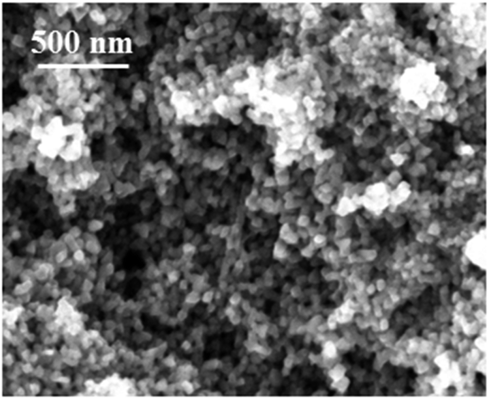
The cyclic voltammogram of Fe(TfO)₂/[Py_1,4]TfO on gold at a sweep rate of 10 mV s⁻¹ from OCP in the negative direction at 100 °C is shown in Fig. 1. Fig. 1 also shows the CV of [Py_1,4]TfO on gold at 100 °C as an inset. The CV shows several reduction processes (c₁ to c₅) in the cathodic branch and two oxidation processes in the anodic branch of the CV. The reduction wave c₁ is due to the reduction of Fe(III) to Fe(II). The reduction processes c₂–c₄ could be due to the underpotential deposition of Fe on gold or due to the alloying of gold with iron. The process c₅ (at ∼−1.5 V) is attributed to the reduction of Fe(II) to Fe. A crossover of forward scan with backward scan was also observed, which is attributed to a nucleation process. An oxidation process was observed at a₂ (∼−0.53 V) and is related to the partial oxidation of iron (Fe to Fe(II)). Furthermore, a broad oxidation wave was observed at a₁ (∼+0.28 V) which is obviously due to the oxidation of Fe(II) to Fe(III). The allocation of the reduction waves to definite processes is difficult. Several times we have experienced that the electrochemical behaviour of apparently simple compounds like e.g. Fe(TfO)₂ does not deliver a simple reduction process. This shows that – at a minimum – the surface processes upon deposition from ionic liquids are quite complicated and may be unique for each electrolyte. As our main interest for the present study was the deposition of materials, a controlled potentiostatic electrolysis was carried out to deposit Fe from 0.1 M Fe(TfO)₂ in [Py_1,4]TfO at an applied potential of −1.5 V for one hour on gold. The obtained deposit was washed with isopropanol followed by water and then analysed by scanning electron microscopy. An about 1–2 μm thick iron deposit was obtained on gold with very fine crystallite sizes in the nanometer regime (30 to 40 nm). Fig. 2 shows the SEM image of such a Fe deposit on gold at an applied potential of −1.55 V for one hour at 100 °C.

Fig. 1 Cyclic voltammogram of 0.1 M Fe(TfO)₂ in [Py_1,4]TfO on a polycrystalline gold electrode at 100 °C. ν = 10 mV s⁻¹. The CV of neat [Py_1,4]TfO on gold at 100 °C is shown in the inset.

Fig. 2 SEM image of the iron deposit on gold obtained from 0.1 M Fe(TfO)₂/[Py_1,4]TfO at 100 °C at −1.55 V.

Several iron deposits were prepared at various potentials from −1.25 V (sample 4) to −1.55 V (sample 1) on copper under similar conditions, whose magnetic hysteresis curves are shown in Fig. 3. The saturation polarisation of iron is J_s = 2.16 T,³ independent of the microstructure. The saturation polarisations of the hysteresis curves shown in Fig. 3 are considerably below this value indicating a high portion of a non-magnetic material. The ratio x of the measured polarisation J related to saturation polarisation J_s of pure iron x = J/J_s gives the portion of the magnetic iron material in the sample. This means that the magnetic portion of sample 1 with a saturation magnetization of J = 0.47 T consists of 21.8% iron. Furthermore, the thickness of the sample is below 2 μm, which leads to a high surface to volume ratio leading to a larger amount of less magnetic material in the deposit.

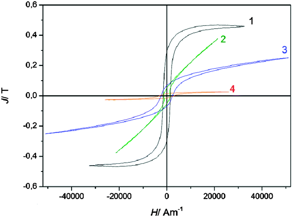Fig. 3 Magnetic hysteresis curves (magnetic polarisation J versus magnetic field strength H) of electrodeposited iron from 0.1 M Fe(TfO)₂/[Py_1,4]TfO at 100 °C with saturation polarisation far below saturation polarisation of pure iron indicating non-magnetic material in the samples (for further explanations see text).

While sample 1 and 4 show branches with nearly constant polarization at high magnetic fields, samples 2 and 3 are sheared (the branches are rotated from the x-axis). This is an indication for high inner demagnetizing fields^24,25 resulting from a porous granular material or by small magnetic particles embedded in a less magnetic phase. It is likely that a high fraction of hematite is present in the samples.

Thus, to improve the quality and thickness of the deposits, we employed FeCl₂ as a source of iron(II) species in the mentioned ionic liquid. Fig. 4 represents the cyclic voltammogram of 0.1 M FeCl₂/[Py_1,4]TfO on gold at a scan rate of 10 mV s⁻¹ at 100 °C. The electrode potential was scanned in negative direction from OCP as indicated by the arrows. The cyclic voltammogram on gold is characterized by 4 reduction and 2 oxidation processes. The process c₁ (at ∼+0.35 V) is due to reduction of Fe(III) to Fe(II) in the backward scan. As explained above, the processes in the CV are more complicated than expected. The onset of iron deposition was found to occur at ∼−1.1 V with a reduction peak at c₄ and we focussed here on the deposition of iron. Furthermore, a crossover is observed during scan reversal, which can be attributed to a nucleation process, with a nucleation overpotential of ∼0.32 V. Two oxidation waves a₂ (∼−0.18 V) and a₁ (∼+0.57 V) were observed in the anodic regime, which are due to oxidation of Fe to Fe(II) and Fe(II) to Fe(III), respectively. Wei et al. also observed a similar electrochemical behaviour for the deposition of Fe in [BMIm]BF₄.¹⁵

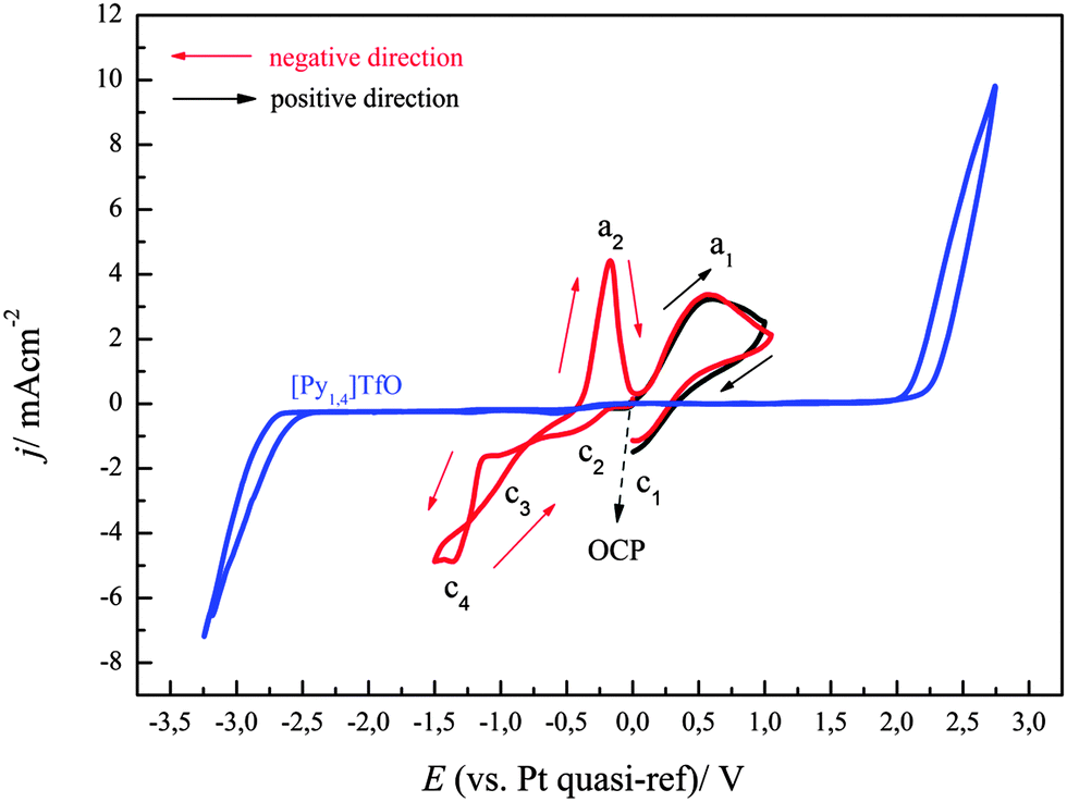Fig. 4 A comparison of two cyclic voltammograms of 0.1 M FeCl₂/[Py_1,4]TfO at 100 °C on polycrystalline gold in two different scan directions. Scan rate = 10 mV s⁻¹. The CV of neat [Py_1,4]TfO on gold at 100 °C is shown in blue colour.

Fig. 4 also shows the cyclic voltammogram of 0.1 M FeCl₂/[Py_1,4]TfO on gold at a scan rate of 10 mV s⁻¹ at 100 °C, where the electrode potential was initially scanned in a positive direction from OCP (black curve). Only one oxidation and one reduction process were observed, which are due to the oxidation of Fe(II) to Fe(III) and the reduction of Fe(III) to Fe(II), respectively. The CV of FeCl₂/[Py_1,4]TfO on copper will be discussed later.

To get more insight into the electrochemical behaviour of FeCl₂ in [Py_1,4]TfO, cyclic voltammograms were also recorded by scanning the electrode potential first in the positive direction from OCP. Fig. 5 shows the comparison of cyclic voltammograms of 0.1 M FeCl₂ in [Py_1,4]TfO that were recorded on gold at a scan rate of 10 mV s⁻¹ at 100 °C by scanning the electrode potential either in the positive or in the negative direction. The CV in negative direction (red) exhibits the same features as those observed in Fig. 4. If the potential is first scanned to the positive direction and reversed in the cathodic regime at −1.25 V (instead of −1.5 V), the peak at a₂ is seen as well but also a slight peak at a^I₂. Thus, Fe deposition occurs between −1.25 and −1.5 V and the peak a^I₂ seems to be due to underpotential deposition or alloying. Comparison of Fig. 1 with Fig. 4 and 5 shows that the oxidation process of Fe to Fe(II) is quite pronounced in the case of FeCl₂/[Py_1,4]TfO, compared to Fe(TfO)₂/[Py_1,4]TfO. This indicates that the dissolution of the deposited iron is more facile in FeCl₂/[Py_1,4]TfO than in Fe(TfO)₂/[Py_1,4]TfO. The different complexation of iron seems to be the determining factor.

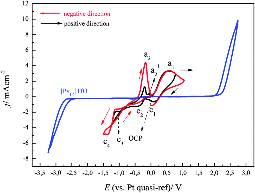Fig. 5 A comparison of cyclic voltammograms of 0.1 M FeCl₂/[Py_1,4]TfO in different scan directions at two different switching potentials on gold at a scan rate of 10 mV s⁻¹. Temperature = 100 °C. The line in blue colour represents the CV of neat [Py_1,4]TfO on gold at 100 °C.

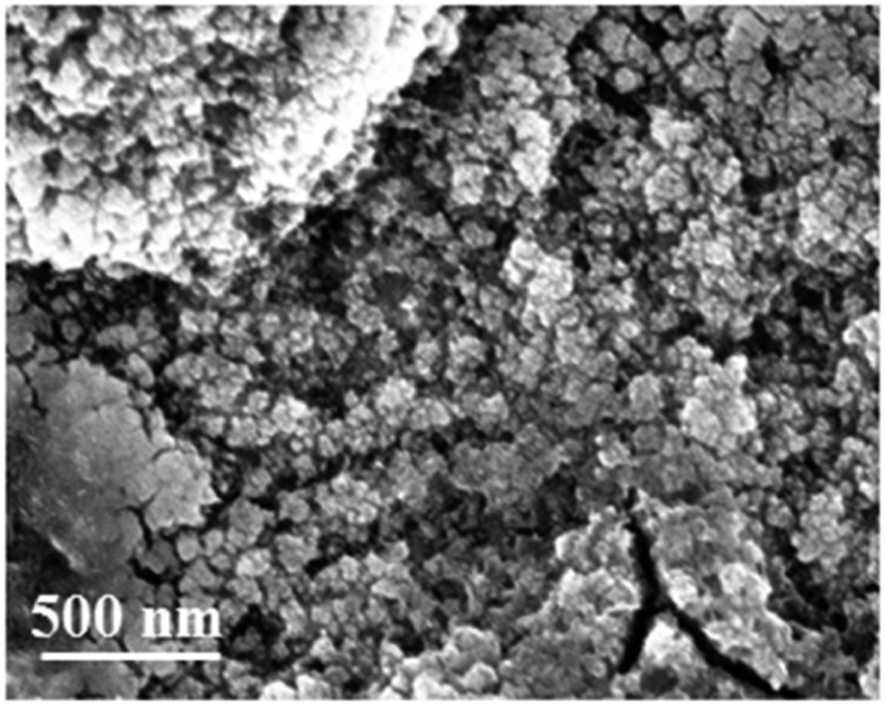
In order to make an iron deposit, potentiostatic electrolysis was carried out in 0.1 M FeCl₂/[Py_1,4]TfO at an electrode potential of −1.3 V for one hour on gold. The obtained deposit was washed subsequently with isopropanol and water and analysed by high resolution scanning electron microscopy and X-ray diffraction. Thick (∼10 μm) and smooth Fe deposits were obtained on gold. Fig. 6a and b show the SEM images of Fe deposits on gold and on copper, respectively. Uniform deposits were obtained on gold with very fine crystal sizes in the nanometer regime (40 to 50 nm). For XRD measurements, iron was electrodeposited on gold and on copper from 0.1 M FeCl₂ in [Py_1,4]TfO at an applied potential of −1.3 V for one hour at 100 °C. The obtained deposits were washed thoroughly in a stream of isopropanol followed by water.

Fig. 6 SEM images of iron deposits obtained from 0.1 M FeCl₂/[Py_1,4]TfO at −1.3 V at 100 °C (a) on gold and (b) on copper.

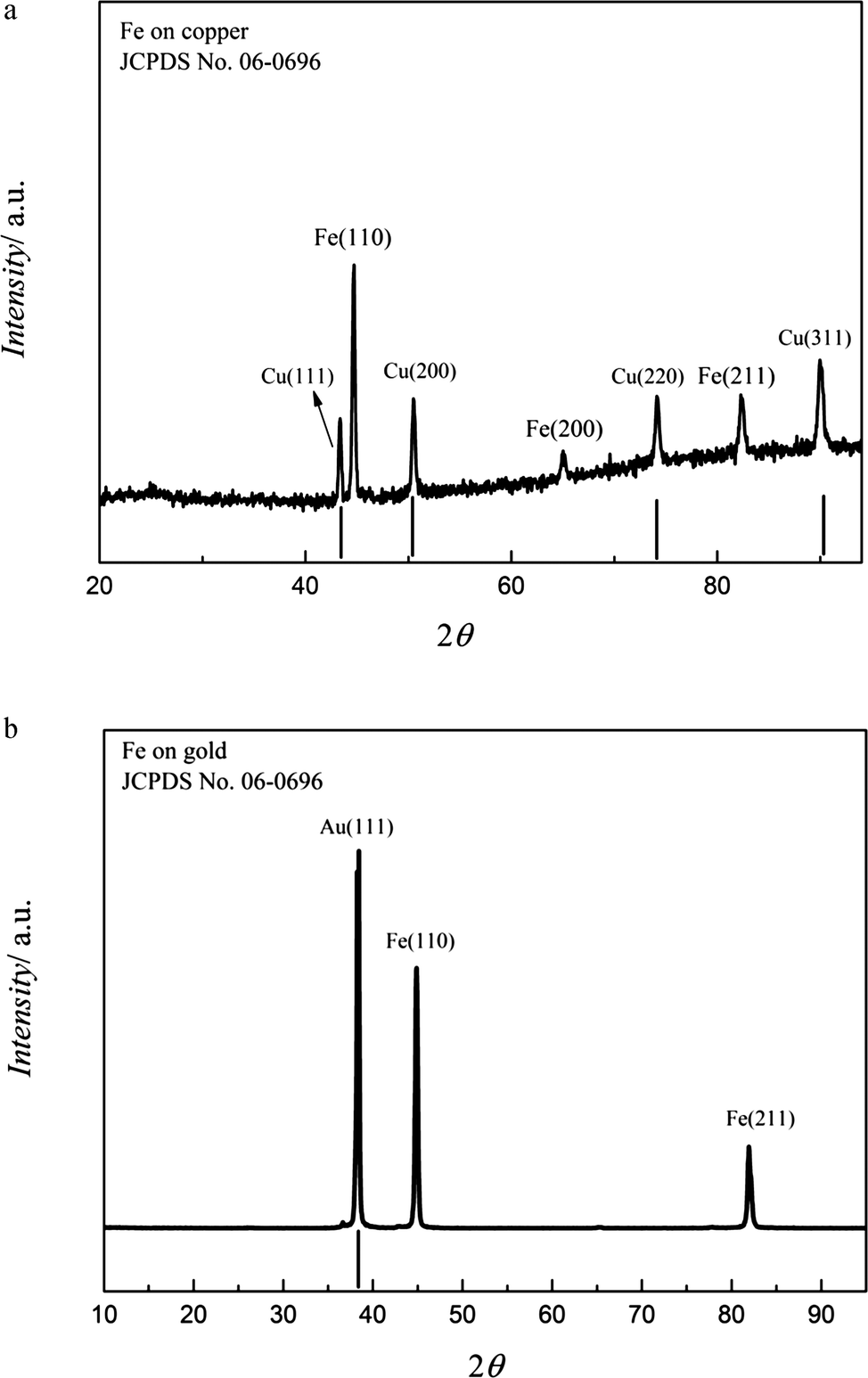
The washed samples were analysed by XRD and the data are shown in Fig. 7a. The bold vertical lines represent the patterns of the copper substrate. As seen, the obtained Fe deposit is crystalline and an intense (110) diffraction peak is obtained along with characteristic signals at (200) and (211). Furthermore, the diffraction peaks are relatively broad indicating a small crystal size. The average crystal size was found to be ∼50 to 60 nm using Scherrer equation.²⁶ The diffractogram of the iron deposit on gold from 0.1 M FeCl₂/[Py_1,4]TfO made at −1.3 V for one hour at 100 °C is shown in Fig. 7b. The deposit is crystalline and an intense (110) peak was observed in addition to the less intense (211) peak. The average crystal size was also found to be ∼50 to 60 nm.

Fig. 7 (a) XRD of the Fe deposit obtained on copper from 0.1 M FeCl₂/[Py_1,4]TfO at 100 °C at −1.3 V. (b) XRD of the iron deposit obtained on gold from 0.1 M FeCl₂/[Py_1,4]TfO at 100 °C at −1.3 V.

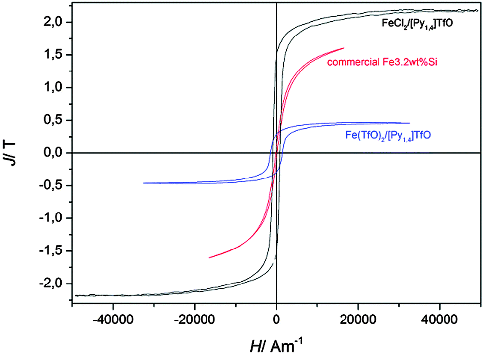
Fig. 8 shows magnetic measurements of such deposited iron samples. At first it is visible that the polarization of the pure iron sample shows a clearly higher polarisation than the hysteresis curve of the Fe3.2wt%Si reference sample. The saturation polarisation was estimated to be J_s,Fe = 2.1(±0.3) T which is close to the expected value of J_s = 2.16 T. Furthermore, the wider area of the hysteresis curve compared to the Fe3.2wt%Si sample is obvious, which is due to a much higher coercive force. This might be due to the small grain size of the electrodeposited iron sample, which is around 30–40 nm while the grains of the Fe3.2wt%Si sample are several millimeters wide. It is known in the literature that the coercive force is proportional to D⁶ between 10 and 100 nm and decreases with 1/D with increasing grain sizes D > 100 nm, while it is zero for single domain grains.⁵ The theoretical grain size of an iron single domain particle is 3 nm, while experimentally a size of 6 nm could be estimated.²⁷ In our iron sample we found a coercive force of H_c = 920 A m⁻¹, which corresponds to a grain size of approximately d = 50 nm.^5,28 The coercive force is given by the intersection of the hysteresis curve with the abscissa and was estimated numerically from measurement values.

Fig. 8 Comparison of hysteresis curves (magnetic polarisation J versus magnetic field strength H) of commercially available highly grain oriented electrical steel (Fe3.2wt%Si, thickness d = 230 μm, coated with Forsterite) and electrodeposited iron. For comparison purposes curve 1 of Fig. 3 is also shown here.

The frequency dependency of the hysteresis curves for magnetizing frequencies in the range of 100 Hz and 1000 Hz for the pure iron, deposited from FeCl₂/[Py_1,4]TfO, is shown in Fig. 9. The frequency dependent coercive force H_c(f) = H_exc(f) + H₀ remains nearly constant at approximately H_c = 950 A m⁻¹ for all measurements. H₀ is the mean value of the coercive force depicting the mean domain wall hindrance by lattice imperfections in the case of a constant external magnetic field and a constant domain wall velocity, or expressed more simply, the coercive force measured in a nearly static field with a magnetizing frequency f = 0 Hz. The excess field H_exc is the remaining field acting in the magnetization process on single domain walls, groups of domain walls and/or domain wall segments needing higher activation energies.^29,30 The movement of these magnetic objects generates micro eddy currents at higher magnetizing frequencies leading to a higher frequency dependent coercive force H_c(f) and additional power losses. A movement of the domain walls with a nearly constant velocity in our measurements can be assumed because the coercive force does not considerably change with frequency.

Fig. 9 Frequency dependent magnetic hysteresis curves (magnetic field strength H versus magnetic polarisation J) of electrodeposited iron samples. Hysteresis curves for magnetizing frequencies f = 50 Hz, and f = 200 Hz are not shown here for reasons of clarity as they cannot be clearly distinguished from the curves shown here.

The power losses per magnetization cycle are related to the area of the hysteresis curves and were estimated numerically by the measurement software to be P (f = 50 Hz) = 6500 J m⁻³ and increasing with magnetizing frequency to P (f = 100 Hz) = 9500 J m⁻³. Since the hysteresis curves at frequencies 300 Hz ≤ f ≤ 1000 Hz were measured at lower polarisation, power losses are lower and therefore not shown here.

Electrodeposition of aluminium

The electrodeposition of Al in AlCl₃/[Py_1,4]TfO has been described in our previous article.¹⁸ Here, we only describe the deposition of Al on mild steel in 2.75 M AlCl₃ in [Py_1,4]TfO. The cyclic voltammogram of 2.75 M AlCl₃ in [Py_1,4]TfO on mild steel at 100 °C is shown in Fig. 10. A reduction wave was observed due to the bulk deposition of aluminium and the corresponding stripping peak was observed at 0.25 V.

Fig. 10 Cyclic voltammogram of 2.75 M AlCl₃/[Py_1,4]TfO on mild steel at 100 °C at a scan rate of 10 mV s⁻¹. The CV of neat [Py_1,4]TfO on gold at 100 °C is shown in red colour.

A potentiostatic electrolysis was carried out to deposit aluminium from 2.75 M AlCl₃ in [Py_1,4]TfO at an electrode potential of −1.25 V for one hour at 100 °C on mild steel. The obtained deposit was washed with isopropanol followed by water and then analysed by high resolution scanning electron microscopy. A thick and smooth aluminium deposit was obtained on mild steel. Fig. 11 represents the SEM image of such an aluminium deposit. A uniform and thick aluminium deposit was obtained with very fine crystallite sizes in the nanometer regime (40 to 50 nm).

Fig. 11 Microstructure of Al electrodeposit on mild steel obtained from AlCl₃/[Py_1,4]TfO at 100 °C for one hour.

The XRD patterns of the electrodeposited aluminium at an applied potential of −1.25 V on mild steel for one hour is shown in Fig. 12. As seen from the figure, the deposited aluminium is crystalline and a strong (111) diffraction peak is obtained along with the other characteristic diffraction peaks (200), (220), (311), and (222). Furthermore, the diffraction peaks are broad and thus indicate a small crystal size of the aluminium deposit. The average crystal size was found to be ∼40 to 50 nm from Scherrer equation, which is in good agreement with the SEM images.

Fig. 12 XRD of the Al deposit obtained on gold from 2.75 M AlCl₃/[Py_1,4]TfO at 100 °C at −1.25 V.

Electrodeposition of iron–aluminium alloys

A solution of (0.1 M FeCl₂ + 2.75 M AlCl₃)/[Py_1,4]TfO was prepared and used for the electrodeposition of Fe–Al alloys. As this mixture is solid at room temperature, the electrochemical experiments were performed at 100 °C. The cyclic voltammogram at 100 °C on gold at a scan rate of 10 mV s⁻¹ from OCP in the negative direction is shown in Fig. 13. The dashed curve shows a cyclic voltammogram, which was initially scanned in the positive direction from OCP. An oxidation wave at a₁ (∼+0.2 V) and an associated reduction wave at c₁ were observed due to the redox couple Fe(II)/Fe(III).

Fig. 13 A comparison of two cyclic voltammograms of 0.1 M FeCl₂/[Py_1,4]TfO at 100 °C on polycrystalline Au in two different scan directions. Scan rate = 10 mV s⁻¹. The CV of neat [Py_1,4]TfO on gold at 100 °C is shown in black colour.

The solid curve (red colour) represents the CV that was initially swept in the negative direction. A reduction wave is observed at c₂, which is due to the bulk deposition of iron. The oxidation process a₂ (at ∼−0.38 V) is correlated with the dissolution of deposited iron. The onset of iron deposition was found to occur at ∼−0.52 V. A distinct current loop is observed in the reverse scan, which can be attributed to nucleation processes. We neither observed underpotential deposition of iron on gold nor alloying of iron with gold from (0.1 M FeCl₂ + 2.75 M AlCl₃)/[Py_1,4]TfO. In contrast, we observed such surface processes on gold from 0.1 M FeCl₂ alone in [Py_1,4]TfO. The presence of AlCl₃ introduces Cl⁻ which obviously makes the electrochemistry reversible.

The cyclic voltammograms of (0.1 M FeCl₂ + 2.75 M AlCl₃)/[Py_1,4]TfO on gold at 100 °C were recorded at different switching potentials at a sweep rate of 10 mV s⁻¹ and are depicted in Fig. 14. The cyclic voltammograms on gold exhibit a reduction wave between ∼−0.5 and −1.5 V with the corresponding oxidation processes between ∼−0.45 and ∼0.15 V, varying with the switching potential. If the switching potential is set below ∼−1.05 V, a slight increase in the reduction current and a distinct reduction process (at c₃) are observed due to Fe–Al codeposition. However, no distinct oxidation waves are observed for the dissolution of Fe–Al deposits, which might presumably be merged with the dissolution peaks of iron. Instead, we observed broad oxidation waves in the potential region between ∼−0.45 V and +0.15 V. If the switching potential is set below ∼−1.85 V another reduction wave (at c₄) is observed due to the bulk deposition of aluminium. The onset of iron–aluminium codeposition was found to be around −0.95 V and the onset of bulk aluminium deposition was found to be ∼−1.9 V.

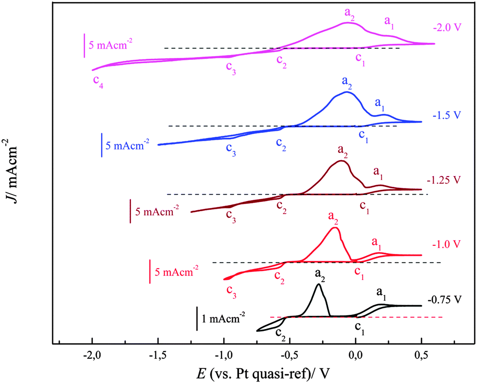Fig. 14 A comparison of five cyclic voltammograms of 0.1 M FeCl₂/[Py_1,4]TfO at 100 °C on polycrystalline Au at various switching potentials. Scan rate = 10 mV s⁻¹.

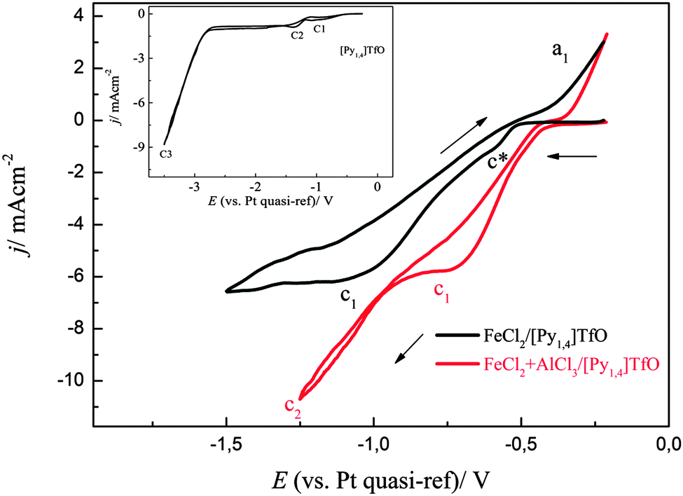
A comparison of two cyclic voltammograms of (0.1 M FeCl₂)/[Py_1,4]TfO and (0.1 M FeCl₂ + 2.75 M AlCl₃)/[Py_1,4]TfO on copper is shown in Fig. 15. The CV of (0.1 M FeCl₂)/[Py_1,4]TfO exhibits two reduction processes and one oxidation process. The shoulder at c* might be due to surface alloying of iron with copper and the reduction peak at c₁ is due to the bulk deposition of iron. The process at a₁ is due to the dissolution of iron. Two distinct reduction processes were seen in the CV of (0.1 M FeCl₂ + 2.75 M AlCl₃)/[Py_1,4]TfO, which are attributed to the deposition of iron and the codeposition of iron and aluminium, respectively. The oxidation process at a₁ is correlated with the dissolution of iron and of iron–aluminium. The inset of Fig. 15 shows the CV of neat [Py_1,4]TfO on copper at 100 °C.

Fig. 15 A comparison of two cyclic voltammograms of 0.1 M FeCl₂/[Py_1,4]TfO and (0.1 M FeCl₂ + 2.75 M AlCl₃)/[Py_1,4]TfO at 100 °C on copper at two different switching potentials. Scan rate = 10 mV s⁻¹. The CV of neat [Py_1,4]TfO on copper at 100 °C is shown in the inset.

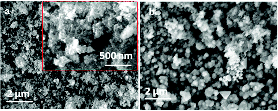
In the following, constant-potential electrolysis was carried out to deposit iron and iron–aluminium alloys from the employed electrolyte at various applied potentials ranging from −0.65 V to −1.4 V on gold for one hour. The obtained deposits were washed with isopropanol followed by distilled water and analysed by high resolution scanning electron microscopy, X-ray diffraction and EDX. Visually, thick (∼10 μm) and uniform iron deposits were obtained, and the corresponding SEM micrographs are shown Fig. 16. The SEM micrograph of the gold substrate is shown in Fig. 16a along with its high-resolution in the inset. The SEM micrograph of the deposit at a potential of −0.65 V shows agglomerated spherical structures along with fine particles (Fig. 16b).

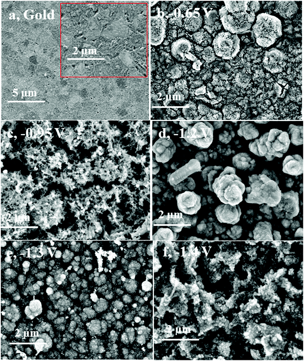Fig. 16 SEM micrographs of iron–aluminium deposited on gold in (0.1 M FeCl₂ + 2.75 M AlCl₃)/[Py_1,4]TfO at 100 °C. At (a) gold substrate and the inset shows its high-resolution image (b) −0.65 V, (c) −0.95 V (Al wt% = 1), (d) −1.2 V (Al wt% = 4.7), (e) −1.3 V (Al wt% = 7.4), and (f) −1.4 V (Al wt% = 10.1).

At the applied potential of −0.95 V, both the particle size and the extent of agglomeration are decreased, and the corresponding SEM micrograph is shown in Fig. 16c. The Al content was found to be 1 wt%. While at the deposition potential of −1.2 V (∼4.7 wt%), the deposit is denser with an increased agglomeration (Fig. 16d), at the potentials −1.3 V and −1.4 V the particle size and agglomeration again are significantly decreased (see Fig. 16e and f). This can be due to an increase in the aluminium content in the deposits. Small crystals are seen in the SEM micrographs at potentials of −1.3 V (Fig. 16e) and −1.4 V (Fig. 16f). The aluminium content in the deposits gradually increases from 3.1 to 10.1 wt% upon changing the deposition potential from −1.1 to −1.4 V, respectively.

The SEM image of the copper substrate is shown in Fig. 17a. Fig. 17b–f show the SEM micrographs of iron–aluminium deposits obtained on copper at various potentials ranging from −0.7 V to −1.4 V for one hour at 100 °C. Thick and uniform deposits were obtained on copper, too. The respective SEM images are presented in Fig. 17b–f. The aluminium content was found to increase from 4.6 wt% to 10.5 wt% upon varying the deposition potentials from −1.2 V to −1.4 V, respectively, whereas at −0.7 V only iron and at −1 V iron and a small amount of Fe₃Al could be obtained in the deposits, respectively.

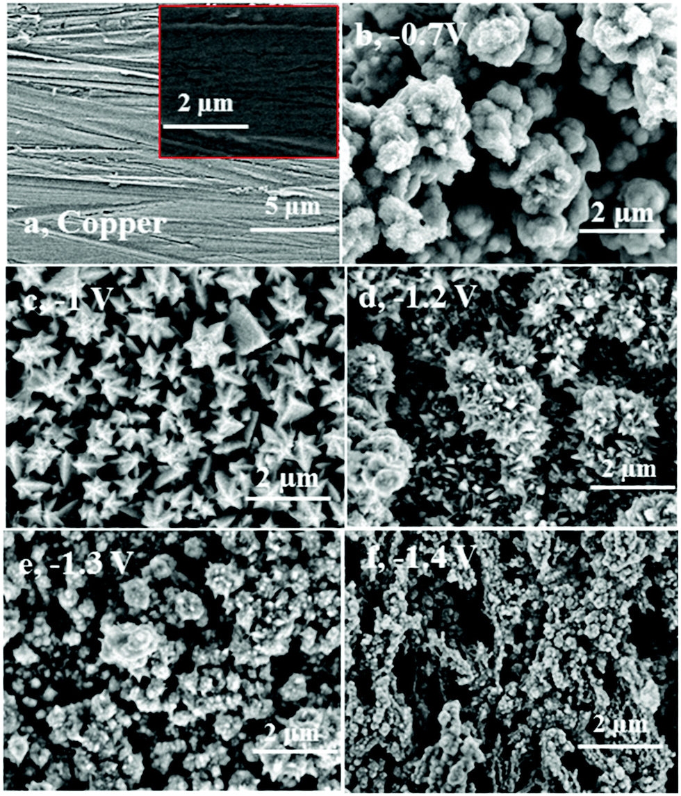Fig. 17 SEM micrographs of iron–aluminium deposits obtained on copper from (0.1 M FeCl₂ + 2.75 M AlCl₃)/[Py_1,4]TfO at 100 °C. At (a) copper substrate and the inset shows its high-resolution image (b) −0.7 V, (c) −1.0 V (Al wt% = 1.1), (d) −1.2 V (Al wt% = 4.6), (e) −1.3 V (Al wt% = 7.8), and (f) −1.4 V (Al wt% = 10.5).

For an XRD analysis, iron–aluminium alloys were electrodeposited on gold from (0.1 M FeCl₂ + 2.75 M AlCl₃)/[Py_1,4]TfO at various applied potentials at 100 °C. The deposits were thoroughly washed and analysed by XRD, the patterns of iron–aluminium deposits on gold are shown in Fig. 18. At an applied potential of −0.95 V, two intense diffraction peaks are seen and attributed to the Fe(110) and Fe(211) planes along with a low intensity peak due to an iron–aluminium alloy (with an average composition of ∼Al_3.2Fe). In the case of the deposit obtained at −1.1 V, the mentioned two strong diffraction peaks for Fe(110) and Fe(211) together with two peaks due to iron–aluminium alloys, i.e. Fe₃Al (JCPDS No. 06-0695) and Al_3.2Fe (JCPDS No. 38-1147), are observed. Furthermore, the intensities of iron–aluminium peaks increase when making the deposition potential more negative.

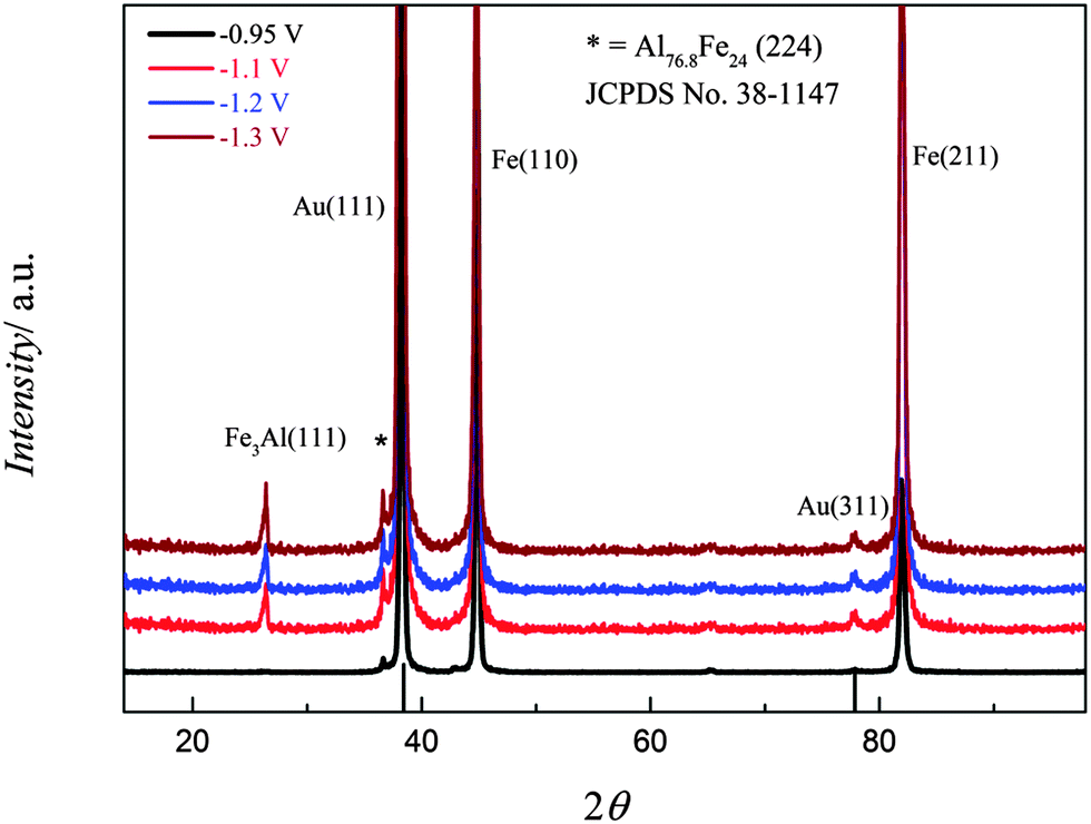Fig. 18 XRD of the iron–aluminium deposited on gold from (0.1 M FeCl₂ + 2.75 M AlCl₃)/[Py_1,4]TfO at four different applied potentials: T = 100 °C.

XRD patterns of iron–aluminium deposits at four different deposition potentials on copper at 100 °C are shown in Fig. 19. The peak intensities of the iron–aluminium alloy (Fe₃Al, JCPDS No. 06-0695) gradually increases upon varying the deposition potentials from −1.0 to −1.4 V. The Fe(110) is observed whereas Fe(211) and the peak due to Al_3.2Fe are missing.

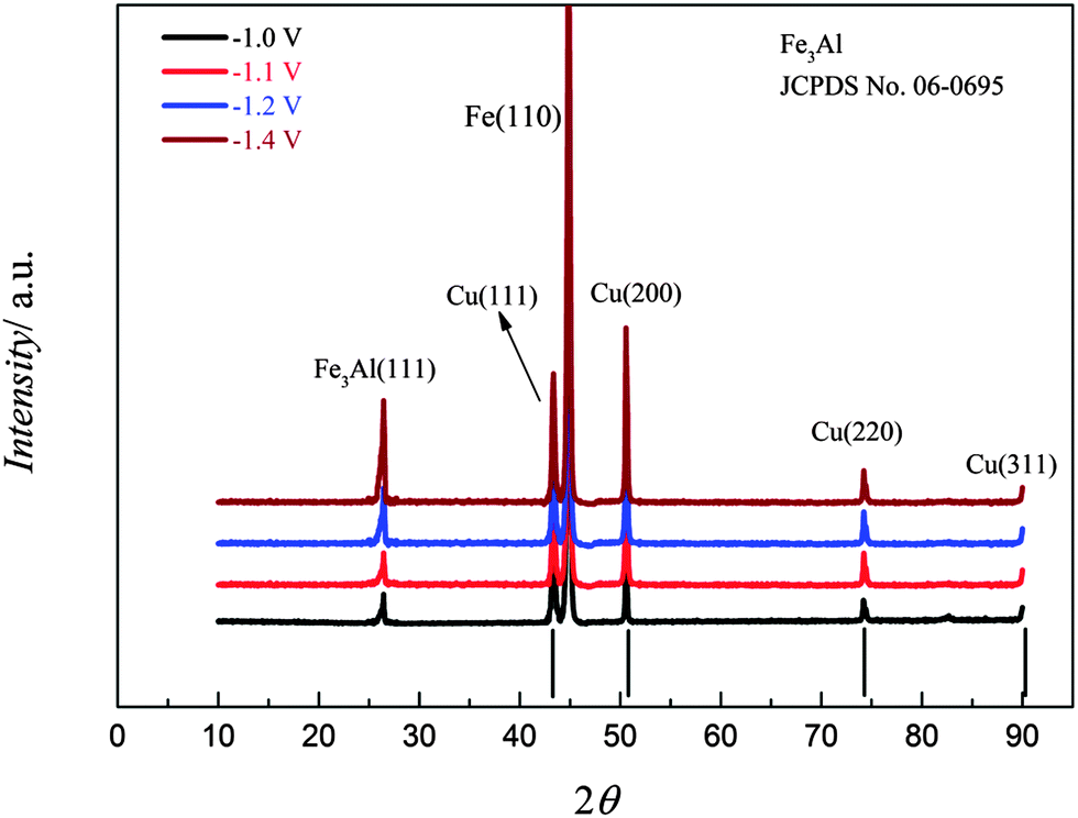Fig. 19 XRD of the iron–aluminium deposits on copper obtained from (0.1 M FeCl₂ + 2.75 M AlCl₃)/[Py_1,4]TfO at various deposition potentials at 100 °C.

Fig. 20 shows the magnetic hysteresis curves of electrodeposited pure iron at −0.65 V and of the iron–aluminium alloy at −1.2 V (4.6 wt%). It can be seen that the saturation polarisation is decreased by alloying iron with aluminium. The saturation polarisation of the iron–aluminium alloy was estimated to be J_s(Al) = 1.8 T. This corresponds to an aluminium content of around 4.5 wt%,³¹ which is in good agreement with the composition. The coercive force is H_c = 1050 A m⁻¹, which is slightly higher than the coercive force of the pure iron sample (H_c,Fe = 950 A m⁻¹) indicating a mean grain size of approximately d = 75 nm. The frequency dependent hysteresis curves of iron–aluminium deposited at −1.2 V are presented in Fig. 21. Like for pure iron samples, the coercive force for the Fe–Al alloy remains nearly constant at approximately H_c = 1050 A m⁻¹ for all magnetizing frequencies. The power loss at a magnetizing frequency f = 100 Hz are P = 12 800 J m⁻³, which is a little bit higher than the power loss in pure iron at the same magnetizing frequency. This might be due to the higher coercive force for the larger grains.

Fig. 20 Comparison of magnetic hysteresis curves (magnetic field strength H versus magnetic polarisation J) of electrodeposited iron and iron–aluminium alloy.

Fig. 21 Frequency dependent magnetic hysteresis curves (magnetic field strength H versus magnetic polarisation J) of electrodeposited iron–aluminium alloy. For reasons of clarity, hysteresis curves for magnetizing frequencies f = 50 Hz, f = 300 Hz, and f = 1000 Hz are not shown.

Conclusions

The electrodeposition of iron and iron–aluminium was investigated in [Py_1,4]TfO on gold and on copper at 100 °C. From the above results, the following features can be summarized. The voltammogram of Fe(TfO)₂/[Py_1,4]TfO exhibits several difficult to allocate reduction processes in the cathodic branch whereas the voltammogram of FeCl₂/[Py_1,4]TfO exhibits mainly one strong reduction peak along with a few surface reduction processes. The dissolution of the deposited iron is clearly seen in the CV of FeCl₂/[Py_1,4]TfO while the dissolution of iron is hindered in Fe(TfO)₂/[Py_1,4]TfO. Thin iron deposits were obtained on copper from Fe(TfO)₂/[Py_1,4]TfO, showing a poor magnetic response, which might either be due to the low thickness or due to the presence of non-magnetic species in the deposit. However, ∼10 μm thick iron and iron–aluminium deposits were obtained on copper from FeCl₂/[Py_1,4]TfO and from (FeCl₂ + AlCl₃)/[Py_1,4]TfO, respectively. XRD results reveal that two types of iron–aluminium alloys (Fe₃Al and Al_3.2Fe) were obtained on gold at the studied temperature together with iron. However, only one alloy (Fe₃Al) was obtained on copper at the same temperature.

As expected from the grain size dependence of the coercive force for nanocrystalline materials, the coercive force of our samples is relatively high around H_c = 1000 A m⁻¹, indicating grain sizes of 50–75 nm. It is shown that the preparation of typical magnetic alloys with a low thickness is feasible and it can be expected that an optimization of grain sizes and compositions of the magnetic alloys will lead to soft magnetic materials with good magnetic properties.

References

1. F. J. Himpsel, J. E. Ortega, G. J. Mankey and R. F. Willis, Adv. Phys., 1998, 47, 511.
2. H. B. Peng, T. G. Ristroph, G. M. Schurmann, G. M. King, J. Yoon, V. Narayanamurti and J. A. Golovchenko, Appl. Phys. Lett., 2003, 83, 4238.
3. R. M. Bozorth, Ferromagnetism, IEEE Press, New York, 1978.
4. A. Hernando, J. Phys.: Condens. Matter, 1999, 11, 9455.
5. G. Herzer, IEEE Trans. Magn., 1990, 26, 1397.
6. M. J. Aus, C. Cheung, B. Szpunar, U. Erb and J. Szpunar, J. Mater. Sci. Lett., 1998, 17, 1949.
7. J. L. McCrea, G. Palumbo, G. D. Hibbard and U. Erb, Rev. Adv. Mater. Sci., 2003, 5, 252.
8. Y. Castrillejo, A. M. Martinez, M. Vega and P. S. Batanero, J. Appl. Electrochem., 1996, 26, 1279.
9. A. Lugovskoy, M. Zinigrad, D. Aurbach and Z. Unger, Electrochim. Acta, 2009, 54, 1904.
10. C. Nanjundiah, K. Shimizu and R. A. Osteryoung, J. Electrochem. Soc., 1982, 129, 2474.
11. T. M. Laher and C. L. Hussey, Inorg. Chem., 1982, 21, 4079.
12. M. Lipsztajn and R. A. Osteryoung, Inorg. Chem., 1985, 24, 716.
13. S. Pye, J. Winnick and P. A. Kohl, J. Electrochem. Soc., 1997, 144, 1933.
14. J. F. Huang and I. W. Sun, J. Electrochem. Soc., 2004, 151, C8.
15. Y. M. Wei, X. S. Zhou, J. G. Wang, J. Tang, B. W. Mao and D. M. Kolb, Small, 2008, 4, 1355.
16. H. Y. Huang, C. J. Su, C. L. Kao and P. Y. Chen, J. Electroanal. Chem., 2010, 650, 1.
17. H. R. Zhou, Y. D. Yu, G. Y. Wei and H. L. Ge, Int. J. Electrochem. Sci., 2012, 7, 5544.
18. P. Giridhar, S. Zein El Abedin and F. Endres, J. Solid State Electrochem., 2012, 16, 3487.
19. Q. Zhu, C. L. Hussey and G. R. Stafford, J. Electrochem. Soc., 2001, 148, C88.
20. W. R. Pitner, C. L. Hussey and G. R. Stafford, J. Electrochem. Soc., 1996, 143, 130.
21. M. R. Ali, A. Nishikata and T. Tsuru, Electrochim. Acta, 1997, 42, 1819.
22. R. T. Carlin, P. C. Trulove and H. C. De Long, J. Electrochem. Soc., 1996, 143, 2747.
23. R. T. Carlin, H. C. De Long, J. Fuller and P. C. Trulove, J. Electrochem. Soc., 1998, 145, 1598.
24. M. Anhalt and B. Weidenfeller, J. Appl. Phys., 2009, 105, 113903.
25. M. Anhalt, B. Weidenfeller and J. L. Mattei, J. Magn. Magn. Mater., 2008, 320, e844.
26. P. Scherrer, Göttinger Nachrichten, 1918, 2, 98.
27. A. F. Rodriguez, A. Kleibert, J. Bansmann, A. Voitkans, L. J. Heyderman and F. Nolting, Phys. Rev. Lett., 2010, 104, 127201.
28. B. Weidenfeller, Magnetic Properties of Polymer Bonded Soft Magnetic Composites, Papierflieger, Clausthal-Zellerfeld, 2008.
29. H. J. Williams, W. Shockley and C. Kittel, Phys. Rev., 1950, 80, 1090.
30. B. Weidenfeller and W. Rieheman, J. Magn. Magn. Mater., 1996, 160, 136.
31. F. Pawlek, Magnetische Werkstoffe, Springer, Berlin-Göttingen-Heidelberg, 1952.

---