Non-uniform spatial distribution of tin oxide (SnO₂) nanoparticles at the air–water interface

Abstract

Depth resolved X-ray photoelectron spectroscopy (XPS) combined with a 25 μm liquid jet is used to quantify the spatial distribution of 3 nm SnO₂ nanoparticles (NPs) from the air–water interface (AWI) into the suspension bulk. Results are consistent with those of a layer several nm thick at the AWI that is completely devoid of NPs.

---

The attachment of NPs at liquid interfaces is a central topic in colloid science but remains poorly understood.¹ From a fundamental standpoint, a well-defined NP at the air–liquid interface is viewed as an ideal system to investigate thermodynamic models, surface free energies, electrostatic interactions, capillary and solvation forces, line tensions, and phase behaviour.¹ Interest also arises from the commercial industry where NPs at liquid interfaces have applications in stabilizing emulsions, foams, and microbubbles^2–4 that are commonplace in food, paint and cosmetics.⁵ More recently, the nanotechnology sector has shown interest in NPs at liquid interfaces as a means to assemble complex 2d and 3d nanocrystal superlattices that possess unique chemical and physical properties for applications in electronic and optoelectronic devices such as LEDs, lasers, and solar cells.⁶

The attachment of NPs at air–liquid interfaces, that is their surface affinity, is traditionally characterized using surface tension measurements. These measurements rely on the Gibbs absorption equation⁷ to calculate the interface density (Γ) from the recorded change in surface tension (dγ) with a change in chemical potential (dμ) of the adsorbing NPs, and have been performed successfully for over a half century.⁸ While limitations such as a lack of chemical and depth (subsurface) resolution precludes surface tension measurements from providing a complete microscopic description of the NP attachment at and near the air–liquid interface, few analytic techniques offer improvement. With a clear desire to better understand the NP attachment at liquid interfaces, more refined microscopic probes are sought. To date, cryogenic electron tomography has been the most successful technique and has recently been used to quantify the complete concentration gradient of oleic acid stabilized 5 nm PbSe NPs at the air–organic solvent interface.⁹ Spectroscopic approaches have remained to date largely unexplored.¹⁰

X-ray photoelectron spectroscopy (XPS) is a quantitative tool that offers depth resolution. By carrying out experiments as a function of incident photon energy, afforded by, for example, a synchrotron radiation facility, the probe depth of the experiment can be carefully controlled via the inelastic mean free path (IMFP)¹¹ of the outgoing photoelectron. Probe depths from a few molecular layers up to several tens of nm can be realized.¹¹ Only recently, however, has XPS been extended to aqueous samples using a liquid microjet¹² and its application to study the three-way interface of air–water–NPs is a relatively virgin discipline^13–16 with but a single depth-resolved study that did not attempt to quantify NP spatial distributions.¹⁷ Here we combine XPS with a liquid microjet operating on a colloidal SnO₂ suspension to measure depth-resolved NP spatial distributions at the AWI. The present report is the first attempt to quantify NP spatial distributions at the AWI using a spectroscopic method.

Our experimental model system consists of charge-stabilized colloidal SnO₂. These NPs are ligand-free and rely on the electric field generated at the surface of the particle by (de)protonated hydroxyl groups for stability. SnO₂, a wide band gap semiconductor, has applications in gas sensing, catalysis, electrochemistry, and optoelectronic devices.¹⁸ Colloidal suspensions of SnO₂ are used to generate nanocrystalline thin films that have been successful in dye sensitization for solar cell technology.¹⁹ As such, a microscopic description of SnO₂ NPs in liquid solutions will benefit several scientific disciplines of current significance.

The setup of our liquid microjet experiment at the SIM beamline²⁰ of the Swiss Light Source is shown in Fig. 1. The experiment uses a NAPP spectrometer²¹ operating at a constant pass energy of 50 eV for all photoelectron kinetic energies (pKE). The direction of the liquid microjet flow, incident photon, and photoelectron detection are orthogonal (inset of Fig. 1). Suspensions of 7 wt% SnO₂ are prepared by diluting a commercially available 15 wt% sample (Nyacol SN15). The suspension pH is 10.5 and particle diameters are 3.0 ± 1.6 nm as determined by in situ small angle X-ray scattering (ESI†). Representative TEM micrographs of dried (ex situ) aliquots of the suspension are provided in the ESI.† Sn 3d_5/2 spectra are collected using a 25 μm liquid jet operating at 279 K and a flow rate of 0.4 mL min⁻¹. The diameter of the liquid jet, the liquid flow rate, and the pressure inside the ionization chamber are not expected to influence the results of the present study.¹³ Measurements are carried out at pKEs of 110, 210, 310, 435, 580, and 810 eV using incident photon energies of 600, 700, 800, 925, 1070, and 1300 eV, respectively. Collection time is typically 25 min per spectrum, although at pKEs of 110 and 210 eV, the signal is averaged for 50 min to increase the signal to noise ratio. The probe depth of the experiment is a strong function of the pKE²¹ and is only beginning to be understood in aqueous solutions.²² A well-pronounced minimum is believed to occur at around 100 eV,²¹ and upon increasing pKE the probe depth increases. We used IMFPs of 7.8 Å (110 eV pKE), 10.4 Å (210 eV), 13.3 Å (310 eV), 17.0 Å (435 eV), 19.5 Å (580 eV), and 27.2 Å (810 eV).²²

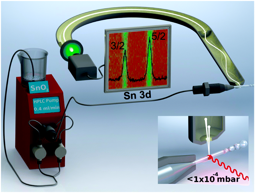Fig. 1 Setup used to perform depth-resolved X-ray photoelectron spectroscopy measurements at the three-way interface of air–water–nanoparticles. Colloidal suspensions of 7.5 wt% SnO₂ are injected into the measurement chamber using a fused quartz capillary with a diameter of 25 μm. (inset) Experimental geometry.

Fig. 2 shows the as-collected Sn 3d_5/2 spectra at pKE of (a) 110, (b) 210, (c) 310, (d) 435, (e) 580, and (f) 810 eV. Relatively poor signal quality (despite the highest photon flux and photoionization cross-section²³) at 110 eV pKE is a direct reflection of the spatial distribution of the NPs at the AWI (vide infra). The complete Sn 3d orbital with both the 3d_5/2 and 3d_3/2 components is shown in Fig. 1. Here we use only the 3d_5/2 component for determining SnO₂ NP spatial distributions at the AWI. The XP spectra can be quantified by normalizing the integrated intensity following background subtraction to the photon flux, the photoionization cross-section,²³ and to the transmission function of the hemispherical NAPP spectrometer. The normalized intensity is shown in Fig. 3a (black markers) as a function of IMFP. The value at 27.2 Å (810 eV pKE) has been set to unity for simplicity. The normalized intensity is relatively flat between 7 and 13 Å after which it increases sharply up to 27.2 Å. Error bars represent the standard deviation of repeat measurements.

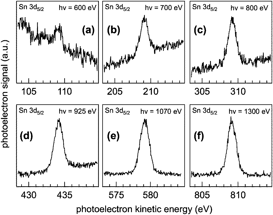Fig. 2 Sn 3d_5/2 XP spectra as a function of photoelectron kinetic energy (pKE). (a) 110 eV, (b) 210 eV, (c) 310 eV, (d), 435 eV, (e) 580 eV, and (f) 810 eV. Raw data are shown. To quantify the spectral intensity, a Gaussian function is fit to each spectrum following a linear background subtraction and the integrated intensity is normalized to the photon flux, the photoionization cross section, and analyser transmission function.

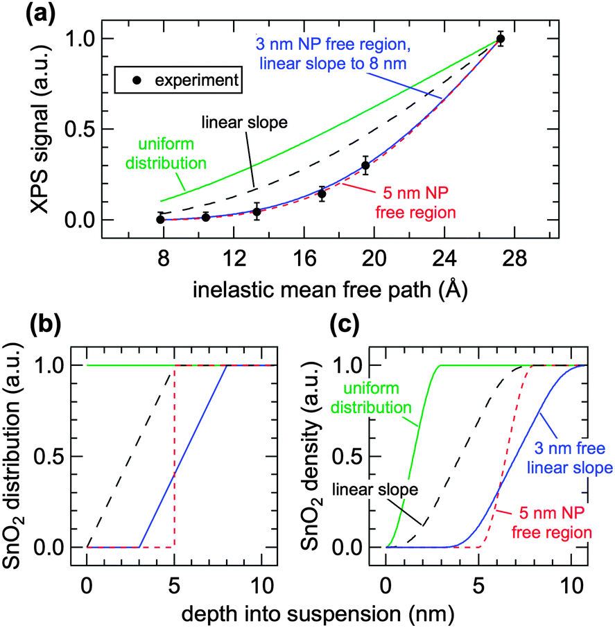Fig. 3 (a) Measured (markers) and calculated (lines) signal intensities as a function of inelastic mean free path (IMFP). (b) Four different NP spatial distribution models and (c) their corresponding density profiles. The air–water interface is at a depth of 0 nm in (b) and (c).

The normalized XPS intensities as a function of IMFP can be compared with the predicted signals from different NP distributions at the AWI. A uniform distribution of randomly oriented SnO₂ NPs (Fig. 3b, green trace) from the AWI into the bulk gives rise to the density profile shown in Fig. 3c (green trace, uniform distribution). The bulk suspension SnO₂ density is realized at a depth below the AWI equal to the NP diameter (in this case 3 nm). The density profile of the uniform NP distribution can be integrated using well-established methods^{14,17,24–26} to generate a predicted XPS intensity as a function of IMFP that can be directly compared with the experimental values. The integral takes the form 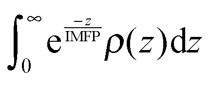where IMFP is the inelastic mean free path, z is the distance into the suspension from the AWI, and ρ(z) is the SnO₂ density at a given depth. The limits of the integral are from the AWI to the bulk. In theory, this calculation is a double integral¹⁷ where an IMFP for SnO₂ is first used to calculate the attenuation of the PE within the NP, and a second integral uses IMFP for liquid water to account for further attenuation in the condensed liquid phase before the PE escapes into vacuum. In practice, and as we have shown in the ESI,† variations of ±25% in the IMFP have very little effect on the results of this study and the equation can be simplified to the single integral shown. The predicted XPS intensity for a uniform NP distribution over IMFP spanning the experimental range is shown in Fig. 3a (green trace, uniform distribution). The experimental intensities are grossly overestimated for all IMFPs. This result suggests that the NPs do not have a uniform distribution near the AWI but are instead depleted relative to the bulk. Density profiles (Fig. 3c) and predicted XPS intensities (Fig. 3a) have been similarly calculated for NP distributions (Fig. 3b) that include a 5 nm thick region at the AWI where the NPs are completely excluded followed by a step function increase in distribution to the bulk value (red dotted trace), for a linear increase in NP distribution from a zero depth to 5 nm (black dashed trace), and for a distribution that includes an excluded region (3 nm) followed by a linear increase to a depth of 8 nm (blue trace). As seen in Fig. 3a the experimental intensities are well reproduced only by distribution models that include a region at the AWI where the NPs are completely excluded. Models that use a linear increase in NP distribution (e.g., black dashed trace) from a zero depth, irrespective of the slope (we have modelled slopes that extend to depths of 15 nm), cannot reproduce the experimental intensities. The XPS results are consistent with NP distributions at the AWI that include a region 3–5 nm thick where the SnO₂ NPs are completely excluded.

There remains uncertainty in the energy dependence of the IMFP in liquid water.^22,27 To help account for this uncertainty and to justify our simplification of the predicted XPS intensities to a single integral, we have calculated SnO₂ NP spatial distributions using IMFP of ±25% (ESI†). The experimental results are consistent with NP free regions of 2–3.5 nm (−25%) and 4–6.5 nm (+25%). Uniform distributions and models that include a linear increase in distributions from a zero depth again do not reproduce the experimental results. Irrespective of IMFP, all NP distribution models that reproduce the experimental intensities require a layer at the AWI that is completely devoid of NPs.

Exclusion of charge-stabilized oxide NPs from the AWI is not unprecedented and has been shown both theoretically²⁸ and experimentally¹⁴ to originate from electrostatic interactions between the charged NP and the charged AWI. Under the conditions of our experiment both the SnO₂ NPs and the AWI have negative charge and electrostatic repulsion is expected. What does, however, appear surprising are the large depths by which the NPs are excluded. Accounting for the uncertainty in the IMFP of liquid water, our results indicate that 3 nm SnO₂ NPs reside below at least 6 molecular layers of water at the AWI.

In summary, we have demonstrated that energy-dependent XPS combined with a liquid microjet can be used to quantify the depth-resolved spatial distributions of NPs at the AWI. Charge-stabilized SnO₂ NPs are completely excluded from the AWI, with a similar behaviour expected for many other types of surfactant-free NPs in aqueous suspensions. In addition to the fundamental benefits of these types of measurements, the chemical sensitivity of XPS will allow for the spatial distributions of different composition NPs in a nanocrystal superlattice to be individually determined during the assembly phase.

A portion of this work was performed at the SIM beamline of the Swiss Light Source, Paul Scherrer Institute, Villigen, Switzerland. I.J. acknowledges support from ETH-FAST as part of the NCCR MUST program.

Notes and references

1. F. Bresme and M. Oettel, J. Phys.: Condens. Matter, 2007, 19, 413101.
2. R. Aveyard, B. P. Binks and J. H. Clint, Adv. Colloid Interface Sci., 2003, 100, 503–546.
3. B. P. Binks, Curr. Opin. Colloid Interface Sci., 2002, 7, 21–41.
4. B. P. Binks and T. S. Horozov, Angew. Chem., Int. Ed., 2005, 44, 3722–3725.
5. E. Dickinson, Curr. Opin. Colloid Interface Sci., 2010, 15, 40–49.
6. D. Vanmaekelbergh, Nano Today, 2011, 6, 419–437.
7. H.-J. Butt, K. Graf and M. Kappl, Physics and Chemistry of Interfaces, Wiley-VCH Verlag GmbH & Co, Weinheim, 3rd edn, 2013.
8. H. Salmang, W. Deen and A. Vroemen, Ber. Dtsch. Keram. Ges., 1957, 34, 34–38.
9. J. van Rijssel, M. van der Linden, J. D. Meeldijk, R. J. A. van Dijk-Moes, A. P. Philipse and B. H. Erne, Phys. Rev. Lett., 2013, 111, 108302.
10. M. Paulus, P. Degen, S. Schmacke, M. Maas, R. Kahner, B. Struth, M. Tolan and H. Rehage, Eur. Phys. J.: Spec. Top., 2009, 167, 133–136.
11. C. J. Powell and A. Jablonski, NIST Electron Inelastic-Mean-Free-Path Database, National Institute of Standards and Technology, Gaithersburg, MD, Version 1.1 edn, 2000.
12. B. Winter and M. Faubel, Chem. Rev., 2006, 106, 1176–1211.
13. M. A. Brown, A. Beloqui Redondo, M. Sterrer, B. Winter, G. Pacchioni, Z. Abbas and J. A. van Bokhoven, Nano Lett., 2013, 13, 5403–5407.
14. M. A. Brown, N. Duyckaerts, A. Beloqui Redondo, I. Jordan, F. Nolting, A. Kleibert, M. Ammann, H. J. Woerner, J. A. van Bokhoven and Z. Abbas, Langmuir, 2013, 29, 5023–5029.
15. M. A. Brown, I. Jordan, A. Beloqui Redondo, A. Kleibert, H. J. Wörner and J. A. van Bokhoven, Surf. Sci., 2013, 610, 1–6.
16. J. Soderstrom, N. Ottosson, W. Pokapanich, G. Ohrwall and O. Bjorneholm, J. Electron Spectrosc. Relat. Phenom., 2011, 184, 375–378.
17. M. A. Brown, R. Seidel, S. Thurmer, M. Faubel, J. C. Hemminger, J. A. van Bokhoven, B. Winter and M. Sterrer, Phys. Chem. Chem. Phys., 2011, 13, 12720–12723.
18. J. Ba, J. Polleux, M. Antonietti and M. Niederberger, Adv. Mater., 2005, 17, 2509–2512.
19. S. Ferrere, A. Zaban and B. A. Gregg, J. Phys. Chem. B, 1997, 101, 4490–4493.
20. U. Flechsig, F. Nolting, A. F. Rodriguez, J. Krempasky, C. Quitmann, T. Schmidt, S. Spielmann and D. Zimoch, AIP Conf. Proc., 2010, 1234, 319–322.
21. M. A. Brown, et al. , Rev. Sci. Instrum., 2013, 84, 073904.
22. S. Thurmer, R. Seidel, M. Faubel, W. Eberhardt, J. C. Hemminger, S. E. Bradforth and B. Winter, Phys. Rev. Lett., 2013, 111, 173005.
23. J. J. Yeh and I. Lindau, At. Data Nucl. Data Tables, 1985, 32, 1–155.
24. M. A. Brown, R. D'Auria, I. F. W. Kuo, M. J. Krisch, D. E. Starr, H. Bluhm, D. J. Tobias and J. C. Hemminger, Phys. Chem. Chem. Phys., 2008, 10, 4778–4784.
25. M. A. Brown, B. Winter, M. Faubel and J. C. Hemminger, J. Am. Chem. Soc., 2009, 131, 8354–8355.
26. M. H. Cheng, K. M. Callahan, A. M. Margarella, D. J. Tobias, J. C. Hemminger, H. Bluhm and M. J. Krisch, J. Phys. Chem. C, 2012, 116, 4545–4555.
27. N. Ottosson, M. Faubel, S. E. Bradforth, P. Jungwirth and B. Winter, J. Electron Spectrosc. Relat. Phenom., 2010, 177, 60–70.
28. A. Shrestha, K. Bohinc and S. May, Langmuir, 2012, 28, 14301–14307.

---

Footnote

† Electronic supplementary information (ESI) available: SAXS curve and fit, TEM micrographs, XPS fits, and an analysis of NP spatial distributions using ±25% IMFP. See DOI: 10.1039/c4cc00720d

---