Mean-field description of the order–disorder phase transition in ferronematics
Yuriy L.
Raikher
*ab,
Victor I.
Stepanov
*c and
Alexander N.
Zakhlevnykh
*d
aInstitute of Continuous Media Mechanics, Ural Branch of RAS, Perm, 614013, Russia
bPerm National Research Polytechnical University, Perm, 614990, Russia. E-mail: raikher@icmm.ru
cInstitute of Continuous Media Mechanics, Ural Branch of RAS, Perm, 614013, Russia. E-mail: stepanov@icmm.ru
dPerm State University, Perm, 614990, Russia. E-mail: anz@psu.ru
First published on 16th October 2012
Abstract
A mean-field theory is developed describing in what way a small amount of ferromagnetic nanoparticles embedded in a nematic liquid-crystalline matrix affects the order parameters and the temperature of the nematic–isotropic phase transition. In such a suspension, often termed ferronematic, the ability of the particles to be aligned by the magnetic field results in occurrence of a partially oriented (paranematic) state above the transition temperature. This fact entails the possibility of field-tuning the transition temperature in both ways: up and down. The pertinent field-dependencies are obtained and analyzed. The same description applies to liquid-crystalline suspensions of ferroelectric nanoparticles tuned by the electric field.
1 Introduction
The Maier–Saupe theory, despite its mature age, remains the main theoretical tool in describing complicated liquid-crystalline systems. However, for ferronematics, i.e., suspensions of magnetic nanoparticles in nematogenic matrices, this approach was not used for a long time. The cause is that the majority of interesting and applicationally prospective ideas and problems concerning ferronematics (FNs) are related to their behavior in the liquid-crystalline (ordered) state, while above the transition point (in the disordered state) these composites are believed to closely resemble usual magnetic fluids.As synthesis of thermotropic ferronematics is no longer a rare event (see ref. 1–3, for example), it seems quite timely to analyze the orientational order–disorder phase transition in these media. From the very idea of FNs, one should expect that, in comparison with a pure nematic, the transition would be modified due to several causes. First, the presence of any solid admixture: (i) excludes some volume from the mesophase and (ii) adds to the free energy a term, which accounts for the orientational coupling between the host substance and the particle ensemble. Second, since the magnetic field orients the suspended particles, they, in turn, produce torques affecting the orientational arrangement of the matrix. Being relatively simple, the mean-field model provides a convenient framework to account for all these effects, which might augment as well as decrease the transition point Tc of FNs. Hereby, extending the work carried out in ref. 4 and 5, we study a number of situations, which might be encountered, and estimate the magnitudes of the expected transition temperature shifts.
2 Orientation order parameters
We treat the ferronematic composition as a solution of single-domain magnetic grains of anisometric shape in a nematogenic liquid. As both components of this binary mixture are capable of orientational ordering, it is convenient to characterize them with two akin order parameters. As such we take the customary second Legendre polynomials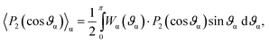 | (1) |
| S = 〈P2(ϑ)〉, and Q = 〈P2(ϑp)〉p, | (2) |
Possessing permanent magnetic moments, the particles respond to an external magnetic field by orienting themselves, thus producing the first statistical moment of the orientation distribution function Wp:
 | (3) |
| M = μNpm, | (4) |
In the general case, both components of a FN might align independently. However, we are interested in the behavior of the FN inside the bulk (the boundaries rest at infinity). So, we assume that the macroscopic orientations of the liquid-crystalline matrix and the particle ensemble are coaxial. Therefore, both the order parameters (2) are defined with respect to the magnetic field direction establishing the symmetry axis of the problem. Note that each of the order parameters might be either positive or negative, the sign corresponding to one of two possible uniaxial structure arrangements: easy-axis or easy-plane. The easy-axis means the orientation along, while the easy-plane corresponds to the orientation across the singled out direction.
3 Mean-field model
In the mean-field approximation we take the free energy density F of the FN in the form similar to those used in ref. 4 and 5. With allowance for a two-component origin of the considered suspension, F is presented as a sum of three contributions referring to the molecular and particle subsystems as such and to their orientational coupling. The contribution, which renders the free energy density of the nematogenic molecules, is well known:6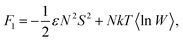 | (5) |
The contribution associated with the embedded magnetic particles is alike that of a paramagnetic gas. For FNs it was first used in ref. 7:
| F2 = −μNpmH + NpkT〈ln Wp〉p, | (6) |
The subsystem coupling in FNs is described by an expression that “crosses” the molecule and particle orientation order parameters. It is presented in the form
| F3 = −εpNNpSQ, | (7) |
The anisotropic surface tension manifests itself in the form of the anchoring effect. Due to this, at any point of the liquid crystal interface with some other substances, gaseous, liquid or solid, the direction of easy (i.e., most energetically favorable) molecular orientation is established. The two main cases of anchoring—perpendicular or parallel to the interface—are termed as homeotropic and planar, respectively. The particular type of orientational anchoring depends on the chemical nature and polarization properties of the nematogenic molecules and also can be modified by an appropriate treatment of the surface.10 The problem of relating the anchoring conditions on the particle surface to the macroscopic coupling constant εp is essential for FNs. Assuming rod-like particles, Brochard and de Gennes7 considered the case of strong anchoring. They showed that, if the local easy direction (of any type) is virtually invariable, then the particles strive to align with the net orientation (director) of the molecular matrix. Therefore, for such systems εp is always positive. Later, the case of a finite (soft) anchoring was investigated by Burylov and Raikher.8 They found that the conclusion of positiveness of εp for rod-like particles holds only for planar surface anchoring. The same particles with homeotropic anchoring settle perpendicular to the director of the bulk nematic thus yielding a negative εp. The authors of ref. 5 considered not only cylindrical (rod-like) particles, as in ref. 7 and 8, but platelets as well. Quite expectedly, it turned out that the platelets with homeotropic anchoring orient themselves perpendicular to the bulk director. For the situation, where the magnetic moment of each platelet lies in its plane, this also implies a negative εp. In view of that, when developing our model, we assume that the ferromagnetic nanoparticles are rod-like and allow the effective εp of a FN to be of either sign. Upon simple redefining of the geometry axis, our formalism equivalently applies to the case of platelets.
Collecting eqn (5)–(7), one obtains the expression for the free energy density of a FN as
 | (8) |
This general formula had been used for description of the phase behavior of FNs in ref. 4. There it was written for the whole sample so that N and Np meant total numbers of molecules (particles). However, the results presented in ref. 4 were not completely correct since the authors failed to properly reformulate expression (8) in terms of volume fractions of the components. An adequate account for the temperature-induced phase transition in a liquid-crystalline suspension of solid non-magnetic particles was given in ref. 5. The free energy density used there follows from eqn (8) at μ = 0. Considerations5 revealed the “dilution” effect, which always reduces the transition temperature.
In eqn (8), it is reasonable to assume, following ref. 4 and 5, that the both non-magnetic interactions are of the same (van der Waals) origin, so that their intensities are proportional:
| εp = ωε. | (9) |
Therefore, ω determines the relative strength of the molecule–particle vs. molecule–molecule orientational couplings.
To proceed with eqn (8) it is convenient to use volume fractions instead of number concentrations. Let ϕ be the volume fraction of the nematogenic molecules and V the molecular volume, then
| N = (1 − ϕ)/V, Np = ϕ/Vp. | (10) |
 | (11) |
Variation of eqn (11) with respect to the molecule (particle) orientation distribution functions yields the equilibrium (Boltzmann) expressions:
 | (12) |
Substituting them in eqn (1) and (3) of the order parameters, we arrive at the expressions
 | (13) |
 | (14) |
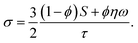
 | (15) |
The factors entering (15) are the dimensionless temperature τ = kT/λ and magnetic field ζ = μH/λ.
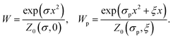
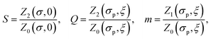
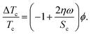
The nonlinear set of eqn (13)–(15) solves easily, if σ is taken as an independent parameter, because all the other variables are single-valued functions of it. After that, one may eliminate σ from any pair of relations and obtain the dependencies of the order parameters on either the temperature τ or the field strength ξ. Functions S(τ) and Q(τ), multivalued as they should be for any first-order phase transition, are shown in Fig. 1 and 2. Vertical lines in these plots correspond to the points τc = kTc/λ of equilibrium transitions determined from equalizing the free energies of the phases; in the physics of liquid crystals the transition temperature Tc is often called the clearing point.
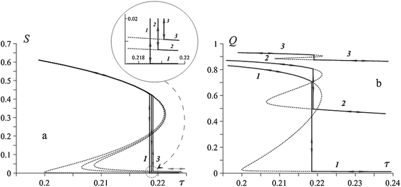 | ||
| Fig. 1 Temperature dependencies of the molecular (S) and particle (Q) order parameters for positive coupling (ω = 2); particle volume fraction ϕ = 0.01 and volume ratio η = 0.06. The field strength is ζ = 0.1 (1), 1 (2), and 5 (3); the parts of the curves corresponding to unstable or metastable states are plotted in dashes, vertical lines mark the equilibrium transition points, their occurrences are detailed in the inset. | ||
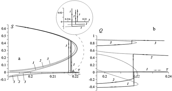 | ||
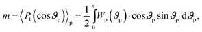
| Fig. 2 Temperature dependencies of the molecular (S) and particle (Q) order parameters for negative coupling (ω = −2); particle volume fraction ϕ = 0.01 and volume ratio η = 0.06. The field strength is ζ = 0.1 (1), 1 (2), and 5 (3); the parts of the curves corresponding to unstable or metastable states are plotted in dashes, vertical lines mark the equilibrium transition points, their occurrences are detailed in the inset; note that in panel (a) the dashed lines, corresponding to ζ = 0.1, lie at the opposite sides of the abscissa axis and do not cross. | ||
4 Paranematic and nematic phases
Let the field be applied to a FN being maintained at a temperature above the clearing point. Had it been a pure nematogen, its phase state would have been isotropic. However, in a FN the field aligns the magnetic particles at any temperature, and the orientational coupling (see eqn (7)) transfers this alignment to the nematogenic molecules. In result, the molecular matrix acquires some macroscopic orientational order. The occurring high-temperature phase is termed paranematic.11 Therefore, in a magnetized FN the isotropic–nematic phase transition is replaced by the paranematic–nematic one.Fig. 1a and b show the phase behavior of a FN in the case of positive coupling (ω > 0), i.e., the easy-axis situation, where parallelicity between the particle axes and nematic director is favored. As mentioned, when the field is on, the high-temperature phase state of the matrix, characterized by the order parameters S, is paranematic. For the employed values of the material parameters, this particle-mediated orientation is rather weak, see the inset of Fig. 1a. With temperature diminution, the transition to the highly ordered (nematic) phase occurs. In Fig. 1a and b this is reflected as vertical ascends from one to another part of the same Z-shaped line. The other branches, obtained from eqn (12)–(14) for the possible orientation states of a FN with positive coupling, are completely unstable and are not shown.
The effect of ordering of the nematogenic matrix on the particles is shown in Fig. 1b. Above the clearing point, the system behaves very much alike a plain magnetic suspension, so that the particles readily align with the field. For example, for ζ = 5, see curve 3, the orientation of the particles is almost saturated yet in the paranematic state. Because of that, at the transition temperature, where the orienting influence of the matrix becomes strong, the increment of Q is small. However, as seen from curves 1 and 2, at weaker fields the orienting effect of the matrix is significant.
In the case of negative coupling (ω < 0) presented in Fig. 2a and b, the situation is different. Under zero field, the particles in such a FN are aligned perpendicular to the director, so that Q at τ → 0 turns to −0.5. At small ζ this arrangement does not change significantly: see line 1 in Fig. 2b, where at the lowest τ = 0.195 the particle order parameter is Q ≃ −0.41, while S in Fig. 2a is positive and large. When heated, both S and Q of a FN with negative ω at first change slowly and gradually. At the transition point, the parameter S falls down, and the particles, being orientationally “liberated”, readily align with the field. In this configuration, the negative coupling forces the molecules of the matrix to orient in the plane perpendicular to the particles and, thus, to the magnetic field, so that the order parameter S becomes negative. In Fig. 2a and b the occurrence of this easy-plane structure means transiting to the other branches of the solution. Note that for the molecules in the system with ω < 0 the transition in the presence of a field always implies the change of sign of S (Fig. 2a). For the particle order parameter (Fig. 2b), the sign changes only at small ζ; however the jump of Q is always directed upward: the more free the particles, the stronger their alignment with the field.
Consider now the same transition but occurring when the system with ω < 0 is cooled down from the paranematic phase (τ > τc). At high temperatures the particles align with the field and are slightly influenced by the matrix. Here, these are the particles, which “prescribe” the orientation arrangement to the matrix, so that the formed paranematic state has the easy-plane structure. However, when approaching the transition point, the energy minimum corresponding to the easy-axis molecular orientation deepens, thus forcing the system to assume this state (positive S) even at the expense of some augmentation of the coupling energy. This scenario is clear from the “trajectories” shown in Fig. 2a and b by arrows. (We remind that in the present consideration the diamagnetic anisotropy of the nematogenic molecules is neglected.)
5 Magnetic field-induced shift of the transition point
As it follows from the very idea of ferronematics7 and numerous experiments, these systems are always dilute solutions of magnetic particles in a nematogen. This justifies treating the effect of the particles on the phase transition temperature in linear approximation with respect to the concentration. The pertinent framework—the thermodynamics of dilute solutions—is well-known, see ref. 12, for example; here we apply it to FNs.The temperature Tc of an equilibrium first-order transition (the clearing point) is defined by a condition under which the free energies of isotropic and anisotropic phases coincide:
| Fan(Tc,ϕ,Wan,Wanp) = Fis(Tc,ϕ,Wis,Wisp), | (16) |
| (λSc2 − ηωλScQc − ημHman − kTc〈ln Wan〉 + ηkTc〈ln Wanp〉p)dϕ + k〈ln Wan〉dTc = (−ημHmis + kTc〈ln Wisp〉p)dϕ, | (17) |
 | (18) |
 | (19) |
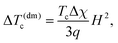
Eqn (19) yields a linear ϕ expression for the transition temperature shift ΔTc. We split the latter in a sum of two contributions as
| ΔTc = ΔTpc + ΔTHc. | (20) |
The first term, ΔTpc, is solely due to the presence of a solid admixture (particles), while ΔTHc emerges only upon switching on the field and depends on its strength. In an explicit form the parts of (20) are
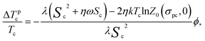 | (21) |
 | (22) |
As a simple test for ΔTpc, one may set in eqn (21)η = ω = 1, i.e., assume that the solvent and admixture are identical. This turns ΔTpc into zero since the numerator of this expression becomes the free energy of a pure nematic at the transition point, see (18).
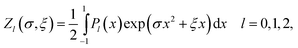
The particle-induced temperature shift rendered by analytical expression (21) is plotted in Fig. 3. This formula reproduces with high accuracy the same dependency obtained numerically by Gorkunov and Osipov.5 As justly remarked in ref. 5, the presence of the particles influences the transition temperature in two opposing ways. On the one hand, as the particles have finite size, there is some excluded volume that entails diminution of Tc(ϕ) in comparison with Tc(0), i.e., the “dilution effect”. On the other hand, as the particles, due to the anchoring conditions on their surfaces, are capable of supporting self-orientation of the matrix, this may enhance Tc(ϕ) with respect to Tc(0). The net result depends on the parameters ω = εp/ε and η = V/Vp, as is shown in Fig. 3. For an illustrative case η = 0.5 considered in ref. 5, the curve ΔTpc crosses the abscissa axis twice, thus proving the above-mentioned decrease/increase of Tc. It is instructive, however, to look at more realistic assumption (particles much larger than molecules). Taking η ∼ 0.06, as in Section 4, one finds that under zero field (i.e., when the particles are in the role of a “passive” admixture), positive values of (Tc(ϕ) − Tc(0)) might occur only at very high absolute values of the coupling parameter, see curve 2 in Fig. 3.
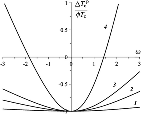 | ||
| Fig. 3 Dependence of the phase transition temperature shift in zero field (ξ = 0) as a function of the subsystem interaction parameter ω; the molecule/particle volume ratio η is 0.01 (1), 0.06 (2), 0.1 (3), and 0.5 (4); note that the results are normalized with respect to the particle volume fraction. | ||
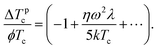
From Fig. 3 one notes that under zero field the matrix–particle coupling of either sign increases Tc at a given ϕ, i.e., aids the FN system to order. This fact becomes explicit, if eqn (21) is to be expanded with respect to small ω:
 | (23) |
The opposite case of large ω also admits analytic representation, which yields
 | (24) |
These formulae explain the difference in steepness between the left (ω < 0) and right (ω > 0) branches of the curves in Fig. 3.
As mentioned above, the value of the macroscopic parameter ω depends on the type of molecule anchoring on the particle surfaces and/or the particle shape. Although any non-zero coupling yields the increase of Tc, the internal structures of FNs with ω's of opposite signs are different. For positive ω the particles are organized in the easy-axis configuration (Q > 0), while for negative ω the particle ensemble assumes the orientational structure of the easy-plane type (Q < 0).
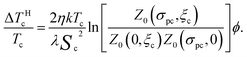
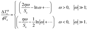
Under a magnetic field, in eqn (20) the field-induced term ΔTHc turns up. In the limiting cases of weak and strong fields, it takes the forms
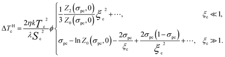 | (25) |
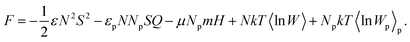
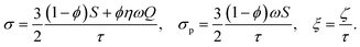
Reference plots for ΔTHc are presented in Fig. 4. The saturation effect in a strong field is well-distinguishable, the limiting value of the corresponding temperature shift being
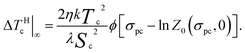 | (26) |
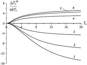 | ||
| Fig. 4 Field dependence of the phase transition temperature shift; parameter ω equals −3 (1), −2 (2), −1 (3), 1 (4), 2 (5), and 3 (6); note that the results are normalized with respect to the particle volume fraction. | ||
As one may see from the definition of the parameter σpc, the sign of the temperature shift coincides with that of the orientation coupling parameter ω. From a qualitative viewpoint, the situation is as follows. The magnetic field always strives to organize the particles into an easy-axis pattern, and for ω > 0 this configuration supports the molecular mean field to establish the uniaxial (nematic) order. Consequently, the contribution from ΔTHc to the transition temperature shift is positive. At negative ω, the field-induced easy-axis alignment of the particles tends to arrange the molecules in the easy-plane way thus impeding the “natural” nematic transition in the matrix; accordingly, in this case ΔTHc is negative, see Fig. 4 and Table 1.
| ζ | ω = 2 | ω = −2 |
|---|---|---|
| τ c(0) = 0.2184839 | τ c(0) = 0.2182901 | |
| [τc(ζ) − τc(0)] × 104 | [τc(ζ) − τc(0)] × 104 | |
| 0.1 | 0.15 | −0.08 |
| 1 | 3.53 | −4.65 |
| 5 | 6.11 | −13.27 |
| ∞ | 7.39 | −15.30 |
Summing up eqn (21) and (26), one gets for the transition temperature shift in a high magnetic field:
 | (27) |
Such a simple form is not occasional. Indeed, in the high field limit the order parameter of the particles saturates (Q = 1), and the set of eqn (21) reduces to a single one
 | (28) |
In this case the particles become a source of a constant effective orienting field f = ϕηλω of quadruple symmetry imposed on the nematic matrix. The free energy of the latter, with allowance for the excluded volume, is
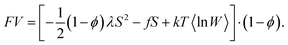 | (29) |
In the linear ϕ approximation, this expression readily yields formula (27) for the temperature shift.
Moreover, expression (29) enables one to analyze the phase transition under the field f without small-parameter assumption. In particular, for the characteristics of the critical end point, i.e., the one where the jump of S turns into zero, for the case ω > 0 one finds
| Tcep = 0.2309λ(1 − ϕ)/k, Scep = 0.2141, fcep/λ = (ϕηω)cep = 0.01045. | (30) |
6 Reference values of the material parameters
The above-described model comprises two orientation fields. One, associated with the nematogenic matrix, is capable of self-ordering and contributes to the free energy proportional to the constant λ. In the limit ϕ = 0 (pure matrix) one recovers the classical Maier–Saupe model. Another field, associated with the particle ensemble, directly responds to the magnetic field and interacts with the matrix the stronger the greater the constant λp = ωλ. In the framework of the Maier–Saupe theory, λ is proportional to Tc, the nematic–isotropic transition temperature: λ ≃ 4.5kTc, see ref. 6, for example. Setting Tc ∼ 300 K, one gets λ ∼ 10−13 erg. To estimate ω, we use the following considerations. Note that the product (1 − ϕ)ωλ is the reference energy to rotate a particle in the nematic phase by about 1 rad with respect to the director. For small concentrations (ϕ ≪ 1), this energy, associated with the non-uniformities of the molecular orientation around a particle equals Kl,7 where K ∼ 3 × 10⁻⁷ dyn6 is the orientation elasticity modulus of the liquid-crystalline phase and l the reference size of a particle. In real ferronematics, the particle size ranges from about micron (needle-like grains13) to tens of nanometers (single particles or their short chain-like aggregates2). For stable systems on the base of ferrofluids, taking l ∼ 5 × 10⁻⁶ cm and substituting chain-like aggregates by solid anisometric objects, one gets ω = Kl/λ ∼ 2–3. However, this value might become smaller in the case of soft (not rigid, as in ref. 7) molecular anchoring, see ref. 8.As far as the magnetic effects are considered, the main controlling parameter is the dimensionless applied field. It enters eqn (13)–(15) either as the temperature-independent quantity ζ = μH/λ or as the temperature-dependent factor ξ = ζ/τ. The magnetic moment of a single ferrite nanoparticle of size 10 nm is about μ ∼ 2 × 10⁻¹⁶ emu and for a chain of a few such particles does not exceed 10−15 emu. Formally, from eqn (13) and after, one finds μ/λ ≃ 10−3 emu erg−1 which means that the parameter ζ reaches unity in a field about 1 kOe. On closer inspection, one notes that the particle magnetic contribution to F may be reduced due to superparamagnetism, the thermofluctuational effect inherent to nanoparticles. In this case the magnetic moment becomes a function of the applied field. The saturation value is recovered, however, under a sufficiently strong field (ξ ≫ 1); the above-given estimates establish that in a FN the superparamagnetism should become negligible at several kOe.
7 Discussion
The presented considerations show that, in principle, each of the above-discussed effects can shift the transition temperature either side with respect to the Tc of a pure nematic. On the other hand, for a particular FN system, where ω and η have fixed values, the net result depends on the strength of the applied field. We note that both contributions to ΔTc given by eqn (21) and (22) are linear in the particle volume fraction ϕ, and due to this their relative magnitudes do not depend on ϕ.Let us compare the field-induced temperature shift in a FN with that obtained in ref. 14 for a pure nematic as due to the diamagnetic anisotropy of its molecules. It is derived in terms of thermodynamic Clausius–Clapeyron equation and gives
 | (31) |
 | (32) |
According to ref. 14, the coefficient dTc/dH2 measured for a typical thermotropic liquid crystal (8CB) is about 2 × 10⁻⁴ mK (kOe)−2. This means that for a shift of the transition temperature by 1 mK, a field about 70 kOe should be applied. In ref. 11 the authors used a more responsive bent-core nematic liquid crystal and a powerful superconducting solenoid. This allowed them to attain a higher field and achieve better accuracy. For their system they obtained dTc/dH2 ≃ 1.5 × 10⁻³ mK (kOe)−2, i.e., an order of magnitude higher than that for 8CB. Substituting in (32)μ = 2 × 10⁻¹⁶ emu (a single 10 nm particle), the reference value Sc = 0.43 and Tc = 300 K, one finds that in a FN the same “magnetothermic” coefficient is dTc/dH2 ≃ 2 × 10³ mK (kOe)−2, i.e., about six orders greater than in a pure nematic. The huge increase of the initial slope of the Tc(H) curve for a FN evidences that even in rather small amounts, the admixed ferroparticles quite strongly affect the isotropic–nematic transition. This comparison is not exhaustive, however. Note that, unlike the diamagnetic orientation, the field-induced alignment of magnetic particles saturates rather fast, see Fig. 4. This means that the temperature shift cannot exceed some limiting value ΔTHc = 2ϕηωTc/Sc ≃ 5ϕηωTc; for the adopted set of material parameters this amounts to ∼1.5 K. The qualitative difference is, however, that this value is obtained in response to a field of a few kOe, while getting the same shift in a pure nematic would require ∼200 kOe. Besides other things, the given estimate justifies neglecting of the diamagnetic contribution of the nematic matrix to the ΔTHc effect as long as moderate fields are considered. We remark also that depending on the anchoring, the transition temperature modulation in a FN might either increase or decrease the clearing point, while the diamagnetic effect always enhances Tc. Moreover, as Fig. 4 points out, under a given field, the absolute change of ΔTHc in a FN with negative coupling is significantly greater than that in a FN with the same, but positive coupling constant. This asymmetry is fundamental. Indeed, as the asymptotic expansion of eqn (26) shows, the leading term in ΔTHc|∞ is proportional to ln ω for positive ω and it is proportional to ω for its negative values.
Finally, we remark that the relations obtained can be directly applied for evaluation of the transition temperature in nematogenic suspensions of ferroelectric nanoparticles. For that, it suffices to just change the magnetic field H and magnetic moments μ for the electric ones, E and p. On doing that, one gets the results, which generalize the recently published ones.9 In that paper the clearing temperature shift in such “ferroelectronematics” is obtained for the case of zero field and only in the limits of strong and weak coupling. For ω ≪ 1, expression (20) of ref. 9, which establishes quadratic dependence of the transition temperature on the coupling parameter, is recovered by our eqn (23). For ω ≫ 1, expression (25) of ref. 9 is valid only for positive coupling and gives just the leading term of the asymptotic expansion. Our eqn (27) in the limit ω ≫ 1 distinguishes the cases of positive and negative coupling and yields the asymptotic form ΔTpc more accurately. Further to that, our eqn (21) and (22) yield the clearing temperature shift in the whole field range, including both limiting cases. When transformed to “ferroelectronematic” notations, the united expression takes the form
 | (33) |
8 Conclusions
A consistent mean-field model is developed that accounts for the field-induced shift of the temperature of the equilibrium isotropic–nematic phase transition (clearing point) in ferronematics: suspensions of ferromagnetic nanoparticles in nematogenic matrices. Depending on the anchoring conditions on the particle surface, the particles might either enhance or decrease the clearing temperature of the suspension. The temperature shift in a ferronematic is evaluated in linear approximation with respect to the particle concentration; for this purpose the thermodynamics of dilute solutions is applied. The field-induced particle-mediated transition temperature modulation is limited due to magnetic saturation of the particles. The expected effect depends on the material parameters of a ferronematic, and the reference value of the transition temperature shift ranges from several tenths to units of Kelvins.We are grateful to P. Kopčanský for drawing this interesting subject to our attention and R. Perzynski for useful discussions. The work was done under auspices of RFBR grant 11-02-96000 and RAS Program 12-P-1018. V.I.S. acknowledges RFBR grant 10-02-96022.
References
- P. Kopčanský, M. Koneracká, M. Timko, I. Potočova, L. Tomčo, N. Tomašovičová, V. Závičová and J. Jadzyn, J. Magn. Magn. Mater., 2006, 300, 75–78 CrossRef CAS.
- N. Tomašovičová, P. Kopčanský, M. Koneracká, L. Tomčo, V. Závičová, M. Timko, N. Éber, K. Fodor-Csorba, T. Tóth-Katona, A. Vajda and J. Jadzyn, J. Phys.: Condens. Matter, 2008, 20, 204123–204125 Search PubMed.
- O. Buluy, S. Nepijko, V. Reshetnyak, E. Ouskova, V. Zadorozhnii, A. Leonhardt, M. Ritschel, G. Schönhense and Y. Reznikov, Soft Matter, 2011, 7, 664–669 Search PubMed.
- R. G. Akhmetzyanov, A. N. Zakhlevnykh and Y. L. Raikher, in Magnetic Properties of Ferrocolloids, ed. M. I. Shliomis, Ural Branch of Acad. Sci. USSR, 1988, pp. 63–74 Search PubMed.
- M. V. Gorkunov and M. A. Osipov, Soft Matter, 2011, 7, 4348–4356 RSC.
- P. G. de Gennes and J. Prost, The Physics of Liquid Crystals, Clarendon Press, Oxford, 1993 Search PubMed.
- F. Brochard and P. G. de Gennes, J. Phys., 1970, 31, 691–708 CAS.
- S. V. Burylov and Y. L. Raikher, Phys. Rev. E: Stat. Phys., Plasmas, Fluids, Relat. Interdiscip. Top., 1994, 50, 358–367 CrossRef CAS.
- L. M. Lopatina and J. V. Selinger, Phys. Rev. E: Stat., Nonlinear, Soft Matter Phys., 2011, 84, 041703–041707 Search PubMed.
- J. Cognard, Alignment of Nematic Liquid Crystals and Their Mixtures, Gordon & Breach, London, 1982 Search PubMed.
- T. Ostapenko, D. B. Wiant, S. N. Sprunt, A. Jákly and J. T. Gleeson, Phys. Rev. Lett., 2008, 101, 247801–247804 Search PubMed.
- L. D. Landau and E. M. Lifshitz, Statistical Physics, Pergamon Press, New York, 3rd edn, 1980 Search PubMed.
- S.-H. Chen and N. M. Amer, Phys. Rev. Lett., 1983, 51, 2298–2301 CrossRef CAS.
- C. Rosenblatt, Phys. Rev. A: At., Mol., Opt. Phys., 1981, 24, 2236–2238 Search PubMed.
| This journal is © The Royal Society of Chemistry 2013 |