Hydrogen bond network topology in liquid water and methanol: a graph theory approach

Abstract

Networks are increasingly recognized as important building blocks of various systems in nature and society. Water is known to possess an extended hydrogen bond network, in which the individual bonds are broken in the sub-picosecond range and still the network structure remains intact. We investigated and compared the topological properties of liquid water and methanol at various temperatures using concepts derived within the framework of graph and network theory (neighbour number and cycle size distribution, the distribution of local cyclic and local bonding coefficients, Laplacian spectra of the network, inverse participation ratio distribution of the eigenvalues and average localization distribution of a node) and compared them to small world and Erdős–Rényi random networks. Various characteristic properties (e.g. the local cyclic and bonding coefficients) of the network in liquid water could be reproduced by small world and/or Erdős–Rényi networks, but the ring size distribution of water is unique and none of the studied graph models could describe it. Using the inverse participation ratio of the Laplacian eigenvectors we characterized the network inhomogeneities found in water and showed that similar phenomena can be observed in Erdős–Rényi and small world graphs. We demonstrated that the topological properties of the hydrogen bond network found in liquid water systematically change with the temperature and that increasing temperature leads to a broader ring size distribution. We applied the studied topological indices to the network of water molecules with four hydrogen bonds, and showed that at low temperature (250 K) these molecules form a percolated or nearly-percolated network, while at ambient or high temperatures only small clusters of four-hydrogen bonded water molecules exist.

---

Introduction

Network structures arise in a wide variety of different contexts, e.g. large communication systems, transportation related logistic problems, social phenomena including networking sites, and in biological systems.¹ Graph and complex network theories allow us to map the large number of interactions into graphs, in which usually just vertices and edges are used as the primary building blocks. Recently, various properties, including the degree distribution, path length, clustering, and the spectral density of the graph, have been introduced for the classification of network structures and to give insight into their interconnectivity and fine structure. Furthermore, the topology of real networks has very often been modeled and compared to the Erdős–Rényi (ER) random graph² or to the more complex Watts and Strogatz small-world (SW)³ graphs or scale free networks. These networks also show the small world³ effect implying that although most nodes are not neighbors of each other, they can still be reached from every other one by a small number of hops or steps.

Hydrogen bonded (HB) networks play an important role in determining the physical properties of many molecular liquids and solids, and play a crucial role in the structure and function of most biomolecules. Among these, water is the most extensively studied material, due to its simple molecular constitution and high biological and chemical importance. The popularity of liquid water as a solvent and many of its unusual properties^4–8 are often attributed to its ability to form a strong and extensive HB network.

Although using the toolbars of complex network theory the structure of networks can be characterized, very little is known about the topologies of HB clusters found in various media. Recently, we investigated the topology of H bonded aggregations in water^9,10 (an example is shown in Fig. 1), water–methanol mixtures,¹¹ formamide and acetic acid,¹² and found that water molecules favour ring structures in contrast to methanol molecules, which prefer to form non-cyclic entities in the bulk phase. We also showed that this behaviour can be interpreted as the signature of the microscopic configurational inhomogeneities in water–methanol mixtures. da Silva et al. arrived at the same conclusion using the spectral density of adjacency matrices and the local clustering coefficients of the network.¹³

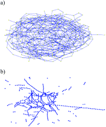Fig. 1 Schematic view of a typical H-bond network in simulated water (a) and methanol (b).

In this article we give a comprehensive overview of the topological properties of the hydrogen bond network in liquid water and methanol focussing mainly on the cyclic topology and the Laplacian spectra. In order to achieve our goal we carried out molecular dynamics simulations on liquid water and methanol, and at the same time generated a representative set of ER and SW graphs. We analyzed the HB network along the MD trajectories and in the generated ER and SW graphs and provide a statistical analysis of the obtained results. We showed that the HB network in water is substantially different from that found in methanol, in agreement with earlier results obtained by different methods, and that various properties of the water network can be described by ER or SW graphs. In the second part of the paper we show how the introduced topological properties can be applied to obtain further information on liquid structure. First, we describe the changes in the topological properties of water as a function of temperature. Then, we discuss how the sub-network of low density patches¹⁴ (network of four-hydrogen bonded water molecules) could be modelled and how their structures change with the temperature. This latter application is especially interesting as it is generally thought that the enhancement of the anomalies of the thermodynamic properties of water in the supercooled region is due to the extensive formation of these hydrogen bonded tetrahedral structures. We anticipate that the method presented here will give insight into the fine-structure of various HB liquids and mixtures. It could also be useful in uncovering how solutes perturb the HB network of aqueous solutions and what kind of changes occur with increasing solute concentration or with changes in temperature. It might also contribute to the exciting field of HB networks formed on the surface of metals,¹⁵ which also play an important role in redox reactions.¹⁶

Methodology

Molecular dynamics (MD) simulations in the NVT ensemble were performed using the DL_POLY 2.20¹⁷ program. Each system (methanol, water) consisted of 2048 molecules in a cubic box at an average temperature of 300 K. Periodic boundary conditions were employed and the Ewald summation was used to handle the long-range Coulombic interactions. The side lengths of the cubes were chosen to correspond to the experimental densities. In the case of water, further simulations were carried out at 250 K and 350 K.

The MD trajectories were generated using the SPC/E¹⁸ and OPLS¹⁹ all site intermolecular potential model for water and methanol, respectively. Although, in recent years a few shortcomings of the SPC/E model have been shown in describing the properties (e.g. phase diagram) of liquid water,²⁰ due to its simplicity it is still commonly used in the literature, and therefore it was used for the present study. The freezing point of water is around 215.5 K when modeled with the SPC/E model under normal conditions,²⁰ for this reason all simulations were carried out above this temperature. Application of the method presented herein to simulations using more accurate water models like TIP4P/2005,²¹ and BK3²² is in progress in our laboratory.

After 600 000 equilibration steps, another 5 000 000 steps were simulated leading to a simulation time of 5.00 ns for each system. Every 0.1 ps a snapshot has been taken and the HB topology has been analyzed. The cumulative data have been used for the statistical analysis of the H bond network topologies. As the best definition of a hydrogen bond has been long debated,²³ here two molecules were regarded as H-bonded if the O⋯H distance was shorter than 2.5 Å, and the interaction energy smaller than −3.0 kcal mol⁻¹. We also tested the effect of using another definition of hydrogen bonds (O⋯H distance shorter than 2.5 Å, and the H–O⋯O angles less than 30°), but as the conclusions based on both definitions qualitatively agreed, only results based upon the first definition will be presented here.

The Erdős–Rényi (ER) random graph model generates a graph that has a fixed number of nodes (equal to the number of molecules in the simulation box, N = 2048 in our case) which are connected randomly by bonds at edges. The average neighbor number of the generated random configurations was set to be 2.95 (ER2.95) or 4 (ER4.0). The first number was chosen as it agrees well with the average coordination number of the molecules in pure water, and the second number (4) was chosen as a representation of four-coordinated molecules and this number can be easily used to generate the small world graphs. In the first case the probability of the occurrence of a bond between two nodes is log(N)/N = p_c, and in this case a random graph almost certainly becomes a percolated network.

In the case of the small-world graph of Strogatz and Watts (SW) we built on the ring lattice C(2048,2). In this case each node is connected to exactly four neighbors. The small world model is then created by moving, with rewiring probabilities of 0.1 (SW1), 0.2 (SW2) and 0.4 (SW3), one end of each bond to a new location chosen uniformly in the ring lattice. In both network models we generated 1000 independent configurations.

Results and discussion

Topological properties of water, methanol, ER and SW graphs

We analyzed the average number of HBs per molecule or node (for simplicity later we will only refer to them as node) and obtained for water 〈k〉 = 2.95, for methanol 〈k〉 = 1.77, for the ER graphs: ER2.95: 〈k〉 = 2.95, ER4.0: 〈k〉 = 4, and 〈k〉 = 4 for all SW graphs independent of the rewiring probability. The value for water l is in accordance with their well-known structure, while the values for the ER and SW graphs originate from the generating algorithm.

Various studies have been published recently on the structure of liquid methanol. Classical simulations suggested that the major cluster present in the liquid is that of branched chains, and that the number of ring structures is negligibly small.^24,25 However, when reverse Monte Carlo simulations were used, the occurrence of rings increased significantly.²⁵ In Table 1, we have collected the statistical properties of liquid methanol obtained from our study. Furthermore, we investigated the effect of branches on the overall liquid structure by deleting the hydrogen bonds to branch points from the structure. Using the latter method, branch points became monomers, thus increasing the f₀ fraction of the clusters, and molecules originally hydrogen bonded to branch points became either end points, increasing the f₁ fraction, or monomers increasing the f₀ fraction. As originally about 2% of molecules belonged to the cluster of monomers, and 7% to the cluster of branch points, the fact that the ratio of the f₀ fraction increased to 14% instead of 9% indicates that in the case of 5% of the chains there is a branch point at the last but one molecule of the chain. The average gel cluster (all clusters with the exception of monomers) size of liquid methanol is 10, which decreases to 4.8 when hydrogen bonds to branch points are deleted from the structure. We performed further analyses of the fraction of bonds between molecules with different numbers of hydrogen bonds (Table S1, ESI†). The data demonstrate that the majority of the molecules are bonded to molecules with two hydrogen bonds, in complete accordance with the previously suggested chain-like structure of liquid methanol.

Table 1 Statistical properties of the molecular clusters in liquid methanol as resulted from molecular dynamics simulation. f_i indicates fraction of molecules with exactly i hydrogen bonds, n_HB is the average number of hydrogen bonds and n_g average gel size

	f 0	f 1	f 2	f 3	n HB	n g
a All molecules were considered. b Wobp stands for without branch points. Methanol molecules with three hydrogen bonds (branch points) were converted to monomers in the statistical analysis. Hydrogen bonds to these molecules were omitted.
All^a	0.02	0.246	0.653	0.072	1.77	10.68
Wobp^b	0.148	0.350	0.501	—	1.35	4.82

---

The fraction of nodes with exactly j bonds is shown in Fig. 2. The shape and the width of the bonded neighbor number distributions exhibit significant differences in the studied systems. The distribution function of methanol is narrow, and most molecules have only two bonded neighbors in accordance with the chain-like structure suggested earlier. This distribution is best modelled by the SW1 graph, but it is centered on k = 4. The distribution function of SW graphs becomes wider and flatter with increasing rewiring probability, but maintains their peak position at k = 4. The ER network distributions have long tails indicating that a small number of nodes have many bonded neighbors in contrast to the SW networks or to physically existing water and methanol systems where steric constraints impede the formation of such nodes. There is an apparent similarity between the degree distribution of water and SW3, with the main difference being a small shift of the center of the peak.

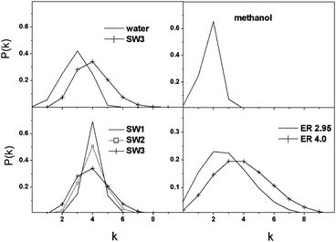Fig. 2 Fraction of bonded neighbours (P(k)) as a function of the number of HB neighbours (k).

Earlier, we have shown that liquid water contains several cyclic structures.⁹ In order to estimate the cycle to open chain ratio in the systems, ring search algorithms²⁶ were used to find primitive rings, which cannot be decomposed into smaller rings, of oxygen atoms and hydrogen bonds.

The ring size distribution of methanol or water has a well-defined maximum around 5 and 6, and is substantially different from that of the graph models (see Fig. 3). In the case of methanol this number agrees with the methanol hexamer structures observed on the surface of Au(111).²⁷ However, in methanol we found approximately three orders of magnitude smaller number of cyclic entities than in water or in the graph models, which has to be taken into account when the data are interpreted for methanol. A further breakdown of the ring-size distribution of methanol shows that 97.7% of the molecules are found in non-cyclic structural elements (as monomers or members of a linear chain), 2.3% belong to primitive rings, and only about 0.01% of the molecules belong to composite rings, indicating a statistically insignificant contribution to the overall structure. A molecule is said to be part of a composite ring, if it belongs to two or more primitive rings. The obtained values are in good agreement with the results of earlier classical simulations,^24,25 and with the structure that can be envisaged based upon Fig. 1.

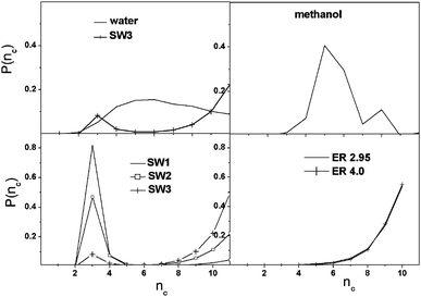Fig. 3 Size distribution of cyclic entities as a function of n_c, number of nodes forming the cycle.

In SW networks many small-sized structural entities exist compared to the other systems, but their number decreases with increasing rewiring probability giving place to the formation of larger rings. The ring size of 3 corresponds to a clique, which is a maximal complete subgraph of three or more nodes. In the case of water we did not find such a motif, which is probably due to the steric constraint that would destabilize such a small ring. The lack of 6-membered rings in all SW graphs is in sharp contrast to the water and methanol systems. The ER networks contain only rings with more than 5 nodes in considerable amounts, and the probability of the occurrence of the rings rises sharply with the ring size. Therefore it seems that the network structure of water is quite peculiar that is not imitated by the graph models used in this study.

The local cyclic coefficient (r_ci) of a node i (eqn (1)) and the local bonding coefficient of a bond (r_b, eqn (2)) characterize the degree of circulation in complex networks:²⁸

where k_i is the number of bonded neighbors of the ith node and S_lmi is the smallest sized closest path that passes through i and its two neighbor sites, l and m, and N_c is the number of primitive rings, which contain the bond, and n_c is the size of the cycles. From these, the value of r_ci can vary from zero, when the network has perfect tree-like structure, to the maximum of 1/3. Larger values of r_ci imply more rings, and r_ci becomes equal to 1/3 when all the neighbor pairs of the node have direct links to each other. The value of r_b is proportional to 1/N_c and if there are no rings in the system, the value of r_b diverges to infinity. Therefore, in eqn (2) we investigated only those edges (bonds), which are incorporated at least in one cyclic structure. The smallest cyclic size was 3 (n_c). If there are only three-membered cycles in the system, the value of r_b reaches its maximum, it is equal to 1/3. However, when there are larger rings in the system, the value of r_b decreases, similarly to the value of r_ci. The probability distribution of r_c (Fig. 4) and r_b (Fig. S1 in the ESI†) exhibits similar features. The P(r_c) distribution of ER and water networks shows Poisson-like shapes with a peak around 0.10 and 0.12, respectively. The distribution of the SW1 network has a strong peak at 0.21, due to the presence of many small, three-membered rings discussed above. With increasing rewiring probability the shape of the distribution function changes significantly indicating the formation of new, larger structural elements, and in the case of SW3 a larger wide peak appears between 0.1–0.15 similar to that found in water.

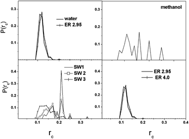Fig. 4 Histograms of the local cyclic coefficients (r_c).

The structure of the networks can be completely described by the associated adjacency (A), combinatorial Laplace (L) or normalized Laplace matrices (L³).^29–32 The adjacency matrix is defined as A_ij = 1 if a bond exists between the nodes i and j and A_ij = 0 otherwise. The combinatorial Laplace matrix is defined according to eqn (3) as:

L_ij = k_iδ_ij − A_ij (3)

where k_i is the number of bonded neighbors of node i.

The spectrum of a graph is the set of eigenvalues of its corresponding matrices (A, L). Properties of the eigenvalues and the eigenvectors of these matrices are characteristic of the network structure. The solutions to diffusion and flow problems related to liquids forming complex networks (spreading diseases, random walks) were earlier shown to be closely related to the combinatorial Laplacian spectra.²⁹

The Laplacian spectra of water, SW and ER networks are continuous like (see Fig. S2, ESI†), but that of methanol has several well-defined peaks (λ = 1, 1.5, 2, 3…). Laplacian spectra of these continuous like graphs are skewed with the main bulk pointing towards the small eigenvalues. It has already been shown that with increasing average neighbor number (ER graph) or rewiring probability (SW graph) the bulk part of the spectrum becomes bell-shaped.³¹ In the uncorrelated graph the spectral density converges to a semicircular distribution as described by Wigner's-law.

The smallest positive eigenvalue of a Laplacian or Fiedler eigenvalue³¹ is a measure of how strongly the network is connected. In the case of water (see Fig. 5) we detected a peak at 0.05 indicating the existence of strong network communities. An increase in the clustering coefficients of ER graphs results in a group of eigenvalues close to 0.0.

Fig. 5 Spectral density of the Laplace matrix at small eigenvalues.

Another prominent feature of the eigenvalue problem of the L matrices is revealed by the structure and localization of the components of the eigenvectors. We can characterize these eigenvectors (λ_j) using the inverse participation ratio (I) as

where V_ji is the ith element of jth eigenvector. I ranges from the minimal value of 1/N corresponding to the eigenvector distributed equally on all nodes to a maximum of 1 for a vector with only one nonzero component.^29c,32 Similarly, we can characterize the average localization of the ith node aswhere the summation goes over the ith components of the eigenvalues. It has to be noted here that I_j should not be mixed up with D_i in eqn (5). The index i stands for a node and j stands for the eigenvectors of Laplacian. Hence I_j is characterized by the localization of the j eigenvectors and D_i is characterized by the i nodes.

Fig. 6 depicts the localization of the eigenvectors and implies that the degree of localization is significantly higher at larger eigenvalues in the case of ER, SW and water networks, while remains almost constant for methanol. The large peaks occurring for water at eigenvalues 1, 2 and 3 indicate the presence of monomers, dimers and trimers.

Fig. 6 Inverse participation ratio of Laplacian eigenvectors plotted against the corresponding eigenvalues.

The localization function of the nodes changes significantly with the neighbor number, and for low neighbor numbers it has a power-tail like distribution for water, ER and SW graphs implying the homogeneity of the system (see Fig. 7). As the neighbor number increases the shape of the P(I_d) function changes and becomes tree-like indicating inhomogeneities. The most eye-catching change occurs at I_d = 5 for water, I_d = 6–7 for the ER2.95 and SW3 graphs, while it was present at almost all I_d values for methanol. From the tree-like structure of methanol we can clearly detect the existence of the different localization of 1, 2 or 3 H-bonded methanol molecules. This result is consistent with the known differences between the network structure of water and methanol, and it also shows that from this aspect ER and SW graphs can be tuned to behave like water or methanol.

Fig. 7 Histograms of the average localization of a node decomposed according to the neighboring number. Symbols corresponding to nodes with various neighbor numbers are shown in the figure of methanol, but for all systems the same symbols are used.

Changes in the topological properties of water as a function of temperature

Our findings on the topological properties of water, methanol and small world graphs suggest that these properties may capture some of the intrinsic properties of liquid structure. For this reason, we decided to apply them to liquid water at various temperatures (250 K, 300 K and 350 K) and investigate whether any systematic differences could be detected in the HB structure of water at low, ambient and high temperatures.

First, we have analyzed the intermolecular pair correlation function of the O⋯O distances (see Fig. 8). With increasing temperature we observe that (1) the second peak at 4.8 Å disappears and (2) the minimum (at the O⋯O distance of 3.4 Å) is filled up. Both of these phenomena indicate the disappearance of the second solvation shell of water at higher temperatures, which is also due to the appearance of interstitial water molecules, which, although they are close to the central water molecule, do not form hydrogen bonds with it. Their appearance may also contribute to the decrease of the density of water.

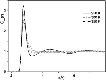Fig. 8 O⋯O partial radial distribution functions of water at various temperatures (in K).

The collected values in Table 2 show that the average hydrogen bond number (〈k〉 and 〈k₄〉) and the number of cycles (N_c and N_c,4) significantly decrease with increasing temperature.

Table 2 Average neighbor number (〈k〉), number of primitive rings (N_c) in water at various temperatures. Average neighbor number (〈k₄〉), fraction of water molecules with four hydrogen bonded neighbors (F₄), number of primitive rings (N_c,4) in the low density patch of water at various temperatures

T (K)	〈k〉	N c	〈k4〉	F 4	N c,4
250	3.18	2978.1	1.41	0.566	309.2
300	2.95	2197.3	0.85	0.423	81.9
350	2.68	1530.1	0.52	0.323	25.8

---

Analysis of the changes in the cycle size distribution of water as a function of temperature (Fig. 9a) also indicates the disappearance of the second solvation shell. While at low temperature 5 and 6 membered ring structures dominate the network structure, at higher temperatures the contribution of larger rings to the liquid structure is also significant. The same conclusion can also be drawn from Fig. S3 (ESI†), where the distribution of local cyclic coefficients (r_ci) is shown. As mentioned above, the value of r_ci = 0 implies a perfect tree-like structure of the network, while the maximum value of r_ci is 1/3. We can observe that with increasing temperature the distribution function becomes wider while the peak height of the largest peak decreases, indicating that the uniformity of the network structure observed at low temperature (i.e. that 5 and 6 membered rings dominate the network structure as concluded from Fig. 9a) changes as the temperature increases and new topological elements with larger rings make the network structure more versatile.

Fig. 9 (a) Cycle size distribution in water as a function of temperature. (b) Cycle size distribution of the low density patch (neighbouring hydrogen bond number (k) is 4).

Finally, we compared the spectral densities of the Laplace matrices as a function of temperature (Fig. 10a). Significant changes in the spectra occur primarily at low λ values. On the one hand the first peak gets closer to 0, and on the other hand the second peak becomes much less pronounced as the temperature increases (see the inset in Fig. 10a). These imply that fundamental changes occur in the network structure as the temperature increases. Furthermore, the increase of the peaks at λ = 1 and 2 also indicates that there are more and more monomers and dimers in the system as the temperature increases in accordance with earlier results indicating the increasing presence of interstitial water molecules.

Fig. 10 (a) Spectral density of Laplace matrix in water at different temperatures (in K). The inset shows a section of the same spectra at small eigenvalues. (b) Spectral density of Laplace matrix of water for the low density patches at different temperatures (in K).

Topological properties of water molecules with four hydrogen bonds

Stanley et al. suggested that water molecules with four hydrogen bonds form small ramified patches whose density is lower than that of water (low density patches).^14,33,34 As these tetrahedral structures are thought to play a major role in the enhancement of the anomalies in the thermodynamic properties of water in the supercooled state we decided to compare the topological properties of the low density patches at various temperatures. We used the same procedure presented above, but the adjacency matrix of the low density patches was defined as A_ij,4 = 1 if a bond exists between the nodes i and j, and both k_i = 4 and k_j = 4, otherwise A_ij = 0.

Our first observation is that for the low density patches the average hydrogen bond number (〈k₄〉) significantly decreases with increasing temperature similarly to the trend observed for the whole ensemble of water molecules. The fraction of four bonded water molecules (F₄) shows the same effect, while the four bonded water molecules form about one order of magnitude less cycles at 350 K than at 250 K (Table 2). The average hydrogen bond number (〈k₄〉) at 250 K is 1.41, which is very close to the percolation limit suggested for (k = 1.53) ST2 water,³³ and may indicate that in the low temperature region the low density patches form a percolated or nearly percolated network. In order to investigate this possibility in more detail, we looked at the cluster size distribution of the low density patches at various temperatures (Fig. 11). Percolation can be monitored by the comparison of the calculated cluster size distribution function of the present system with that obtained for a random percolation on a 3D cubic lattice³⁵ with P(n_c) = n_c^−2.19. In percolating systems the cluster size distribution exceeds this predicted function at large cluster size values. From Fig. 11 we can conclude that at 350 K there are many, very small clusters, and as the temperature decreases the size of the clusters increases. At 300 K and 350 K the low density patches of water do not form percolating networks. At 250 K we find large clusters with several hundreds of members showing the percolation of the network. These findings are visually depicted in Fig. 12, where snapshots of the network structure of the low-density patches are shown at various temperatures.

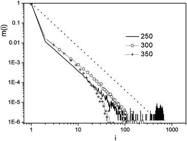Fig. 11 Cluster size distribution in liquid water at various temperatures (in K) for low density patches. The dotted line represents the random percolation network P(n_c) = n_c^−2.19.

Fig. 12 Selected examples of the low density patches found in water at 250 K (a) and 350 K (b). HB network of water at ambient temperature is depicted in Fig. 1 for comparison.

We compared the cycle size distribution of the low density patches (Fig. 9b) to the overall HB network in water. At 350 K four-membered cycles dominate the network structure of the low-density patches, but with decreasing temperature cycle sizes of mainly 5 (and 6) become dominant. This observation is interesting because it shows that at 250 K the low density patches begin to have a similar cycle size distribution that is characteristic of the overall HB structure of water at ambient temperatures.

Finally, we studied the Laplace spectra of the low density patches (Fig. 10b). At 350 K there are many more peaks close to zero than at 250 K, which, as mentioned above, indicate the presence of disconnected components (i.e. in our case clusters). This result is in very good agreement with the conclusions drawn from Fig. 11 or 12: at 350 K there are many small clusters of four-hydrogen bonded molecules, which do not form a single percolated network. The network structure continuously changes as the temperature decreases and at 250 K, there are more molecules with 4-hydrogen bonds and they form a percolated network.

Conclusions

We studied and compared the topological properties of liquid water, methanol, small world and Erdős–Rényi random networks. We used various descriptors to characterize them: the neighbour number distribution, cycle size distribution, the distribution of local cyclic and local bonding coefficients, Laplacian spectra of the network, inverse participation ratio distribution of the eigenvalues and average localization distribution of a node. We demonstrated that several properties (e.g. the local cyclic and bonding coefficients) of the network in water resemble the SW and/or ER networks. However, our results also indicate that the ring size distribution of water is very characteristic and none of the studied graph models could be used to describe it. Using the inverse participation ratio of the Laplacian eigenvectors, we found that network inhomogeneities occur in water at neighboring numbers larger than 4 and showed that similar phenomena can be observed in ER and SW graphs.

We also tested the predicting power of the topological properties in two applications. First, we studied the temperature dependence of the topological properties of the hydrogen bond network in liquid water and showed that (1) at low temperatures 5 and 6 membered rings dominate the network structure of water and (2) with increasing temperature the topological properties indicate the disappearance of the second solvation shell of water and the appearance of larger ring structures together with the increasing presence of interstitial water molecules. The latter findings are in accordance with previous experimental and theoretical findings. We also investigated the network structure of low density patches (of water molecules with four hydrogen bonds) at low temperature (250 K) and found that these patches form an extended, percolated network, that is not present at 300 K or 350 K.

We hope that our results could open up new ways for the application of the tools of network theory to HB networks and that they could contribute to our understanding of the static and dynamical network structure of hydrogen bonded substances. They could also provide a means for the study of inhomogeneities in the hydrogen bond network of aqueous solutions and mixtures or even on metal surfaces playing a role in redox reactions.

Acknowledgements

The authors thank Hungarian OTKA for grant number: K108721. J.O. is thankful for the financial support of the European Commission under a Marie Curie Fellowship (project “Oestrometab”) and of the New Széchenyi Plan (TÁMOP-4.2.2/B-10/1-2010-0009). K.H. acknowledges support from the Swedish national strategic research program in e-science eSSENCE. We are grateful to the Hungarian NIIF computer resource centre and Juellich Supercomputer Center.

Notes and references

1. R. Albert and A.-L. Barabási, Rev. Mod. Phys., 2002, 74, 47; S. N. Dorogovtsev and F. F. Mendes, Adv. Phys., 2002, 51, 1079; H. Jeong, S. Mason, R. Albert, A.-L. Barabási and Z. N. Oltvai, Nature, 2001, 411, 41; A.-L. Barabási and R. Albert, Science, 1999, 286, 509; M. E. J. Newmann, S. H. Strogatz and D. J. Watts, Phys. Rev. E: Stat., Nonlinear, Soft Matter Phys., 2001, 64, 026118; S. Boccaletti, V. Latora, Y. Moreno, M. Chavez and D.-U. Hwang, Phys. Rep., 2006, 424, 175; J. Onnela, J. Saramäki, J. Hyvönen, G. Szabo, M. A. de Menezes, K. Kaski, A.-L. Barabási and J. Kertesz, New J. Phys., 2007, 9, 179.
2. P. Erdős and A. Rényi, Publ. Math., 1959, 6, 290; P. Erdős and A. Rényi, Acta Math. Acad. Sci. Hung., 1961, 12, 261; B. Bollobás, Random graph, Academic London, 1985.
3. D. J. Watts and S. H. Strogatz, Nature, 1999, 393, 440.
4. Homepage of M. Chaplin, http://www.lsbu.ac.uk/water/.
5. F. Sciortiono and S. L. Fornili, J. Chem. Phys., 1989, 90, 2786; P. Kumar, G. Franzese, S. V. Buldyrev and H. E. Stanley, Phys. Rev. E: Stat., Nonlinear, Soft Matter Phys., 2006, 73, 041505; H. E. Stanley, Z. Phys. Chem., 2009, 223, 939; J. Holzmann, A. Appelhagen and R. Ludwig, Z. Phys. Chem., 2009, 223, 1001; D. A. Schmidt and K. Miki, J. Phys. Chem. A, 2007, 111, 10119; D. A. Schmidt and K. Miki, ChemPhysChem, 2008, 9, 1914.
6. A. Luzar, Chem. Phys., 2000, 258, 267; A. Luzar and D. Chandler, Nature, 1996, 379, 55.
7. J. R. Errington and P. G. Debenedetti, Nature, 2001, 409, 318; J. R. Errington, P. G. Debenedetti and S. Torquato, Phys. Rev. Lett., 2002, 89, 215503.
8. M. Matsumoto, A. Baba and I. Ohmine, J. Chem. Phys., 2007, 127, 134504; M. Matsumoto, AIP Conf. Proc., 2008, 982, 21854.
9. I. Bakó, T. Megyes, S. Bálint and V. Chihaia, Phys. Chem. Chem. Phys., 2008, 32, 5004.
10. G. Pálinkás and I. Bakó, Z. Naturforsch., A: Phys. Sci., 1990, 46, 95.
11. I. Bako, T. Megyes, S. Bálint, T. Grósz and M.-C. Bellisent-Funel, J. Chem. Phys., 2010, 132, 014506.
12. T. Megyes, S. Bálint, T. Grósz, L. Kótai and I. Bakó, J. Mol. Liq., 2008, 143, 23.
13. J. A. B. da Silva, F. G. B. Moreira, V. M. L. dos Santos and R. L. Longo, Phys. Chem. Chem. Phys., 2011, 13, 6452; A. B. da Silva, F. G. B. Moreira, V. M. L. dos Santos and R. L. Longo, Phys. Chem. Chem. Phys., 2011, 13, 593; V. M. L. dos Santos, F. G. B. Moreira and R. L. Longo, Chem. Phys. Lett., 2004, 390, 157.
14. A. Geiger and H. E. Stanley, Phys. Rev. Lett., 1982, 49, 1749.
15. M. Mura, F. Silly, V. Burlakov, M. R. Castell, G. Andrew, D. Briggs and L. N. Kantorovich, Phys. Rev. Lett., 2012, 108, 176103.
16. M. Forster, R. Raval, A. Hodgson, J. Carrasco and A. Michaelides, Phys. Rev. Lett., 2011, 106, 046103.
17. DL_POLY is a package of molecular simulation routines written by W. Smith and T. Forester, CCLRC, Daresbury Laboratory, Daresbury, Nr. Warrington, 1996.
18. H. J. C. Berendsen, J. R. Grigera and T. P. Straatsma, J. Phys. Chem., 1987, 91, 6269.
19. W. L. Jorgensen, D. S. Maxwell and J. Tirado-Rives, J. Am. Chem. Soc., 1996, 118, 11225; W. L. Jorgensen, Encyclopedia of Computational Chemistry, Wiley, New York, 1998, vol. 3, Chap. OPLS Force Fields.
20. P. T. Kiss and A. Baranyai, J. Chem. Phys., 2011, 134, 054106.
21. J. L. F. Abascal and C. Vega, J. Chem. Phys., 2005, 123, 234505.
22. P. T. Kiss and A. Baranyai, J. Chem. Phys., 2013, 138, 204507.
23. R. Kumar, J. R. Schmidt and J. L. Skinner, J. Chem. Phys., 2007, 126, 204107 and references therein.
24. P. Gómez-Álvarez, L. Romaní and D. González-Salgado, J. Chem. Phys., 2013, 138, 044509; J. Lehota, M. Hakala and K. Hamalainen, J. Phys. Chem. B, 2010, 114, 6426.
25. A. Vrhovsek, O. Gereben, A. Jamnik and L. Pusztai, J. Phys. Chem. B, 2011, 115, 13473.
26. V. Chihaia, S. Adams and W. F. Kuhs, Chem. Phys., 2005, 317, 208.
27. J. L. Timothy, J. Carrasco, A. E. Baber, A. Michaelides, E. Charles and H. Sykes, Phys. Rev. Lett., 2011, 107, 256101.
28. H.-J. Kim and J.-M. Kim, Phys. Rev. E: Stat., Nonlinear, Soft Matter Phys., 2005, 72, 036109; H.-J. Kim and Y.-M. Choi, J. Phys. Soc. Jpn., 2007, 76, 044801.
29. (a) S. N. Dorogovtsev, A. V. Goltsev, J. F. F. Mendes and A. N. Samuhkin, Phys. Rev. E: Stat., Nonlinear, Soft Matter Phys., 2003, 68, 046109; (b) I. J. Farkas, I. Derényi, A.-L. Barabási and T. Vicsek, Phys. Rev. E: Stat., Nonlinear, Soft Matter Phys., 2001, 64, 026704; (c) P. N. Mcgraw and M. Menzinger, Phys. Rev. E: Stat., Nonlinear, Soft Matter Phys., 2008, 77, 031102; (d) F. Chung, L. Liu and V. Vu, Proc. Natl. Acad. Sci. U. S. A., 2003, 100, 6313; (e) A. N. Samuhkin, S. N. Dorogovtsev and J. F. F. Mendes, Phys. Rev. E: Stat., Nonlinear, Soft Matter Phys., 2008, 77, 036115; (f) E. P. Wigner, Ann. Math., 1955, 62, 548; (g) E. P. Wigner, Ann. Math., 1957, 65, 203; (h) E. P. Wigner, Ann. Math., 1958, 67, 325.
30. M. Barahona and L. M. Pecora, Phys. Rev. Lett., 2002, 89, 054101; R. Kuhn and J. van Mourik, J. Phys. A: Math. Theor., 2011, 44, 165205; X. Ma, L. Huang, Y. C. Lai and Z. Zheng, Phys. Rev. E: Stat., Nonlinear, Soft Matter Phys., 2009, 79, 056106.
31. M. Fiedler, Czech. Math. J., 1973, 23, 298.
32. M. Mitrowic and B. Tadic, Phys. Rev. E: Stat., Nonlinear, Soft Matter Phys., 2009, 80, 026123.
33. R. L. Blumberg, H. E. Stanley, A. Geiger and P. Mausbach, J. Chem. Phys., 1984, 80, 5230.
34. H. E. Stanley and J. Teixeira, J. Chem. Phys., 1980, 73, 3404.
35. A. Oleinikova, I. Brovchenko, A. Geiger and B. Guillot, J. Chem. Phys., 2002, 117, 3296; N. Jan, Physica A, 1999, 266, 72.

---

Footnote

† Electronic supplementary information (ESI) available: Table S1: the fraction of bonds between molecules with different numbers of hydrogen bonds; Fig. S1: the histogram of the local bonding coefficient (r_b) for the investigated systems; Fig. S2: spectral density of the Laplace matrix for the investigated systems; Fig. S3: the histogram of the local cyclic coefficient (r_c) for the low-density patch of water at various temperatures (in K). See DOI: 10.1039/c3cp52271g

---