Characteristics of surface ozone at an urban site of Xi'an in Northwest China

Abstract

Surface ozone concentrations in Xi'an, China were monitored from March 23, 2008 to January 12, 2009 using the Model ML/EC9810 ozone analyzer. The daily average O₃ ranged from <1 ppb to 64.2 ppbv with an annual average of 16.0 ppbv. The seasonal average of O₃ in summer (32.5 ppbv) was more than 10 times higher than that in winter (3.0 ppbv). A significant positive correlation was found between ozone concentration and ambient temperature, indicating that the intensity of solar radiation was one of the several major factors controlling surface ozone production. Using the NOAA HYSPLIT 4 trajectory model, the three longest O₃ pollution episodes were found to be associated with the high biogenic volatile organic carbon (BVOC) emissions from the vegetation of Qinling Mountains. No significant weekday and weekend difference in O₃ levels was detected due to the non-significant change in NO_x emissions. O₃ depletion by NO emission directly emitted from vehicles, low oxygenated VOC concentrations, and low-level solar radiation caused by high aerosol loading all contributed to the low levels of O₃ found in Xi'an compared to other cities and rural areas.

---

Environmental impact

This manuscript investigated the characteristics of surface ozone over Xi'an, the largest city in semi-arid areas in northwestern China. The highest O₃ levels appeared in early afternoon and in hot seasons while the lowest O₃ levels appeared in early morning and in cold seasons. The mean O₃ levels in Xi'an were in a similar order of magnitude to several other Chinese cities in southern China, although lower than many cities outside China. The longest O₃ episodes were found to be caused by air masses containing high biogenic VOC emissions originating from vegetation of the Qinling Mountains. No significant weekday and weekend differences in O₃ levels were detected due to the non-significant change in NO_x emissions.

1. Introduction

Ozone has attracted extensive attention due to its important roles in air quality, climate change and ecosystem health.^1–4 O₃ is a critical photochemical oxidant in the troposphere and affects atmospheric chemistry and air quality. Excessive surface O₃ could cause adverse effects to human health, vegetation and materials.^5–7 O₃ is also one of several important greenhouse gases directly contributing to climate change due to its absorption of the Earth's infrared radiation at 9.6 μm. Exposure to harmful O₃ concentrations has been observed in ambient air in many places around the world.^8,9 Hence, it is essential to evaluate the O₃ levels in urban and rural areas in order to improve air quality and to protect the earth creatures from such adverse effects.

Temporal variations of surface O₃ and related meteorological factors have been extensively studied around the world.^3,10–13 These studies have comprehensively analyzed the factors and processes affecting O₃ formation, accumulation, transport, and deposition. Periods of high O₃ concentrations are often associated with intense solar radiation, high temperature, stagnant air, and minimum rainfall; all of these are favorable for the photochemical production of ozone and the accumulation of pollutants in the atmospheric boundary layer. High ozone concentrations might be registered within the metropolis and downwind locations due to high O₃-precursor emissions in urban areas.^14,15 These precursors may also be transported over long distances, resulting in ozone formation far from the sources under the influence of meteorological conditions.

Studies on the characteristics of ozone and its precursors in China were mostly conducted in the three developed regions: Pearl River Delta Region (PRD), Yangtze Delta region (YDR), and Beijing–Tianjin Region.^7,16–23 These studies have provided the spatial and seasonal distributions of ozone concentrations in these regions of China. For example, the highest O₃ often appeared downwind of the developed regions and a clear gradient of O₃ was found from the southeast to the northeast. Higher O₃ levels were commonly observed in summer in these areas. However, in some cities located at the lower latitudes in south China, such as Hong Kong and Guangzhou, low ozone levels have also been observed in summer due to the strong influence by summer monsoons.^17,24

To our knowledge, no study on ambient O₃ has been conducted in urban regions in the northwest of China. Although these areas belong to the developing regions in China in comparison with PRD, YDR, and Beijing–Tianjin Region, economic growth in these areas has been very fast since the establishment of the ‘West region Development Strategy’ by the Chinese Central Government in recent years. Xi'an, the capital city of Shaanxi province in northeast China, is located in the Guanzhong Plain area with a topographic basin surrounded by the Qinling Mountains to the south and the Loess Plateau to the north (Fig. 1). Qinling Mountain is 1500 km in length and 300 km in width and is fully covered with lush vegetation in summer. The city Xi'an is just 20 km north of the mountain. The population of Xi'an was 8.47 million at the end of 2010. As the largest city in northwestern China, Xi'an faces rapid urban expansion and development. The increasing anthropogenic emissions have already led to high levels of airborne particulate matters in the past few years.^25–30 Coal remains as the main fuel for energy production in Xi'an and other Chinese cities and contributes to the high pollution levels. In addition, the number of motor vehicles in Xi'an has grown rapidly, increasing from ∼180 000 in 1997 to ∼1 200 000 in 2010. In this study, one year of O₃ data was obtained at an urban site in Xi'an. The purpose of the present study is to assess the current O₃ levels in Xi'an and to investigate factors controlling O₃ level. The results are expected to be helpful for making policy decisions related to improving air quality.

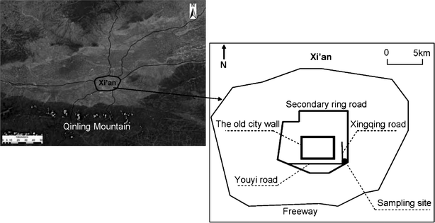Fig. 1 Location of the sampling site.

2. Methods

2.1. O₃ observation

A UV photometric O₃ analyzer (Model ML/EC9810, Ecotech Pty Ltd, Australia) was used to continuously monitor ground-level ozone every 5 min at Xi'an station from March 23, 2008 to January 12, 2009. The monitoring site for O₃ observation (34°15′N, 108°56′E, 400 m above sea level) was located on the roof of a 15 m high building inside Xi'an Jiaotong University (Fig. 1). North and east of the sampling site were residential areas and the campus of Xi'an Jiaotong University, while to the south and west were the South Second Ring and Xingqin Roads, where the traffic was always heavy. The sampling site was considered to be representative of the urban characteristics in Xi'an and thus was suitable for studying the urban surface-level O₃.

Zero checks were performed every day by automatically injecting charcoal-scrubbed air. Almost one year’s worth of monitored ozone concentration data (except the periods of network maintenance and upgrading) at the above mentioned site were used to analyze the characteristics of ground-level ozone in Xi'an. There were limited numbers of measurements in August, as the ozone analyzer was undergoing maintenance.

2.2. Meteorological data, NO₂ concentration, and back trajectory analysis

During the sampling periods, hourly meteorological data, including ambient temperature, wind speed, wind direction, and rainfall were recorded by the Shaanxi meteorological agency. The meteorological station is located in the northern part of Xi'an city, nearly 6 km away from our sampling site.

The air pollution indices (APIs) for NO₂ at Xingqin road station (which is nearly 0.5 km to the ozone observation site) were obtained from the Xi'an Environmental Protection Bureau and converted to concentrations using the following equation:

C = C_low + [(I − I_low)/(I_high − I_low)] × (C_high − C_low) (1)

where C is the concentration (mg m⁻³) and I is the unitless API value. I_high and I_low, are the two values most approaching the value I in the API graded limited-value table;³¹C_high and C_low represent the concentrations corresponding to I_high and I_low, respectively.

Air mass back-trajectory is a useful tool to identify the possible source regions and transport pathways of air pollutions. In this study, 24 h air mass back-trajectory was calculated using the NOAA HYSPLIT 4 trajectory model to trace the source and transport pathways of O₃ or its precursors.

3. Results and discussion

Daily and hourly average O₃ concentrations were analyzed to first obtain its seasonal and diurnal patterns (3.1) and the effects of meteorological conditions on O₃ formation (3.2); O₃ episodes were then explored using air-mass back trajectories (3.3); potential weekday and weekend differences were briefly discussed (3.4); and a comparison with O₃ levels in other urban and rural sites around the world was provided at the end of this section.

3.1. Seasonal and diurnal patterns of O₃ levels

Time series of daily average O₃ concentrations during the monitoring period is shown in Fig. 2. The daily average O₃ concentration ranged from <1 ppbv to 64.2 ppbv, with an annual average of 16.0 ppbv. Daily O₃ levels had a clear seasonal variation pattern, with the average O₃ level in summer tenfold higher than that in winter. The highest daily average reached 64.2 ppbv on June 5, which also corresponded to the highest daily temperature of 34 °C during the whole year. In fact, a few days which had a daily average concentration above 50 ppbv all appeared in June (Fig. 2). Note that the guideline for an 8 h mean concentration in an urban environment set by the World Health Organization (WHO) is 51.0 ppbv, and only three days in June exceeded this guideline.³² While most of the daily average data were in the range of 20–50 ppbv in summer months, the daily average in winter months (January, November, and December) were mostly less than 10 ppbv.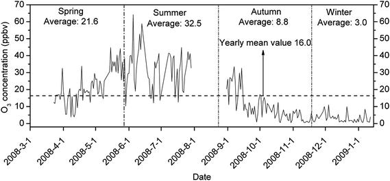

Fig. 2 Time series of daily average O₃ levels in Xi'an.

Monthly distributions generated from these daily averages are shown in Fig. 3 along with information for meteorological conditions (surface temperature, air pressure and relative humidity). The months of May to July had the highest O₃ levels while the winter months had the lowest O₃ levels. The monthly average O₃ in June (33.5 ppb) was nearly 12 times higher than in January (2.8 ppb). Note that no data was available in August. Earlier studies suggested that solar radiation was one of several important factors influencing O₃ production.³ Unfortunately, solar radiation data was not available to this study and temperature could be used as a surrogate measure of solar radiation to some extent. Apparently, temperature played a major role in the monthly variations of O₃ concentrations as can be seen from a comparison of Fig. 3a and 3b. However, it was noticed that the temperature in July was slightly higher than in June while O₃ levels in June were slightly higher than in July. This suggests that temperature is not a perfect surrogate for solar radiation as it can be very warm but cloudy. It may also suggest that other factors (e.g., emissions of O₃ precursors) are impact factors on O₃ levels.

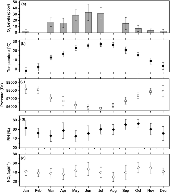Fig. 3 The monthly average of (a) O₃ concentrations, (b) ambient temperature, (c) ambient pressure, (d) relative humidity, and (e) NO₂ levels in Xi'an. Vertical bars indicate ±1 standard deviation of the daily average data. O₃ values for Feb and Aug 2008 are not available.

The statistical results of the daily average O₃ for each season, along with meteorological parameters, are listed in Table 1, while the frequency distributions of the hourly average O₃ concentration in four seasons are shown in Fig. 4. Note that the effective hourly data points from spring to winter were 1504, 1172, 2046 and 989, respectively. From the large monthly variations in O₃ levels discussed above, one can expect large seasonal differences as shown in Table 1 and Fig. 4. For example, in winter season, nearly 70% of the hourly data were under 2 ppbv and only ∼10% of the data were above 10 ppbv; in summer, only 19% of the hourly data were under 10 ppbv and 40% of the hourly data were higher than 30 ppb. O₃ levels in spring and autumn were much higher than in winter, but substantially smaller than in summer. The maximum hourly value reached 139.7 ppbv on 15 May 2008, which was on a different date for the maximum daily average value (June 5). Only 24 data points of hourly O₃ exceeded the China National Air Quality Standard value (102 ppbv); among these 8 points in spring, 15 in summer and 1 in autumn.

Table 1 Summary of seasonal variations of O₃ and meteorological factors

	Spring		Summer		Autumn		Winter		Annually
	Mean	S.D.	Mean	S.D.	Mean	S.D.	Mean	S.D.	Mean	S.D
O3 (ppbv)	21.8	10.1	32.5	11.6	8.8	8.1	3.0	2.5	16.0	13.8
WS (m s^−1)	1. 7	0. 6	1.7	0.4	1.4	0.5	2.9	0.5	1.5	0.5
T (°C)	19.3	4. 9	26.6	2.6	14.9	5.8	9.7	4.0	17.1	8.4
RH (%)	51.6	15.7	54.3	14.9	68.4	12.3	85.0	14.9	58.4	16.2
Pressure (kpa)	96.5	0.6	95.9	0.3	97.3	0.6	99.5	0.7	96.9	0.9

---

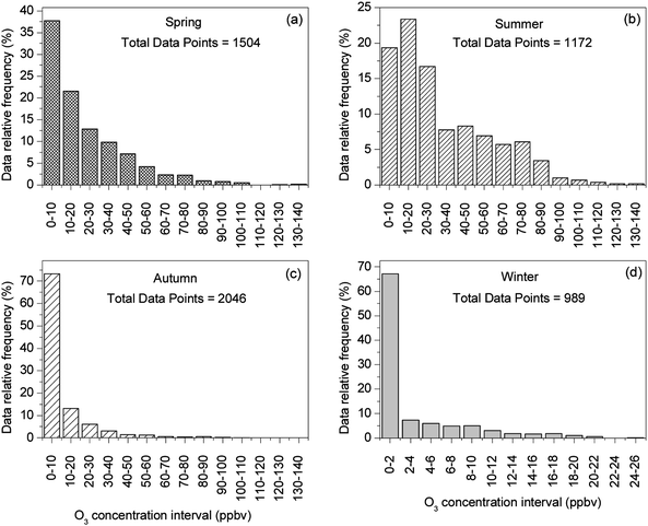Fig. 4 Frequency distribution of hourly O₃ data from March 2008 to January 2009.

The diurnal cycles of the hourly average O₃ concentrations are shown in Fig. 5. Theoretically, local O₃ production and depletion through NO_x and VOC chemistry, O₃mixing down from the free troposphere, surface O₃dry deposition, and to some extent, horizontal transportation, all played important roles in the observed diurnal patterns.^33–38 Data collected in this study showed that O₃ had a minimum in the early morning (6:00–8:00 local standard time (LST)), increased rapidly after sunrise, reached to the peak in the early afternoon (15:00–17:00 LST), decreased sharply in the late afternoon, continued decreasing slowly through the night, and decreased significantly in the early morning and reached the daily minimum. The maximum hourly average O₃ concentrations were 139.7 ppbv, 131.5 ppbv, 106.5 ppbv, and 22.6 ppbv from spring to winter, respectively, and the minimum values corresponded to 6.7 ppbv, 11.5 ppbv, 2.0 ppbv, and 0.1 ppbv, respectively. Apparently, the amplitudes of the O₃ diurnal cycle in warmer seasons were much larger than those in cold seasons.

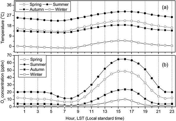Fig. 5 Diurnal cycle of (a) ambient temperature and (b) O₃ concentration.

NO emission from vehicles was not observed in this study, but is believed to have a typical diurnal pattern similar to other urban areas, that is with two peaks in a day related to the traffic rush hours in the morning (around 07:00 LST) and in the late afternoon (around 19:00 LST in weekdays).³⁵ Thus, the morning minimum between 6:00–8:00 should be caused by O₃ depletion by NO emissions from traffic, considering that the mixing layer was not yet fully developed and the O₃ photochemical production was still limited (due to the low UV as was seen from the low temperature in Fig. 5a). The subsequent increases and the peak in early afternoon (when the UV was strongest) in O₃ can be explained by the increased O₃ photochemical production and enhanced convection between free troposphere and boundary layer which brought ozone-rich air down to the surface. It should also be noted that NO emission during this period (mid morning to early afternoon) was also lower than traffic hours, so the O₃ photochemical production was more than the O₃ depletion. The same reasons caused the rapid decrease in O₃ in later afternoon. The continued, but much slower decrease through the night should be attributed to the surface deposition, depletion reaction, and possibly dilution and dispersion processes.^33–36 The stable boundary layer and the lack of solar radiation in the night prevented the replenishment of the depleted surface O₃.³⁷

The diurnal cycle of O₃ observed in Xi'an is typical and generally agreed with many other studies conducted elsewhere, e.g., Jinan, China,²¹ Guangzhou, China,²² Merced River, USA,⁷ Anantapur and Gadanki, India.^38,39 The diurnal variation of O₃ in rural or background sites also showed unimodal distribution (i.e. Lamas d'OLO a rural mountainous site in Portugal;⁴⁰ Shangdianzi background station in suburb of Beijing in China⁴¹). In contrast, a number of sites displayed bimodal distribution in their diurnal plots, with the first peak in the mid-morning and the other in the early evening (i.e. Mirror Lake in Yosemite National Park of USA;³⁷ the upper Rhine valley in TRACT area⁴²). Burley et al.³⁷ indicated that the formation of double-peaked maxima would be highly associated with the unique location and topography of sampling sites. Löffler-Mang et al.⁴² suggested that the first peak in the mid-morning was attributed to the morning break-up of the nocturnal stable boundary layer, with ozone-rich air mixing downwards from above. The second peak that arises a few hours later corresponds to the horizontal transport of air via up-valley winds.

3.2. Factors affecting O₃ formation over Xi'an

It is well known that three essential ingredients are needed for O₃ production in urban atmospheres: sunlight, NO_x, and hydrocarbons.⁴³ Temperature (as a surrogate of solar radiation) was thus well correlated with O₃ concentration as discussed above and shown in Fig. 3 and 5. The correlation coefficient (R) between temperature and O₃ concentration was as high as 0.8 (P < 0.001) from using all year data. The correlation was much higher if only using the daytime data. Since Xi'an is located at the semi-arid areas of northwest China, one would expect very low relative humidity (RH). However, the measured monthly average RH varied from 45.5% to 72.9%, with an annual average of 57.8%. This suggested that water vapor would not be a limiting factor in the O₃ production process. Note that water vapor is needed in the production of OH, which oxidizes hydrocarbons to produce peroxy radicals (RO₂), a middle product that reacts with NO_x to produce O₃. In fact, a negative correlation between RH and O₃ concentration was observed (R = −0.4, P < 0.001). This negative correlation was likely due to the fact that under low temperature conditions, RH was generally high (see Table 1) and O₃ were generally low. It is thus concluded that RH was not a limiting factor in O₃ production in this city and that RH did not control O₃ production significantly.

The net role of wind speed on surface O₃ should be location and time dependent. For example, high wind speed can increase the dilution of primary pollutants and thus decrease O₃ production.^44,45 This would suggest a high O₃ production under weak wind conditions; however, the reduction in dilution will be counterbalanced by the reduction in mixing from the upper layer.³⁵

The monthly averaged concentration of NO₂ ranged from 30.3 to 50.4 μg m⁻³ as shown in Fig. 3(e). The quite high concentrations of NO₂ and the relatively low concentrations of O₃ suggest that NO_x should not be a limiting factor in the production of O₃. This assumption was supported by the non-significant correlation between NO₂ and O₃. On the other hand, the concentrations of volatile organic carbon (VOC) might have played a limiting role in the ozone production as supported in discussions presented in Section 3.3 and 3.4 below.

3.3. O₃ episodes

The ozone episodes were defined here as hourly average concentrations exceeding the Chinese National Ambient Air Quality Standard Grade 2 (CNAAQS, 102 ppbv). There were a total of ten pollution episodes observed during the measurement period and they were all listed in Table 2. By comparison of meteorological conditions between ozone episodes (Table 2) and other periods (Table 1), it was found that high ozone days were mainly associated with low RH, high temperature, and zero rainfall. However, there seemed to be no association with low wind speeds, contrary to what was found in other studies.^19,22 For example, the hourly averaged wind speeds at 17:00 and 18:00 LST on 11 June exceeded 4.1 m s⁻¹. It was thus suspected that other factors might have also contributed to the high O₃ episodes. The air mass back-trajectory was used to identify the possible origin of O₃ or its precursors below.

Table 2 Ozone concentration and meteorological data during ozone pollution episodes

Date	Time (LST)	O3 (ppbv)	WS (m s^−1)	P (Pa)	T (°C)	RH (%)
2008-5-15	15:00	122.6	1.8	96 020	32.2	28
	16:00	139.7	1.9	95 930	33.3	25
	17:00	138.4	1.7	95 850	33.1	26
	18:00	105.1	1.6	95 830	32.5	27
2008-5-21	18:00	102.1	1.5	95 810	29.6	26
2008-5-23	15:00	103.6	2.7	95 880	31.6	25
2008-5-24	14:00	105.2	2.7	95 760	31.6	28
	15:00	107.7	2.2	95 680	32.2	29
2008-6-2	15:00	107.1	1.7	95 720	34.6	17
2008-6-5	14:00	116.4	2.3	95 520	32.6	25
	15:00	127.2	1.9	95 360	34.1	25
	16:00	130.1	3.1	95 240	34.3	23
	17:00	131.6	2.8	95 210	34.1	24
	18:00	126.0	2.6	95 180	33.8	25
	19:00	104.8	1.9	95 260	32.3	27
2008-6-11	14:00	106.5	2.2	96 060	31.6	32
	15:00	113.6	2.9	95 940	32.7	31
	16:00	119.2	3.5	95 850	32.4	32
	17:00	118.1	4.1	95 780	31.8	33
	18:00	103.1	4.1	95 790	30.5	36
2008-6-13	17:00	105.6	1.3	95 340	34.8	24
	18:00	103.4	1.8	95 320	34.5	24
2008-6-25	14:00	105.7	1.3	95 780	35.7	20
2008-9-4	18:00	106.5	1.5	96 090	30.6	31

---

Among the ten pollution episodes, three episodes, which happened on May 15, June 5 and 11, respectively, should be emphasized since these episodes lasted for more than 4 h (other episodes were all shorter than 3 h). On 15 May, the O₃ kept high levels during the daytime and sharply exceeded the standard level of 102 ppbv from 15:00 to 18:00 LST. The ozone concentration at 16:00 LST was the highest hourly level among the whole year of observations. Six and five hours, respectively, on June 5 and 11 exceeded the standard. These exceeding hours were all in the mid-afternoon, corresponding to the high temperature periods. 24 h air mass back-trajectories arriving at 100 m above ground level were calculated for the Xi'an station using the NOAA HYSPLIT 4 trajectory model to investigate the transport pathways and origin of surface O₃ or its precursors. As shown in Fig. 6, the air masses for 15 May mainly came from the region southwest of Xi'an. On June 5, air mass arriving at Xi'an passed through the southern area. While on June 11, the air mass mainly passed over the southern region, and then turned to the southeastern region, and then arrived at Xi'an.

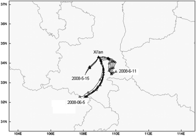Fig. 6 24 h air mass back-trajectory of ozone pollution episodes on May 15 (15:00–18:00 LST), June 5 (14:00–19:00 LST) and 11 (14:00–18:00 LST).

In general, the backward trajectories show that air masses arriving at Xi'an during the most severe three cases (15 May, 5 and 11 June) all came from southern regions of Xi'an, that's the Qinling Mountain areas, which is a lush growth of vegetation region in late spring, summer, and early autumn. Air masses passing through Qinling Mountain areas in the monsoon season were expected to have higher biogenic VOC. Biogenic VOC emissions could be a big part of the total VOC.⁴⁶ Previous modeling and measurement studies demonstrated that the oxygenated VOCs play important roles in determining the O₃ formation.^47,48 Curci et al.⁴⁹ demonstrated that emissions of oxygenated VOCs from vegetation, such as isoprene and terpene, increased on the summer daily ozone levels ranging from 1.5 to 15 ppbv in European regions. A study on PRD also showed that biogenic VOC was a major VOC emission source in the PRD region,⁵⁰ and biogenic VOCs have been shown to play important roles in regional ozone formation.⁵¹ Moreover, Studies on the relationship between O₃ and its precursors also revealed that O₃ production was VOC-limited in the urban areas, and possibly NO_x limited in the northern or northeastern rural areas of PRD.^22,52–57 Shao et al.⁵⁸ found that biogenic VOC, although contributed less than anthropogenic VOC to the total VOC, played a more important role in O₃ formation in the city of Guangzhou, China. Based on the back trajectories for the O₃ episode periods discussed above, it is very likely that the transportation of biogenic VOC from Qinling Mountain increased the total ambient VOC levels in Xi'an, and thus subsequently increased O₃ production during the O₃ pollution episodes.

It is also noted that, the 24 h air mass back-trajectories on 15 May were up to 3000 m, implying the possibility of vertical transport of ozone from upper levels down to the surface. Previous studies have shown that transport of ozone-rich air masses from the stratosphere to the troposphere is an important reason for the spring maximum.^19,59,60 For summer episodes, the backward trajectories all stayed below 1500 m, thus excluding the possibility of vertical transport. In these episodes, transportation of biogenic VOC seemed to have played an important role.

The wind-rose figure during O₃ episodes on May 15, June 5 and 11 was also plotted as shown in Fig. 7. Most of the surface wind directions were from the south of Xi'an city, which coincided with the air-mass trajectory results mentioned above. It further supported that biogenic VOC from the Qinling Mountain heavily influenced the urban O₃ production.

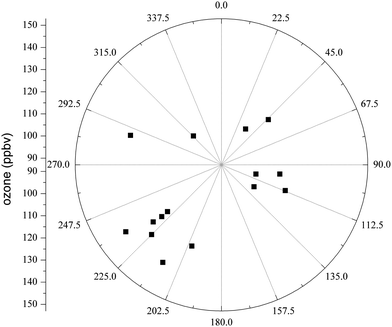Fig. 7 Wind-rose of the ozone pollution episodes on May 15 (15:00–18:00 LST), June 5 (14:00–19:00 LST) and 11 (14:00–18:00 LST).

3.4. Potential weekday and weekend differences

Weekday and weekend differences in ozone concentrations were typically found in metropolitan areas due to decreased traffic emissions on weekends.^61,62 The decrease of NO titration was an incontrovertible reason to enhance the O₃ levels at weekends. Wennberg and Dabdub⁴³ demonstrated that NO₂ concentration was another important factor for O₃ production, and it reported that when NO₂ levels become high, the loss of OH (hydroxyl free radicals) to nitric acid, HONO₂, slows the reactivity, and the rate of ozone production drops. For example, O₃ levels on weekends were much higher than on weekdays in Los Angeles, which reflected an evident O₃ weekend effect.⁶² To explore the potential weekday and weekend difference in Xi'an, Fig. 8 (a) displays the day of the week of O₃ concentration data. There were no significant differences between “weekend” and “weekday” in the mean (16.5 versus 16.2 ppbv), median (13.6 versus 11.8 ppbv) and the range of O₃ concentration data. One reason for this phenomenon could be due to the small differences in small NO₂ concentrations between “weekend” and “weekdays”. As shown in Fig. 8(b), the weekend NO₂ was only 5% smaller than weekday NO₂ in both mean (40.2 versus 42.4 μg m⁻³) and median values (39.0 versus 41.0 μg m⁻³). Zheng et al.²² also reported that there was no weekend effect about O₃ variation in Guangzhou, China, and it was mainly because of no statistically significant difference for NO₂ concentration between weekday and weekend. A recent investigation of traffic flows at the urban area of Guangzhou showed only a small (6.8%) decrease in the traffic flow between weekend and weekdays,⁵⁰ suggesting their comparable NO levels. It should be pointed out that at locations with low VOC emissions, O₃ production should be more sensitive to the change in VOC emissions than to the change in NO_x emissions. Further studies with more monitoring data including VOC concentration and theoretical studies using a mathematical model are needed to verify this assumption.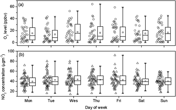

Fig. 8 Day of the week variations for O₃ (a) and NO₂ (b).

3.5 Comparison with other measurements

To get more insight into the characteristics of ground O₃ in Xi'an, data from the present study were compared with measurements from several other cities and rural areas in China and with some studies outside China (Table 3). The mean O₃ in Xi'an (16 ppb) was similar to one city in the PRD region (16.5 ppb),²² slightly lower than two cities in southern China, Shanghai (19 ppb)⁶³ and Nanjing (20.4 ppb),¹⁹ and much lower than one city in central China, Jinan (29.6 ppb).²¹ A combination of differences in NO_x and VOC emission and meteorological conditions caused these differences. It is also noted that O₃ levels in Xi'an and most other Chinese cities were much lower than O₃ levels in Chinese rural areas. Based on discussions in Section 3.3 and previous studies cited in the same section, it is believed the low biogenic VOC in cities was the main reason causing the city–rural differences. As mentioned earlier, although the concentration of biogenic VOC was not as high as anthropogenic VOC in some cities, its role on O₃ formation can be more important than anthropogenic VOC. The same theory might also explain the lower O₃ level in several Chinese cities compared to several cities outside China since the forest coverage in areas surrounding the Chinese cities mentioned above is relatively low.

Table 3 O₃ levels in different sites

Location	Site description	Observation period	Ozone levels mean (ppbv)	Reference
Xi'an, China	Uraban	March 2008–Feb. 2009	16.0	This study
Nanjing, China	Urban	Jan. 2000–Feb. 2003	20.4	Tu et al. (2007)^19
Shanghai, China	Urban	Jan.–Dec. 2002	19.0 ppb	zhang et al. (2003)^63
Jinan, China	Urban	June 2003–May 2004	29.6	Shan et al. (2008)^21
	Urban		16.5
PRD, China	Suburban	Jan. 2006–Dec. 2007	24.5	Zheng et al. (2010)^22
	Rural		36.0
	Coastal site		20.5
Beijing, China	Background	2004–2006	31.5 ppb	Lin et al. (2008)^41
Yangtze Delta Region, China	Background	1991–2006	17.5–52.3	Xu et al. (2008)^59
Waliguan, China	Rural	Aug.1994–Dec.2001	48.0 ppb	Nie et al. (2004)^64
Oki, Japan	Islands	Jan. 2001–Sept. 2002	23–60 ppb	Sikder et al. (2011)^65
Chicago, USA	Urban	1996–2000 (June–August)	39.2 ppb	Lin et al. (2010)^66
Anantapur, India	Urban	2001–2003	35.9	Ahammed et al. (2006)^67
Anantapur, India	Rural	Dec. 2008–July 2009	45.9	Reddy et al. (2010)^38
Tranquebar, India	Rural/coastal	May 1997–Oct. 2000	21.5	Debaje et al. (2003)^68
Kislovodsk, Russia	Background	1989–1998	46.6 ppb	Senik et al. (2001)^69
Southern France	Coastal area	Summers in 2001 and 2002	46.5 ppb	Dalstein et al. (2005)^70
	Rural		39.6 ppb (2002)

---

Prior study suggested that high aerosol loading in Chinese cities produced a lower UV flux, and then expected a lower O₃ concentration (Bian et al., 2007).⁷¹ While this assumption might be true, the impact of increased PM mass concentration might not be as large as the impact of biogenic VOC emission in the formation of O₃ in Xi'an.

4. Conclusions

Surface ozone was monitored in a northwestern city of China, Xi'an, for a one year period. Seasonal and diurnal patterns generally agreed with measurements made in other cities and can be mostly explained by meteorological factors. The highest O₃ levels appeared in the early afternoon and in hot seasons while the lowest O₃ levels appeared in early morning and in cold seasons. The longest O₃ episodes were found to be linked with air masses containing high biogenic VOC emissions which originated from vegetation of the Qinling Mountains. Mean O₃ levels in Xi'an were of a similar order of magnitude to several other Chinese cities in southern China, although lower than many cities outside China. Future measurement studies on O₃ should also include concurrent measurements of NO_x and VOC and key meteorological parameters in order to better understand O₃ formation mechanism and limiting factors. Mathematical models can also be used in combination of measurement data to improve our knowledge on this topic and to provide theoretical basis for making emission policy decisions.

Acknowledgements

This research is supported by the Fundamental Research Funds for the Central University of China (XJJ20100130), the Chinese Academy of Sciences (O929011018), and the SKLLQG, Chinese Academy of Sciences (grant SKLLQG1010).

References

1. IPCC: Climate change 2007 – Synthesis Report, 2007.
2. P. Solomon, E. Cowling and G. Hidy, et al., Comparison of scientific findings from major ozone field studies in North America and Europe, Atmos. Environ., 2000, 34, 1885–920.
3. M. L. Thompson, J. Reynolds and L. H. Cox, et al., A review of statistical methods for the meteorological adjustment of tropospheric ozone, Atmos. Environ., 2001, 35, 617–30.
4. R. Vingarzan, A review of surface ozone background levels and trends, Atmos. Environ., 2004, 38, 3431–42.
5. B. J. Mulholland, J. Craigon and C. R. Black, et al., Effects of elevated CO₂ and O₃ on the rate and duration of grain growth and harvest index in spring wheat (Triticum aestivum L.), Global Change Biol., 1998, 4, 627–35.
6. P. H. Fischer, B. Brunekreef and E. Lebret, Air pollution related deaths during the 2003 heat wave in the Netherlands, Atmos. Environ., 2004, 38, 1083–5.
7. X. Wang, W. Lu and W. Wang, et al., A study of ozone variation trend within area of affecting human health in Hong Kong, Chemosphere, 2003, 52, 1405–10.
8. F. De Leeuw, Trends in ground level ozone concentrations in the European Union, Environ. Sci. Policy, 2000, 3, 189–99.
9. M. Coyle, D. Fowler and M. Ashmore, New directions, implications of increasing tropospheric background ozone concentrations for vegetation, Atmos. Environ., 2003, 37(1), 153–4.
10. S. BrÖnnimann, B. Buchmann and H. Wanner, Trends in near-surface ozone concentrations in Switzerland: the 1990s, Atmos. Environ., 2002, 36, 2841–2852.
11. S. B. Jonnalagadda, J. Bwila and W. Kosmus, Surface ozone concentrations in Eastern Highlands of Zimbabwe, Atmos. Environ., 2001, 35, 4341–6.
12. M. A. García, M. L. Sánchez and I. A. Pérez, et al., Ground level ozone concentrations at a rural location in northern Spain, Sci, Sci. Total Environ., 2005, 348, 135–50.
13. P. Sicard, L. Dalstein-Richier and N. Vas, Annual and seasonal trends of ambient ozone concentration and its impact on forest vegetation in Mercantour National Park (South-eastern France) over the 2000–2008 period, Environ. Pollut., 2011, 159, 351–62.
14. D. R. Hastie, J. Narayan and C. Sciller, et al., Observational evidence for the impact of the lake breeze circulation on ozone concentrations in Southern Ontario, Atmos. Environ., 1999, 33, 323–35.
15. E. Brankov, R. Henry and K. Civerolo, et al., Assessing the effects of transboundary ozone pollution between Ontario, Canada and New York, USA, Environ. Pollut., 2003, 123, 403–11.
16. H. X. Wang, C. S. Kiang and X. Y. Tang, et al., Surface ozone: a likely threat to crops in Yangtze delta of China, Atmos. Environ., 2005, 39, 3843–50.
17. X. K. Wang, W. Manning and Z. W. Feng, et al., Ground-level ozone in China: distribution and effects on crop yields, Environ. Pollut., 2007, 147, 394–400.
18. D. G. Streets, J. S. Fu and C. J. Jang, et al., Air quality during the 2008 Beijing Olympic Games, Atmos. Environ., 2007, 41, 480–92.
19. J. Tu, Z. G. Xia and H. S. Wang, et al., Temporal variations in surface ozone and its precursors and meteorological effects at an urban site in China, Atmos. Res., 2007, 85, 310–37.
20. K. S. Lam, T. J. Wang and C. L. Wu, et al., Study on an ozone episode in hot season in Hong Kong and transboundary air pollution over Pearl River Delta region of China, Atmos. Environ., 2005, 39, 1967–77.
21. W. Shan, Y. Yin and J. Zhang, et al., Observational study of surface ozone at an urban site in East China, Atmos. Res., 2008, 89, 252–61.
22. J. Zheng, L. Zhong and T. Wang, et al., Ground-level ozone in the Pearl River Delta region: Analysis of data from a recently established regional air quality monitoring network, Atmos. Environ., 2010, 44, 814–23.
23. W. Shan, J. Zhang and Z. Huang, et al., Characterizations of ozone and related compounds under the influence of maritime and continental winds at a coastal site in the Yangtze Delta, nearby Shanghai, Atmos. Res., 2010, 97, 26–34.
24. H. W. Y. Wu and L. Y. Chan, Surface ozone trends in Hong Kong in 1985–1995, Environ. Int., 2001, 26, 213–22.
25. J. J. Cao, F. Wu and J. C. Chow, et al., Characterization and source apportionment of atmospheric organic and elemental carbon during fall and winter of 2003 in Xi'an, China, Atmos. Chem. Phys., 2005, 5, 3127–37.
26. J. J. Cao, S. C. Lee and X. Y. Zhang, et al., Characterization of airborne carbonate over a site near Asian dust source regions during spring 2002 and its climatic and environmental significance, J. Geophys. Res., 2005, 110, D03203,  DOI:10.1029/2004JD005244.
27. J. J. Cao, C. S. Zhu and J. C. Chow, et al., Black carbon relationships with emissions and meteorology in Xi'an, China, Atmos. Res., 2009, 94, 194–202.
28. Z. X. Shen, R. Arimoto and J. J. Cao, et al., Seasonal variations and evidence for the effectiveness of pollution controls on water-soluble inorganic species in total suspended particulates and fine particulate matter from Xi'an, China, J. Air Waste Manage. Assoc., 2008, 58, 1560–70.
29. Z. X. Shen, J. J. Cao and R. Arimoto, et al., Ionic composition of TSP and PM_2.5 during dust storms and air pollution episodes at Xi'an, China, Atmos. Environ., 2009, 43, 2911–8.
30. Z. X. Shen, J. J. Cao and R. Arimoto, et al., Chemical characteristics of fine particles (PM₁) over Xi'an, China, Aerosol Sci. Technol., 2010, 44, 461–72.
31. UNEP, Independent Environmental Assessment-Beijing 2008 Olympic Games, 2009, pp. 27.
32. Who, WHO air quality guidelines for particulate matter, ozone, nitrogen dioxide and sulphur dioxide, Summary of risk assessment, 2005, pp. 9.
33. W. L. Chameides and J. G. Walker, A time-dependent photochemical model for ozone near the ground, J. Geophys. Res., 1976, 81, 413–423.
34. J. A. Garland and R. G. Derwent, Destruction at the ground and the diurnal cycle of concentration of ozone and other gases, Q. J. R. Meteorol. Soc., 1979, 105, 169–183.
35. Porg, Ozone in the United Kingdom, Fourth Report of the Photochemical Oxidants Review Group, The Department of the Environment Transport and the Regions, Edinburgh, 1988.
36. M. Coyle, R. I. Smith and J. R. Stedman, et al., Quantifying the spatial distribution of surface ozone concentration in the UK, Atmos. Environ., 2002, 36, 1013–1024.
37. J. D. Burley and J. D. Ray, Surface ozone in Yosemite National Park, Atmos. Environ., 2007, 41, 6048–62.
38. B. S. K. Reddy, K. R. Kumar and G. Balakrishnaiah, et al., Observational studies on the variations in surface ozone concentration at Anantapur in southern India, Atmos. Res., 2010, 98, 125–39.
39. N. Naja, H. Akimoto and J. Staehelin, Ozone in background and photochemically aged air over central Europe: analysis of long-term ozonesonde data from hohenpeissenberg and payerne, J. Geophys. Res., 2003, 108, 4063,  DOI:10.1029/2002JD002477.
40. A. Carvalho, A. Monteiro and I. Ribeiro, et al., High ozone levels in the northeast of Portugal: Analysis and characterization, Atmos. Environ., 2010, 44, 1020–31.
41. W. Lin, X. Xu and X. Zhang, et al., Contributions of pollutants from North China Plain to surface ozone at the Shangdianzi GAW station, Atmos. Chem. Phys. Discuss., 2008, 8, 9139–65.
42. M. Löffler-Mang and J. Joss, An Optical Disdrometer for Measuring Size and Velocity of Hydrometeors, J. Atmos. Oceanic Technol., 2000, 17, 130–9.
43. P. O. Wennberg and D. Dabdub, Rethinking Ozone Production, Science, 2008, 319, 1624–5.
44. D. Xu, D. Yap and P. A. Taylor, Meteorologically adjusted ground level ozone trends in Ontario, Atmos. Environ., 1996, 30, 1117–24.
45. C. Dueñas, M. C. Fernández and S. Cañete, et al., Assessment of ozone variations and meteorological effects in an urban area in the Mediterranean Coast, Sci. Total Environ., 2002, 299, 97–113.
46. E. Diem Jeremy, Comparisons of weekday-weekend ozone: importance of biogenic volatile organic compound emissions in the semi-arid southwest USA, Atmos. Environ., 2000, 34, 3445–51.
47. F. H. Geng, X. X. Tie and J. M. Xu, et al., Characterizations of ozone, NO_x, and VOCs measured in Shanghai, China, Atmos. Environ., 2008, 42, 6873–83.
48. X. Tie, S. Madronich and G. Li, et al., Simulation of Mexico City plumes during the MIRAGE-Mex field campaign using the WRF-Chem model, Atmos. Chem. Phys., 2009, 9, 4621–38.
49. G. Curci, M. Beekmann and R. Vautard, et al., Modelling study of the impact of isoprene and terpene biogenic emissions on European ozone levels, Atmos. Environ., 2009, 43, 1444–55.
50. J. Y. Zheng, L. J. Zhang and W. W. Che, et al., A highly resolved temporal and spatial air pollutant emission inventory for the Pearl River Delta region, China and its uncertainty assessment, Atmos. Environ., 2009, 43, 5112–22.
51. X. L. Wei, Y. S. Li and K. S. Lam, et al., Impact of biogenic VOC emissions on a tropical cyclone-related ozone episode in the Pearl River Delta region, China, Atmos. Environ., 2007, 41, 7851–64.
52. K. L. So and T. Wang, C₃–C₁₂ non-methane hydrocarbons in subtropical Hong Kong: spatial-temporal variations, source-receptor relationships and photochemical reactivity, Sci, Sci. Total Environ., 2004, 328, 161–74.
53. J. P. Huang, J. C. H. Fung and A. K. H. Lau, et al., Numerical simulation and process analysis of typhoon-related ozone episodes in Hong Kong, J. Geophys. Res., 2005, 110, D05301,  DOI:10.1029/2004JD004914.
54. J. Zhang, T. Wang and W. L. Chameides, et al., Ozone production and hydrocarbon reactivity in Hong Kong, Southern China, Atmos. Chem. Phys., 2007, 7, 557–73.
55. Y. H. Zhang, H. Su and L. J. Zhong, et al., Regional ozone pollution and observation-based approach for analyzing ozone-precursor relationship during the PRIDE-PRD2004 campaign, Atmos. Environ., 2008, 42, 6203–18.
56. H. R. Cheng, H. Guo and X. M. Wang, et al., On the relationship between ozone and its precursors in the Pearl River Delta: application of an observation-based model (OBM), Environ. Sci. Pollut. Res., 2010a, 17, 547–60.
57. H. R. Cheng, H. Guo and S. M. Saunders, et al., Assessing photochemical ozone formation in the Pearl River Delta with a photochemical trajectory model, Atmos. Environ., 2010, 44, 4199–208.
58. M. Shao, M. Zhao and Y. Zhang, et al., Biogenic VOCs emissions and its impact on ozone formation in major cities of China, J. Environ. Sci. Health., A, 2000, 35, 1941–50.
59. X. Xu, W. Lin and T. Wang, et al., Long-term trend of surface ozone at a regional background station in eastern China 1991–2006: enhanced variability, Atmos. Chem. Phys., 2008, 8, 2595–607.
60. K. Yamaji, J. Li and I. Uno, et al., Impact of open crop residual burning on air quality over Central Eastern China during the Mount Tai Experiment 2006 (MTX2006), Atmos. Chem. Phys., 2010, 10, 7353–68.
61. V. Pont and J. Fontan, Comparison between weekend and weekday ozone concentration in large cities in France, Atmos. Environ., 2001, 35, 1527–35.
62. G. Yarwood, T. E. Stoeckenius and J. G. Heiken, et al., Modeling weekday/weekend ozone differences in the Los Angeles region for 1997, J. Air. Waste Manage., 2003, 53, 864–75.
63. Y. Zhang, Y. Zheng and W. Lou, State of ozone pollution and its change in the center urban area of Shanghai, Environmental Monitoring Management and Technology, 2003, 15, 15–20 (in Chinese).
64. H. Nie, S. Nie and Z. Wang, et al., Characteristic analysis of surface ozone over clean area in Qinghai-Tibet Plateau, Arid. Meteorology., 2004, 22, 1–7 (in Chinese).
65. H. A. Sikder, J. Suthawaree and S. Kato, et al., Surface ozone and carbon monoxide levels observed at Oki, Japan: Regional air pollution trends in East Asia, J. Environ. Manage., 2011, 92, 953–9.
66. J. T. Lin, D. J. Wuebbles and H. C. Huang, et al., Potential effects of climate and emissions changes on surface ozone in the Chicago area, J. Great Lakes Res., 2010, 36, 59–64.
67. Y. N. Ahammed, R. R. Reddy and K. R. Gopal, et al., Seasonal variation of the surface ozone and its precursor gases during 2001–2003, measured at Anantapur (14.62°N), a semi-arid site in India, Atmos. Res., 2006, 80(2–3), 151–64.
68. S. B. Debaje, S. J. Jeyakumar and K. Ganesan, et al., Surface ozone measurements at tropical rural coastal station Tranquebar, India, A, Atmos. Environ., 2003, 37, 4911–6.
69. I. A. Senik and N. F. Elansky, Surface Ozone Concentration Measurements at the Kislovodsk High-Altitude Scientific Station: Temporal Variations and Trends, Izy. Atmos. Ocean. Phy., 2001, 37, 110–9.
70. L. Dalstein and N. Vas, Ozone Concentrations and Ozone-Induced Symptoms On Coastal and Alpine Mediterranean Pines in Southern France, Water, Air, Soil Pollut., 2005, 160, 181–95.
71. H. Bian, S. Q. Han and X. X. Tie, et al., Evidence of impact of aerosols on surface ozone concentration in Tianjin, China, Atmos. Environ., 2007, 41, 4672–81.

---