Determination of diesel cetane number by consensus modeling based on uninformative variable elimination

Abstract

Consensus modeling based on improved Boosting algorithm (Boosting-PLS, BPLS) combined with wavelength (variable) selection by MC-UVE (Monte Carlo-Uninformative Variable Elimination) method is applied to determination of cetane number (CN) of diesel. MC-UVE is firstly used to select characteristic variables from Near-infrared (NIR) spectra of diesel based on principles of MC simulation and UVE, and then the selected variables instead of the full spectra are used for BPLS modeling to predict results. From predicted results, the proposed MC-UVE-BPLS algorithm improves the performance of conventional linear PLS modeling in terms of accuracy and robustness, so it is more efficient and parsimonious with few numbers of useful variables when applied to the relationship between CN and diesel NIR spectra. Simultaneously, the prediction results of MC-UVE-BPLS compared with those of MC-UVE-PLS, BPLS and CPLS (Consensus modeling based on Bagging) show that MC-UVE-BPLS is superior to other models, and also verifies the efficiency of MC-UVE and improved BPLS. So the proposed MC-UVE-BPLS method provides a new approach for determination of diesel CN by NIR spectra.

---

1 Introduction

Near-infrared (NIR) spectra mainly come from the structure of the groups of a variety of X–H, which are contained in all kinds of compounds in petroleum products. Therefore, NIRs are used in all aspects of petrochemical detection^1,2 and play an important role with its technical characteristics of simple, rapid, nondestructive, reproducible, etc. Diesel spectra are very complex, and spectral overlaps are serious as a result of complex mixture of hydrocarbons. Therefore, diesel NIR data pre-processing³ to establish the model between its properties (e.g., cetane number, density, freezing point, distillation temperature, etc.) and the spectral data, is the key step for ensuring the accuracy of oil quality indicators.

Diesel cetane number (CN) is a key indicator for measuring diesel combustion. ASTMD 613 test method is an internationally traditional determination method of CN. GB/T 386 test method developed in China also references to ASTMD 613 method, which requires a lot of oil samples, is time-consuming and expensive. At present, NIR spectra for the determination of CN in diesel fuel have been reported.^4–7 Generally agreed that for non-linear relationship between diesel CN and spectral signals, non-linear support vector machine algorithm, artificial neural network, etc. is superior to linear modeling such as multiple linear regression and partial least squares (PLS) algorithms, etc. And it is found that few variable selection method^4,7 is used for pre-processing of diesel spectrum signal.

In this article, Monte Carlo-Uninformative Variable Elimination (MC-UVE) method was first adopted to select characteristic wavelengths (variables) from diesel original NIR signals. Sample-specific or component-specific information remained, and useless information was abandoned. As a result, the calibration modeling was proven and predigested significantly with fewer variables. MC-UVE method was combined with improved consensus PLS method based on Boosting (called BPLS) to build MC-UVE-BPLS modeling, which enhanced PLS linear modeling ability in predicting diesel CN in terms of accuracy and robustness for non-linear relationship between diesel CN and spectral signal. Compared with the full-spectrum method of BPLS, consensus PLS method based on Bagging (called CPLS) and conventional PLS method, it was found that MC-UVE-BPLS modeling obtained better prediction efficiency. Simultaneously, better predicted results were also obtained when compared with MC-UVE-PLS method without consensus strategy.

2 Theory and algorithm

2.1 MC-UVE-PLS

Uninformative variable elimination by PLS (UVE-PLS)^8,9 is a method of selecting wavelengths based on an analysis of regression coefficients of PLS, and it is the most popular variables selection method widely applied in analytical chemistry. MC simulation technique is effective to deal with complex multi-variable problems. Monte Carlo cross-validation (MCCV)¹⁰ is a very effective method decreasing the danger of overfit and underfit, to evaluate model capability including linear and non-linear modeling evaluation, factor number selection and modeling robustness, etc. in multiple regression analysis.

In this work, MC cross-validation was introduced in UVE-PLS to establish MC-UVE-PLS method, which had been applied in NIR data pre-processing, and got more accurate and robust prediction results than UVE-PLS method.¹¹

2.2 BPLS method

The basic idea of consensus strategy is predicting samples by utilizing multiple individual calibration models (called member models) constructed by different training subsets chosen from the same training set, which usually can obtain more accurate and robust prediction results than single model. Among common consensus modeling, CPLS algorithm based on Bagging (Bootstrap aggregating) sampling technique^12,13 randomly extracts training subsets of constant number from the whole training set, and takes the simple average of prediction results of all member models as the final prediction results.

Consensus algorithm based on Boosting sampling technique is adopted in this essay,¹⁴ which is modified on the basis of AdaBoost algorithm (one case of Boosting algorithm).¹⁵ The relative prediction errors between prediction value and true value (experimental value) of every sample in the training set are immediately used to update the resampling weights of samples. This is instead of using the absolute prediction errors between them, which are due to values of absolute prediction error of different samples or especially different property samples which sometimes differ greatly, so frequently modeling prediction ability can not be well reflected. Furthermore, relative to adding “robust” processes to BPLS in other research,¹⁶ the BPLS process proposed in this study is simple and intuitive, and retains the AdaBoost algorithm virtue of adjusting the number of iterations, and not needing to adjust any other parameters.

BPLS based on modified Boosting combined with PLS regression algorithm firstly constructs multiple models, which are trained individually, and then their predictions are combined by weighted averaging. The brief flowchart of the algorithm is given in Fig. 1 and the corresponding detailed procedures can be described as follows:

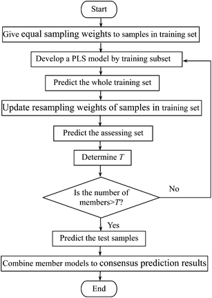Fig. 1 Flowchart of the BPLS algorithm.

(1) All the samples in the calibration set start with equal sampling weights 1/n (n is the number of samples in the calibration set). Individual PLS model C_t is established by picking up 63%¹⁷ of the samples from the whole calibration set according to the sample sampling weights.

(2) Predict samples of the whole calibration set with model C_t, and then calculate the relative prediction errors (δ_i,t) between prediction value and true value of every sample x_i in calibration set.

where y_i is the true corresponding value to x_i,t is the current iteration number (t = 1,…,T), e_i,t is the absolute prediction errors between prediction value and true value of sample x_i. Then δ_i,t are normalized and calculated by weighted mean to get prediction error δ_t of model C_twhere D_i (x_i) is the sampling weight of sample x_i. Then weight α_t of model C_t is

Finally, update the resampling weights of samples in calibration set according to formula (4), and then new weights are normalized.

(3) During every iteration process, step (2) is repeated, and results of prediction set are predicted by model C_t. The iteration is finished when the prediction error of samples in assessing the set starts to be stabilized. The ensemble prediction results are obtained by the weighted mean of the member models C_t in the boosting series using the following formula.

2.3 MC-UVE-BPLS

MC-UVE-BPLS method is the combination of MC-UVE and BPLS, in which MC-UVE first used to select characteristic wavelengths (variables) to replace raw NIR spectra of diesel. Hereafter, modeling by BPLS method is used to predict CN of diesel.

3 Experimental and calculations

Experimental datasets are provided by http://software.eigenvector.com/Data/SWRI/index.html. NIR spectra of 245 diesel samples were recorded in the wavelength range 750–1550 nm with the digitization interval ca. 2 nm, and each spectrum is composed of 401 data points. An example of the measured NIR spectra of diesel is given in Fig. 2.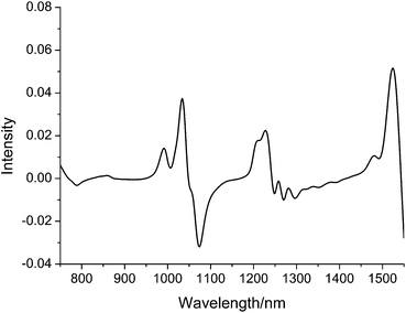

Fig. 2 An example of the measured NIR spectra of diesel.

245 samples (or spectra) were arbitrarily divided into three sets. 155 samples were used for calibration data set, 45 samples were used for assessing data set, and the remaining 45 samples were used for prediction data set.

In the comparison of MC-UVE-PLS, BPLS, CPLS and PLS methods, the same calibration set and prediction set were adopted. In the optimization of the parameters, the root mean squared error of prediction (RMSEP) was used as an evaluation criterion. RMSEP is defined as

where ŷ_i is the prediction concentration of the ith sample, y_i is the true concentration of the ith sample, and n is the number of prediction samples.

Matlab 6.5 is used as the model calculation software.

4 Results and discussions

4.1 Determination of number of principal factor

The number of principal factor (n_f) is an important parameter in PLS modeling. Too little principal factor will cause the model underfitting, and on the contrary, too much principal factor number will lead to the model overfitting, thus reduce the model prediction precision. In this study, principal factor numbers 1∼20 are investigated. Fig. 3 shows the variation of RMSEP for assessing data set with varying principal factor number.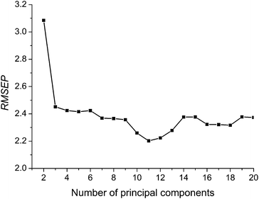

Fig. 3 Variation of RMSEPversus the number of principal components.

In Fig. 3, it can be seen that model accuracy changes with different principal factor number of PLS. At first, values of RMSEP are large and unstable. RMSEP descends gradually with the increase of principal factor number, but RMSEP have an increasing trend after n_f > 11. Therefore, n_f = 11 is used for further calculations in all five methods of MC-UVE-BPLS, MC-UVE-PLS, BPLS, CPLS and PLS.

4.2 Variables selection

Fig. 4 shows the stability of each variable in the wavelength 750–1550 nm by UVE method. In the figure, the dot lines show the cutoff values, which is determined by N_j = 130. Variables whose stability lies within the dot lines will be cut off, and the variables whose stability lies out of the dot lines are used for modeling.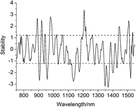

Fig. 4 The stability distribution of each variable by MC-UVE method.

It can be seen from Fig. 4, that the distributions of the stability are relatively dispersed, which is maybe caused by a total amount of multiple components in diesel including aromatics, naphthenes, alkanes, alkenes, etc., that is, absorptions of diesel NIR spectra contain a variety of groups of methyl, methylene, vinyl and aryl, etc.

In Fig. 4, the selected variables are concentrated on wavelength 818–988 nm, and several wavelengths around 1134, 1174, 1206 nm. In addition, some narrow wavelength intervals retained in the range of 1342–1534 nm. It is estimated that these bands are respectively assigned to frequency absorptions of C–H groups involved in functional groups of methyl, methylene, vinyl and aryl; double frequency absorptions of partial C–H groups involved in methyl and methylene; double frequency absorptions of C–H groups existed in all kinds of groups.¹⁸

A suitable number of reserved variables (N_j) is an important parameter to affect the stability and accuracy of the model. When the number of reserved variables is below N_j, the robustness and accuracy of the model will be poor, due to informative variables not completely remained. On the contrary, if the number of reserved variables is larger than N_j, uninformative variables should be embodied, resulting in bad performance of the model. N_j is investigated with steps of 20 from 30 to 300. For each N_j, a PLS model is developed and then the model is used to predict the assessing set. The mean value of RMSEP and the standard error of RMSEP (σ) of the assessing results through 50 repeated runs are shown in Fig. 5.

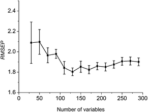Fig. 5 Variation of RMSEPs with the number of selected wavelengths. Standard deviation of 50 runs results is plotted as an error bar crossing the mean value.

Clearly, Fig. 5 shows that, at the beginning, the mean value and the standard error are both large, then both reduce gradually with the increase of N_j. When N_j is 130, the mean value is the lowest, and the standard error is also small. When N_j is bigger than 130, the mean value increases slightly with the increase of N_j. Accordingly, N_j = 130 is used for further study.

4.3 Determination of iteration number of BPLS

In Boosting-PLS modeling, iteration number (or member model number) is a vital parameter, which enormously influences prediction ability and prediction results of the model. In other research on Boosting, criterions of iteration termination are decided by directly setting a maximum number of iterations or a predetermined threshold of fitting error,¹⁹ which needs the experience of judgment, and can not guarantee model performance in prediction of different data. RMSEP of assessing set is directly chosen as the criterion of iteration number in this study, and relationships between iteration number and RMSEP of assessing set are studied.

Fig. 6 shows variations between RMSEP of assessing set and iteration time during 1800 iterations. RMSEP is high and instable when iteration number is small. RMSEP decreases with the increase of iteration time, and the variations of RMSEP tend to be slowed down. When iteration number is 1300, RMSEP reaches a minimum. Then RMSEP rises when iteration number exceeds 1300. The above situation coincides with the theory of consensus strategy, that is, an ideal combined system should consist of several accurate models that disagree in prediction as much as possible.²⁰ Finally, iteration number of 1300 is used for further study.

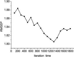Fig. 6 Variation between prediction error and iteration time.

4.4 Comparisons of MC-UVE-BPLS, MC-UVE-PLS, BPLS, CPLS and PLS

With the optimal parameters discussed above, MC-UVE-BPLS model is developed to predict CN of the 45 samples in the predicting set. The process is repeated 30 times, and the prediction results are compared with those of MC-UVE-PLS, BPLS, CPLS and PLS model (with the same data sets and parameters as in MC-UVE-BPLS). The mean RMSEP with their standard deviation (σ) were summarized in Table 1. The recovery ranges of 30 runs are also listed in Table 1.

Table 1 A comparison of the results obtained by different methods

Method	RMSEP (σ)	Recovery
MC-UVE-BPLS	2.089(0.007)	87.96–110.09
MC-UVE-PLS	2.142(0.010)	87.27–113.39
BPLS	2.143(0.005)	87.63–110.20
CPLS	2.255(0.002)	87.74–111.56
PLS	2.308(0.067)	86.24–117.32

---

It is found from Table 1, that the proposed MC-UVE-BPLS model improves the performance of conventional linear PLS modeling with few variables in predicting diesel CN from terms of accuracy and robustness. The results of MC-UVE-BPLS compared with BPLS and CPLS modeling with full-spectrum indicate that, wavelength selection by MC-UVE method is able to promote modeling ability and predigest modeling. The results of MC-UVE-BPLS are superior to MC-UVE-PLS, which reflects advantages of consensus modeling based on Boosting. Taken overall, the performance of MC-UVE-BPLS is superior to other models studied in dealing with NIR spectra signals.

It is also concluded that from Table 1, equivalent prediction results are obtained by MC-UVE-PLS with fewer wavelengths compared with the prediction results of BPLS. Simultaneously, for the data in this study, BPLS method based on Boosting obtains more accurate results than CPLS method based on Bagging.

5 Conclusions

MC-UVE-BPLS modeling is proposed to determine CN of diesel by NIR spectra. In the modeling, the spectra are firstly pretreated by MC-UVE method, and then predict samples by consensus model of BPLS. The prediction results of MC-UVE-BPLS are better than conventional PLS linear model, MC-UVE-PLS, BPLS and CPLS modeling in terms of accuracy or robustness. MC-UVE-BPLS modeling has advantages of efficiency and is inexpensive, so is a new method for quantitative analysis of NIR spectra and measurement of CN of diesel fuels.

Acknowledgements

This study is supported by the Natural Science Foundation of Hebei Province, China (No. B2011502061) and the Fundamental Research Funds for the Central Universities (No. 09QL52).

References

1. S. Macho and M. S. Larrechi, Anal. Chem., 2002, 21(12), 799–806.
2. J. J. Kelly, C. H. Barlow, T. M. Jinguji and J. B. Callis, Anal. Chem., 1989, 61, 313–320.
3. X. L. Chu, H. F. Yuan and W. Z. Lu, Prog. Chem. (in Chinese), 2004, 16(4), 528–542.
4. Z. Boger, Anal. Chim. Acta, 2003, 490, 31–40.
5. L. M. Fang and M. Lin, Acta Petrolei Sinica (Petroleum Processing Section)(in Chinese), 2008, 24(6), 726–732.
6. F. B. Gonzaga and C. Pasquini, Anal. Chim. Acta, 2010, 670, 92–97.
7. F. Rossi, D. Francois, V. Wertz, M. Meurens and M. Verleysen, Chemom. Intell. Lab. Syst., 2007, 86, 208–218.
8. V. Centner, D. L. Massart and O. E. de Noord, Anal. Chem., 1996, 68, 3851–3858.
9. C. Tan, J. Y. Wang, T. Wu, X. Qin and M. L. Li, Spectrochim. Acta, Part A, 2010, 77, 960–964.
10. Y. P. Du, S. Kasemsumran, K. Maruo, T. Nakagawa and Y. Ozaki, Chemom. Intell. Lab. Syst., 2006, 82, 83–89.
11. W. S. Cai, Y. K. Li and X. G. Shao, Chemom. Intell. Lab. Syst., 2008, 90(2), 188–194.
12. Y. K. Li, X. G. Shao and W. S. Cai, Chem. J Chinese U (in Chinese), 2007, 28(2), 246–249.
13. Y. K. Li, X. G. Shao and W. S. Cai, Talanta, 2007, 72(1), 217–222.
14. X. G. Shao, X. H. Bian and W. S. Cai, Anal. Chim. Acta, 2010, 666(1–2), 32–37.
15. R. Meir and G. Ratsch, In Advanced Lectures on Machine Learning, LNCS, 2003, pp. 119–184.
16. Y. P. Zhou, C. B. Cai, S. Huan, J. H. Jiang, H. L. Wu, G. L. Shen and R. Q. Yu, Anal. Chim. Acta, 2007, 593, 68–74.
17. L. Breiman, Mach. Learn., 1996, 24, 123–140.
18. A. A. christy, S. Kasemsumran, Y. P. Du and Y. Ozaki, Anal. Sci., 2004, 4(20), 935–940.
19. N. Duffy and D. Helmbold, Mach. Learn., 2002, 47, 153–200.
20. A. Krogh and J. Vedelsby, In Advances in Neural Information Processing Systems, MIT Press, Cambridge, MA, 1995, 7, pp. 231–238.

---