Electrostatics at the nanoscale
David A.
Walker
a,
Bartlomiej
Kowalczyk
ab,
Monica Olvera
de la Cruz
abc and
Bartosz A.
Grzybowski
*ab
aDepartment of Chemical and Biological Engineering, Northwestern University, 2145 Sheridan Road, Evanston, Illinois 60208, USA. E-mail: grzybor@norhwestern.edu
bDepartment of Chemistry, Northwestern University, 2145 Sheridan Road, Evanston, Illinois 60208, USA
cDepartment of Materials Science and Engineering, Northwestern University, 2145 Sheridan Road, Evanston, Illinois 60208, USA
First published on 14th February 2011
Abstract
Electrostatic forces are amongst the most versatile interactions to mediate the assembly of nanostructured materials. Depending on experimental conditions, these forces can be long- or short-ranged, can be either attractive or repulsive, and their directionality can be controlled by the shapes of the charged nano-objects. This Review is intended to serve as a primer for experimentalists curious about the fundamentals of nanoscale electrostatics and for theorists wishing to learn about recent experimental advances in the field. Accordingly, the first portion introduces the theoretical models of electrostatic double layers and derives electrostatic interaction potentials applicable to particles of different sizes and/or shapes and under different experimental conditions. This discussion is followed by the review of the key experimental systems in which electrostatic interactions are operative. Examples include electroactive and “switchable” nanoparticles, mixtures of charged nanoparticles, nanoparticle chains, sheets, coatings, crystals, and crystals-within-crystals. Applications of these and other structures in chemical sensing and amplification are also illustrated.
 David A. Walker | David A. Walker graduated summa cum laude in chemical engineering from the University of South Florida with his B.S.Ch.E and M.S.Ch.E. jointly in 2008. He is currently a Ph.D. student in the Chemical and Biological Engineering department at Northwestern University and advised by Bartosz A. Grzybowski. His current work focuses on nano-scale electrostatics, and specifically how the shape of ‘nano-ions’ can be used to control self-assembly. |
 Bartlomiej Kowalczyk | Bartlomiej Kowalczyk obtained his M.Sc. and Ph.D. in chemistry from Warsaw University, Poland in 2000 and 2004, respectively. In 2006 he joined the lab of Bartosz A. Grzybowski at Northwestern University where he is now a Senior Research Associate. His current research is in the field of nanomaterials and using electrostatic self-assembly for the development of new nanoparticle based surface coatings. |
 Monica Olvera de la Cruz | Monica Olvera de la Cruz obtained her Ph.D. in physics from Cambridge University. She is the Lawyer Taylor Professor of Materials Science and director of the Materials Research Center at Northwestern University. From 1995–97 she was a Staff Scientist for CEA in Saclay, France. Monica has developed insightful models to describe the thermodynamics, statistics, and dynamics of assemblies of macromolecules, including copolymers and polyelectrolytes. Her work generated a revised model of ionic-driven assembly. She is a National Security Science and Engineering Faculty fellow, a fellow of the American Physical Society, and a fellow of the American Academy of Arts and Sciences. |
 Bartosz A. Grzybowski | Bartosz A. Grzybowski graduated summa cum laude in chemistry from Yale University in 1995. He obtained his doctoral degree in physical chemistry from Harvard University in August 2000 (with G.M. Whitesides). He joined the faculty of Northwestern University in 2003 and is currently a Kenneth Burgess Professor of Physical Chemistry and Chemical Systems Engineering and also director of the Non-Equilibrium Energy Research Center (a DoE Energy Frontier Research Center). His scientific interests include self-assembly in non-equilibrium/dynamic systems, complex chemical networks, nanostructured materials, and nanobiology. Bartosz' accolades include Soft Matter Award from RSC, ACS Colloids Unilever Award, AIChE Nanoscale Forum Young Investigator Award. He is also a Pew Scholar in the Biomedical Sciences, an Alfred P. Sloan Fellow, and a Dreyfus Teacher-Scholar. |
1. Introduction
Over the past several decades, chemists and materials scientists have developed numerous ways to synthesize nanoparticles (NPs) with increasingly well controlled1–11 shapes, sizes, and polydispersities from a wide variety of materials, including metals,1–4polymers,5,6 semiconductors,7,8oxides,9,10 and other inorganic salts.11,12 In addition to characterizing1,13–15 the optical,16–21 electronic,19,22 mechanical,23–31 and catalytic23–27 properties of the individual NPs in solution, much effort has been devoted to implement methods to assemble these particles into larger ordered28–33 or disordered34–37 superstructures. These assembly strategies rely on the presence of many different types of interparticle interactions, including van der Waals (vdW),37–40 magnetic,41–44 electrostatic,28,30,32,41–45 molecular dipole,46,47hydrogen bonding,48–57 and covalent crosslinking.58 The strength, range and directionality of these interactions can be controlled by the material properties of the NPs' cores,37–40,59–62 the ligands on the particles' surface,31,35,36,46 the solute surrounding the NPs,28,30,47,63 or by external stimuli such as light,35,47,64–67 pH,46,68,69 temperature,70–72 or applied field/potential.73 While many of these forces are strictly attractive or operate at a single characteristic length scale, electrostatic interactions between NPs can be either attractive or repulsive, and their magnitudes and range can be controlled by adjusting the charge on the NP surfaces, dielectric constant of the surrounding solvent or the NP core, or by the concentration of ions present in solution.The fact that electrostatic interactions are so readily “adjustable” has motivated their use in numerous NP systems (see Fig. 1). One area of interest is the interactions between charged NPs and biological macromolecules (see Fig. 2). For example, charged particles interacting with proteins can change the electrostatic environment of the latter and thus affect the pKa's of the acidic/basic amino acids. This, in turn, can cause denaturation of the protein,74–76 an increase77–79 or decrease74,80–84 in protein activity, a change in the specificity of the active site,82 or a shift in the active site's redox potential.85–88 Many of these changes can be controlled by the nanoparticle “chaperone” itself – for instance, the shift in redox potential depends on the diameter of the NP.87,88Proteins are not the only biological molecules studied in conjunction with NPs. Another vibrant area of research focuses on the interactions between nanoparticles and (charged) DNA strands. The conformation of DNA tethered onto nanoparticles has been studied in the absence of complementary strands,89 with single-stranded DNA used as a stabilizing ligand in salt solutions. Introducing complementary DNA strands induces NP assembly,90–93 and mixtures of DNA-decorated NPs have been shown to self-assemble into linear chains,94 ribbons,94 and rings.95 The principle of DNA-mediated NP self-assembly has provided the basis for high-precision assays recognizing multiple DNA targets90,92 with sensitivity down to zeptomols.96
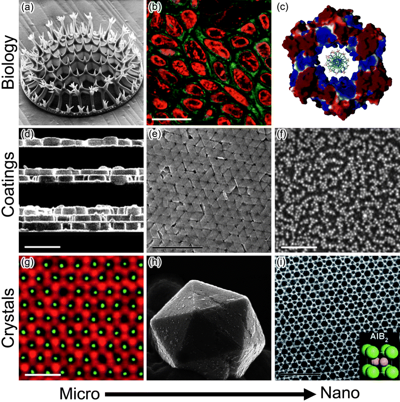 | ||
| Fig. 1 Electrostatics in various systems/applications at micro- and nanoscales. (a–c) Biological examples include (a)biomineralization of charged inorganic/organic species (here, a fragment of a micro-organism called a diatom grown through the biomineralization of charged organosilicates; reprinted with permission from ref. 237), (b) cellular uptake of charged nanoparticles which is dependent on both charge polarity and magnitude (here, NPs located in the cytosol are functionalized with green fluorescent groups and NPs in the cell nuclei are functionalized with red fluorescent groups; scale bar is 20 μm; reprinted with permission from Elsevier, ref. 238) and (c) how surface potential within regions of a protein influences functionality. Shown here is the DNA binding β subunit from E. coliDNA polymerase III. Blue and red colors denote regions of positive and negative surface potential, respectively; the positive charge at the center of the protein facilitates DNA complexation. Reprinted with permission from AAAS, ref. 239. (d–f) Electrostatics is also a useful in assembling surface coatings. Examples include (d) the so-called layer-by-layer assembly (shown here are cross-sectional views of zeolite crystals assembled between polyelectrolyte layers on glass substrates; one, two and three zeolite layers are shown; scale bar is 1 μm; reprinted with permission from ref. 240; Copyright 2001 American Chemical Society), (e) the use of repulsive electrostatic interactions to drive crystallization of Raman-active, close-packed mono and multilayers of gold nanotriangles (scale bar is 1 μm; reprinted with permission from ref. 105; Copyright Wiley-VCH Verlag GmbH & Co. KGaA, 2010) and (f) the deposition of densely packed films incorporating negatively and positively charged NPs (scale bar is 100 nm; reprinted with permission from ref. 200; Copyright 2001 American Chemical Society). (g–i) Electrostatics also provides a versatile route to materials with crystalline ordering (g) Binary crystals of fluorescent charged microparticles (scale bar is 10 μm; Reprinted by permission from Macmillan Publishers Ltd: Nature Materials,30 copyright 2003), (h) three dimensional crystals of oppositely-charged metal nanoparticles (reprinted with permission from ref. 169, Copyright Wiley-VCH Verlag GmbH & Co. KGaA, 2009) and (i) one of various binary nanoparticle superlattices (scale bar is 40 nm; Reprinted by permission from Macmillan Publishers Ltd: Nature Materials,32 copyright 2006). | ||
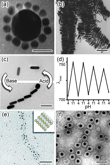 | ||
| Fig. 2 Nanoparticle structures assembled using various charged biomolecules. Complimentary strands of DNA direct assembly of (a) spherical nanoparticles (reprinted with permission from ref. 241; Copyright 1998 American Chemical Society) or (b) rods (ref. 242; Reproduced by permission of The Royal Society of Chemistry). Scale bars are, respectively, 20 nm and 100 nm. (c) Reversible assembly of nanorods has also been achieved through the use of a conformational change in a pH responsive polypeptide, poly(L-glutamaic acid). Scale bar is 50 nm. (d) The assembly/disassembly cycles are monitored by the shifts in the position of the rods' longitudinal plasmon resonance. Reprinted with permission from ref. 46; Copyright 2008 IOP Publishing. (e) Charged strands of DNA have also been used to template the electrostatic assembly of nanoparticles into linear strands or bundles (as shown here). Scale bar is 25 nm. Reprinted by permission from Macmillan Publishers Ltd: Nature Materials,94 copyright 2003. (f)Brome mosaic virus adsorbs onto NP surface via electrostatic attraction, and subsequently crystallizes into a capsid forming a ‘virus like particle’. Scale bar is 50 nm. Reprinted with permission from ref. 243; Copyright 2006 American Chemical Society. | ||
Electrostatic interactions between and assembly of charged NPs have been studied for a wide variety of particle shapes, including uniformly sized spheres,28 cubes,97 tetrahedra,33,98 rods,99 triangles,99 as well as mixtures containing spheres with different diameters63 and also mixtures of two differently shaped NPs.99 The electrostatic effects underlying these assemblies derive from charged or dipolar functionalities within the self-assembled monolayers88,100–102 (SAMs) which coat the particles. For interacting spheres, electrostatic forces mediate the formation of disordered aggregates or crystalline structures whose internal ordering depends on the charges32 and sizes of the particles,63 as well as the screening length.28,30,32 In all cases, the observed crystal structures correspond to a minimum-energy configuration of the NPs.28,30,32,103 Of course, electrostatic assembly methods are not limited to spheres. For instance, when nanocubes have zero, two, four, or five of their six faces coated with ionic ligands, these faces on different cubes repel one another causing the particles to organize into, respectively, three dimensional crystals,97,104 flat sheets, linear chains, or doublets.97 Electrostatic forces can also mediate the assembly of nanoscopic plates into large crystalline superlatticies,105 can control mutual positions of charged particles with precision down to a few nanometers,99 or can determine interactions with larger systems including living cells (where charge on nanosized particles affects their toxicity106–108 and/or cellular uptake109–111).
There are two key components that determine electrostatic interactions in nanoparticulate systems. First is the charged molecules tethered onto the particle surface. Usually, these molecules form self-assembled monolayers – of thiols, disulfides, or dithiolanes on Au,112,113Ag,114–116Cu,117–120Pt,121Pd,121–124 or Ni125–127 NPs; of silanes on silica,128–131alumina128–131 or titania,132,133 of phosphoric134,135 or carboxylic135–137 acids on iron oxides, etc. While the chemistry of SAMs and the use of specific charged groups (COO−, SO3−, PO3−, N(CH3)3+) have been reviewed in detail elsewhere,102,138–140 it should be mentioned that charge within the monolayer can be adjusted by the use of neutral “diluting” ligands—in this way, the so-called mixed SAMs (mSAMs) can be prepared with their net surface-charge density, σ, controlled by the fraction of charged molecules (for recent reviews of mSAMs, the reader is directed to141,142). In some interesting mSAM systems, the charged and uncharged thiols phase-separate to give “striped” nanoparticles—such inhomogeneous charge distributions lead to unusual forms of interparticle potentials (see ref. 143 and references therein).
The second way to control electrostatic effects in NP systems is through the electrostatic double layer (EDL) surrounding the particles. The EDL is comprised of solvent molecules and ions that are attracted to the charged surface, generally resulting in a locally increased concentration of counterions and decreased concentration of coions relative to their bulk-solution values. Importantly, the thickness of the EDL determines the range of electrostatic interactions in solution. The increased counterion and decreased coion concentration surrounding the particle causes the potential around the particle to decay exponentially with a characteristic length scale κ−1 (the Debye screening length). As more ions are added to the solution surrounding the NP, the value of κ−1 decreases so that the NPs need to be closer to one another in order to interact electrostatically.
Several theoretical models describing the EDL have been developed over the last 150 years, with their focus mainly on describing the interactions in colloidal systems. In an early model, Helmholtz144 described the EDL as a monolayer of counterions on a charged surface. Later, Gouy145,146 and Chapman147 treated the EDL as a diffuse charged layer near a charged surface – this approach led to the so-called Poisson–Boltzmann equation, which we discuss in detail later in this Review. These fundamental continuum models have been refined to include the effects of counterion size, changes in the dielectric constant, and image charges; they have also been simplified into more analytically tractable forms that can be used to describe interactions between particles of various shapes, sizes, and compositions.
We will begin this Review by a detailed discussion of models describing the EDL. Since our focus is on nanoscopic systems, we will pay special attention to the fact that in this regime, the size of the counter or coions can be within an order of magnitude of the charged nano-object itself. A question that naturally arises is then whether the ions can be treated by the continuum formalism of partial differential equations (in particular, Poisson–Boltzmann) or does the description of the EDL need to account for the ions' discreet nature. Once we address these issues, we will then turn our attention to the theoretical description of the boundary between the nano-object and its ionic atmosphere. With these preliminaries, we will be in position to develop interaction potentials acting between charged objects of different shapes and sizes and will be able to rationalize electrostatic phenomena behind the experimental, nanoscale systems discussed in Section 4. Although this Review will certainly not be a complete survey of nanoscale electrostatics, we hope it will provide a comprehensive background and methodology to allow the readers to derive basic formulas describing their own systems of charged nano-objects.
2. Models of the electrostatic double layer
Generally, models of the EDL aim at determining the spatial concentration profiles/distributions of ions surrounding a charged object. These distributions can be determined by a number of different routes, including Monte Carlo (MC) or molecular dynamics (MD) simulations, integral equations and statistical mechanical models, or continuum descriptions of the local ion concentrations. What is important to remember is that each type of calculation has its advantages and limitations. The MD/MC simulations and statistical models can be easily formulated to account for large numbers of interionic interactions, but they are limited by computational resources and can treat only relatively small systems. Continuum descriptions can be analyzed either analytically or numerically, but they discount the finite-size nature of the ions and many of the intermolecular interactions that appear in other models.2.1 Molecular-level descriptions of the electrostatic double layer
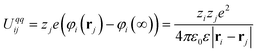
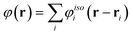
At the molecular level, the distribution of ions within the EDL can be studied by either MD or MC methods with ion–ion interactions taken into account explicitly. Most commonly, either the so-called restricted primitive model (RPM) or the mean spherical approximation (MSA), are used. In RPM, the charged species (the NP and the ions surrounding it) are treated as hard-sphere objects that interact with one another via long-ranged interactions (i.e., full Coulombic interactions) through a “continuum” solvent characterized by a uniform dielectric constant. The MSA retains the formulation of hard-sphere interactions between charged species from the RPM, but simplifies the long range interactions by linearizing the electrostatics. An offshoot of the MSA model is the MSA-HNC model (MSA with hypernetted-chain) which retains the hard-sphere interactions, improves the accuracy of the long range interactions by including non-linear electrostatics, and also accounts for short range interactions (i.e., van der Waals forces). It should be remembered that the MSA linearization of the electrostatic interactions is a simplification that underestimates the interactions between highly charged particles and can give unphysical values for the ion distribution functions around a NP; hence the MSA-HNC is preferable under these circumstances.The potential generated by an isolated charged particle at location ri is 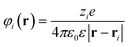 and the electrostatic potential energy required to bring an additional charged particle, labeled j and of charge zje, from infinitely far away to a position rj is given by
 | (1) |
 | (2) |
 | (3) |
Of course, charge-charge interactions are not the only electrostatic interactions that can affect NPs. The restricted primitive and MSA models neglect contributions due to induced electrical polarization of the NPs, ions and solvent, and also any permanent dipoles that may reside on the molecules comprising the solvent, both of which can significantly affect the distribution of ions around a NP. One way to account for polarization is to assign each NP, ion, and solvent molecule a dipole moment p, that may be permanent (as in water), or induced (for example, by the electric field generated by the NP and EDL). The energetic contribution of these dipoles may be included by introducing the terms:
 | (4) |
The above expressions are only strictly valid in the case of a uniform dielectric constant. This assumption, however, is virtually never valid in systems of charged nanoparticles, where the dielectric constant of NP cores ranges from ε ≈ ∞ (metallic NPs) to ε ∼ 2 to 4 (polymeric NPs) while the surrounding solvents have dielectric constants ranging from ε = 80.1 (water) to ε ∼ 2 (alkanes).148 Therefore, the electrostatic interactions around the NP surface are effectively weighted by a mean dielectric constant. In the limit of strongly charged NP surfaces this dielectric renormalization can cause large charge accumulation of counterions in the EDL which further decrease the dielectric constant around the NP with respect to the value of the solvent at infinite distance.
If the dielectric constant varies, the potential must satisfy Poisson's equation of the form ∇·(ε(r)∇φ(r)) = −ρ(r)/ε0 which relates the potential to the charge density, ρ, and dielectric constant, ε. Several methods have been developed to mathematically account for the variations in dielectric constant, as shown in Fig. 3, including the point-inducible dipole and local dielectric constant models for the entire system,149 and application of the method of images for systems with isolated regions of non-uniform dielectric constant.150 Finally, we note the most accurate simulations of EDL also take into account van der Waals dispersion forces and also magnetic dipole moments, both of which can also be expressed as sums of pairwise interactions.
 | ||
| Fig. 3 Illustrations of various models used in defining the dielectric constant. The dielectric environment can be (a) constant across the entire region of interest (including inside any particles), (b) constant within defined local regions, (c) a continuous moving average across a region defined by external parameters (e.g., local particle concentration), or (d) approximated by a series of well defined point dipoles. | ||
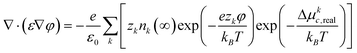
What are the key results of the EDL simulations? In most cases, these methods yield distributions of counterions around charged objects similar to those predicted by continuum models (to be discussed in the next Section). Of course, there are notable exceptions which arise when the NP is either highly charged (when σ > e/![[small script l]](https://www.rsc.org/images/entities/char_e146.gif) 2B, where B is the Bjerrum length discussed in Section 2.2; this corresponds to σ > 0.33 C m−2 for monovalent ions in water at 25 °C), for which MC simulations predict clustering or layering of the surrounding counterions,151 or when the asymmetry in the size of the ions present in the EDL is significant enough that correlation functions describing the distributions of counterions and coions exhibit characteristic oscillations.151–153 Such oscillations are illustrated in Fig. 4c, which has the MSA-HNC154,155 radial ionic concentrations for both coions (red lines) and counterions (blue lines) around a nanoparticle. For comparison, the monotonic dependencies from a simple continuum model are also shown – while this continuum model can account for size asymmetry of co/counterions, it fails to describe properly the forces between the ions.
2B, where B is the Bjerrum length discussed in Section 2.2; this corresponds to σ > 0.33 C m−2 for monovalent ions in water at 25 °C), for which MC simulations predict clustering or layering of the surrounding counterions,151 or when the asymmetry in the size of the ions present in the EDL is significant enough that correlation functions describing the distributions of counterions and coions exhibit characteristic oscillations.151–153 Such oscillations are illustrated in Fig. 4c, which has the MSA-HNC154,155 radial ionic concentrations for both coions (red lines) and counterions (blue lines) around a nanoparticle. For comparison, the monotonic dependencies from a simple continuum model are also shown – while this continuum model can account for size asymmetry of co/counterions, it fails to describe properly the forces between the ions.
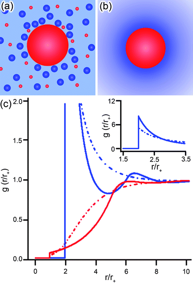 | ||
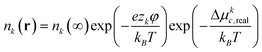
| Fig. 4 Schematic representations of a positively charged NP (red) surrounded by charged counter/coions (blue/red) from two different theoretical perspectives. (a) The primitive model, PM, and mean spherical approximation, MSA, treat the NP and surrounding ions as hard spheres with the solvent as a continuum. (b) The PB models simplify the theoretical description by treating both solvent and ions as continuous distributions. (c) The radial distribution functions, g, of anions (blue, of radius r− = 0.425 nm) and cations (red, of radius r+ = 0.2125 nm) around a positive NP (rNP = 1.5 nm, q = 36) as functions of the distance from the particle surface normalized with respect to the cation radius, r/r+. The MSA/HNC model (solid lines, corresponds to diagram in (a)) shows an “oscillatory” behavior while the non-linear PB model with size-asymmetric ions (dashed lines, corresponds to diagram in (b)) predicts a monotonic behavior. Inset shows region not in view of the main graph. | ||
We note that for an infinitely dilute system of charged nanoparticles it has been shown that the ionic size asymmetry in monovalent electrolytes can promote an unequal charge neutralization (i.e., ions of various sizes have different ‘efficiencies’ at screening charge) resulting in either charge inversion or charge amplification.151,156,157 In such systems, charge inversion occurs when the native colloidal/nanoparticle charge is overcompensated at certain distances within the EDL by small counterions which adsorb on the NPs surface and screen charge more effectively than the larger counterions. Charge amplification occurs when the size-asymmetry of the surrounding ions causes more like-charged coions to be present around the particle or when a weakly charged nanoparticle adsorbs like-charged ions on its surface via other attractive interactions (i.e., van der Waals interactions). Because continuum models based on PB equation do not account for many of these inter-ionic interactions, they rarely are able to predict the occurrence of these types of phenomena.156–158 As a result, other theories which rely upon the PB equation also fail when there are strong electrostatic interactions between counterions residing close to a particle surface.159–161 These inter-ionic correlations can be circumvented by using afore mentioned methods or by using density functional theories for nanoparticles.162
2.2 Continuum models of electrostatic interactions
The key difference between the continuum models and the discrete models discussed above is that instead of each charged molecule being addressed individually, only the average concentration of each species is determined at each point in the simulation. In order to apply the tools of thermodynamics, it is necessary to assume that the EDLs surrounding the NPs have equilibrated with any externally applied fields and are in their thermodynamically favored state. This means that the electrochemical potential of each species present in the system must be constant throughout this system—this simple fact provides the necessary foundation from which analytical models for the EDL may be developed.Since the energy of the system is a sum of electrostatic and non-electrostatic contributions (e.g., hard sphere, van der Waals interactions, and dispersion forces due to the solvent), the changes of chemical potential from a reference state may be written as
| Δμke = Δμkc + Δμkes | (5) |
| Δμke = kBTln(nk(r)/nk(∞)) + zke(φ(r) − φ(∞)) + Δμkc,real | (6) |
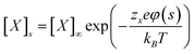
From this expression, it is possible to determine the system-wide distribution of each ion by setting Δμke = 0, which means that the electrochemical potential for each species is constant throughout the system (i.e., the ions near the NP surface are in equilibrium with the bulk ions in the electrolyte) and applying the commonly used approximation that φ(∞) = 0; this procedure gives:
 | (7) |
Multiplying nk by the charge per ion, ezk, gives charge density, ρ, that can be substituted into the Poisson–Boltzmann equation, ∇·(ε∇φ) = −ρ/ε0, to give:
 | (8) |
Various sets of assumptions about the ion-ion and ion-particle interactions can be input into eqn (8), which serves as a basis for the most commonly used EDL theories that are derived from the PB equation. When the ions in the system are treated as ideal point charges, ε is constant in each phase (for instance, a NP core has ε(r) = ε1, the ligands in the SAM have ε(r) = ε2, and the solvent has ε(r) = ε3 – each area is a separate phase in terms of how the PB equation is applied) and the electrolyte is “symmetric” (that is, z(+) = −z(−) = z and n(+)(∞) = n(−)(∞) = n∞), two important values can be introduced, the dimensionless potential, ψ = zeφ/kBT, and the Debye screening length, κ−1 = (kBTε0ε/2e2z2n∞)1/2, so that:
 | (9) |
which is the most common formulation of the Poisson Boltzmann equation. Due to the nonlinearity introduced by the sinh term, it is difficult to integrate this equation analytically, and, unlike the MD and MC models above, the potentials from multiple charged NPs cannot be superimposed which means that the PB equation must be solved for every change of systemic variables. These difficulties, however, can be circumvented by using a linearized form of eqn (8):
 | (10) |
On the other hand, it should be emphasized that linearized PB equation cannot be used to model strongly charged systems, mainly because in such cases the ions around the NP cannot be treated as non-interacting and their correlations should be taken into account (see Section 2.1). The key quantity to be considered is then so-called Bjerrum length, B = e2/4πεoεrkBT, which is the distance at which the electrostatic potential energy of two elementary charges e in a solvent with a relative dielectric constant εr is comparable to the thermal energy kBT. The corollary is that if two oppositely charged ions are within a distance lB, they pair-up to decrease the electrostatic energy at the expense of entropy (thermal energy) they would gain if they were dissociated. Due to the high concentration of ions around a strongly charged nano-object, the local dielectric constant is low and the Bjerrum length can be over 1 nm indicating that the ions have a tendency to “pair up” and cannot be treated as independent.
Many extensions and corrections to the PB equation have been developed to estimate various effects that produce increasingly complex equations and generally provide a better fit to experimental data. For example, if hard-sphere interactions are considered between the electrolyte and the NPs, then the first layer of ions interacting with a charged surface cannot be adsorbed directly onto the surface and, instead, they are separated from the surface by one ionic radii. When all ions have the same size, this is represented by the so-called Stern model:164,165
 | (11) |
 | (12) |
These more detailed descriptions of the double layers around charged particles can predict phenomena such as overcharging of nanoparticles151 and are more appropriate for highly charged surfaces. They also provide a good first approximation for the potential when the size asymmetry between counter- and coions is large without requiring the additional computations via molecular-level models.
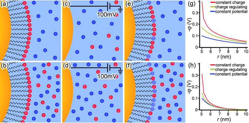 | ||
| Fig. 5 Illustration of the three types of boundary conditions applied to PB model of a spherical NP. The constant-charge boundary condition in (a,b) keeps the charged density on the NP surface constant, regardless of (a) low or (b) high concentration of ions surrounding the particle. The constant-potential boundary in (c,d) fixes the surface potential of the NP and is, strictly speaking, appropriate only for “bare” nano-objects serving as electrodes. Finally, the charge-regulating boundary condition in (e,f) is much more dynamic in that neither the surface charge density nor the surface potential are kept constant, but rather remain functions of the ion concentration surrounding the particle by coupling a mass balance equation (which describes the number of ions on the NP surface which are disassociated and have a net charge) with the PB equation. Plots of each boundary condition under (g) low and (h) high ion concentration show the differences in potential profiles around the NP (rNP = 5 nm). | ||
2.3 Boundary conditions
As for every partial differential equation, the PB equation requires the boundary conditions to be specified. The most important of these conditions—one reflecting the nature of the charged nano-object—is at the particle/solution interface and accounts for the way in which the particle acquires charge in solution through, typically, the dissociation of counterions. As in all other electrostatic systems, the potential at the NP/solvent interface must be continuous, φin = φout, and Gauss's law must be satisfied, (εin∇φin − εout∇φout)·n = σ/ε0, where n is the outward normal to the interface, and the superscripts in and out denote the particle and solvent, respectively. While the potential is calculated, and the dielectric constant specified, the surface charge density, σ, remains to be defined. In most systems of charged NPs, a dissociable group is exposed on the surface of a self-assembled monolayer, SAM, stabilizing the particle. The dissociation of ionizable groups in a SAM, AB ⇄ A± + B∓, is characterized by the equilibrium constant Kd = 1/Kb = [A±][B∓]/[AB], where Kd is the dissociation constant and Kb is the association/binding constant. If the molecules comprising the SAM were free in solution, the dissociation of each individual molecule would not affect other molecules. However, when the dissociable molecules are tethered onto a surface, the dissociation of each molecule causes a subsequent increase in the potential of the nearby molecules (if their cationic portions remain adsorbed; as in SAMs of alkane thiols terminated in –N(CH3)3+), or a decrease in the potential (if the anionic portions of the molecules remain adsorbed; as in SAMs of alkane thiols terminated in –COO−). This interplay between potential and association/dissociation of the ligands and ions from solution causes this form of boundary to be known commonly as a “charge-regulating” boundary condition.166,167In order to calculate the value of σ from the equilibrium between neutral and dissociated molecules on the NPs, the number of molecules per unit area, Γ, is multiplied by the average number of charges per molecule, γ, so that σ = Γγ. The value of Γ is constant for flat surfaces and is equal to the surface density of ligands in the SAM. For curved surfaces (e.g., cylinders or spheres), however, Γ depends not only on the surface density but also on the radius of curvature and the length of the molecules forming the SAM (see Fig. 9a, and Section 4.1.2 for further discussion). For example, Γ on the outer surface of a 5 nm diameter particle coated with a 1 nm thick SAM decreases to ∼51% of its flat surface value, while the same thickness SAM on a 100 nm diameter particle results in only a 4% decrease in Γ. The value of γ is determined by three factors (i) the value of Kd for the ions/ligands in solution, (ii) the concentration of ions in solution, and (iii) the potential at which the ligands are relative to the bulk of the solution. When the number of ions in solution is much greater than the number of ligands on the surface of the NPs (as is the typical case), then the concentration of ions infinitely far away is effectively constant, so the concentration of ions at the surface can be predicted using eqn (7) as:
 | (13) |
While the charge regulating boundary provides the most detailed description of the interaction between the ligands and ions in solution, there are two other commonly used approximations that are more mathematically tractable. The first is the constant charge condition, which occurs when the ligands retain the same charge regardless of potential—that is, no counterions or coions bind to the ligands and Kd is, strictly speaking, infinite (or at least very large as for very strongly acidic groups such as SO−3). The other limiting case that is commonly analyzed is the constant potential boundary condition, in which the potential of the surface is kept constant regardless of the concentration of electrolyte in the system. This boundary condition is most appropriate for a system that is connected to a potential source (i.e., a battery or an electrode)—for example unprotected NPs adsorbed onto an electrode. In terms of dispersed NPs, an approximation to this condition would require an infinite density of charged groups, with a Kd approaching zero, but a finite non-zero value of KdΓ.169 The three types of boundary conditions are illustrated in Fig. 5.
3. Energetics of the electrostatic interactions at the nanoscale
3.1 Energies of interaction between charged nanoparticles
Knowing the structure of the EDL and the appropriate boundary conditions sets the stage for calculating the free energies of interactions between charged nano-objects. In general, three distinct contributions to the free energy must be considered, (i) the potential energy due to electrostatic interactions, (ii) the entropic contribution from concentration of ions near the charged particle, and (iii) the chemical potential energy changes due to ion adsorption/desorption. The electrostatic potential energy is given in its typical form of: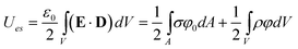 | (14) |
where the first integral is the energy as a function of the electric field, E, and the electric displacement, D. The second expression is a continuous version of eqn (3), with the first term accounting for the energy of the charged surfaces, and the second term accounting for the energy of the double layer surrounding these surfaces.
The entropic contribution in dilute solution is given by:170
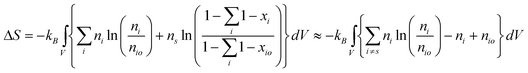 | (15) |
 | (16) |
Recognizing that the first term in the summation is similar to the charge density in the double layer, and applying an integral transformation, the entropic contribution can be written as:
 | (17) |
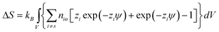
The free energy of the system (note that the Helmholtz and Gibbs free energies are identical if the ion distribution does not induce a change in solution volume) is then derived by the application of Green's formula and the addition of a progress variable (for details see Ref. 170):
 | (18) |
We note that this potential only accounts for the electrostatic portion of the free energy, and neglects any change in free energy due to the adsorption of ions at the charged interface. To include this energetic contribution after the formation of the monolayer, we use eqn (5), with Δμkc equal to the energy released when an ion dissociates or associates and Δμkes = zkeφsurf; at equilibrium, Δμkc = −zkeφsurf for each individual ion pair. In order to integrate this over the area, the surface charge density is used instead of zke, giving:167,170
 | (19) |
The overall change in free energy is then given by the sum:
 | (20) |
This result can also be derived using charging processes, or interaction forces.
The derived energy can be used to calculate the free energy of interaction between charged NPs. If the isolated particles are taken as a reference state, the free energy of interaction between N particles is given as:
| ΔG = Gsys − NGiso | (21) |
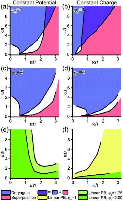 | ||
| Fig. 6 Phase diagrams depicting where either the Derjaguin or linear superposition approximations yields a force between two particles which deviates by less than 10% from the non-linear PB equation. Diagrams depict (a) constant potential or (b) constant charge boundary conditions where the dimensionless surface potential is φo = 1 and (c) constant potential or (d) constant charge boundary conditions where φo = 4. (e, f) Direct comparison between linearized and non-linear PB equation under either (e) constant potential or (f) constant charge boundary conditions at various values of dimensionless surface potential. The shaded regions represent conditions where the force between two nanoparticles calculated by linearized PB equation deviates by less than 10% from non-linear PB equation for surface potentials equal to or less then the indicated value. Plots are adapted with permission from Elsevier, ref. 176. | ||
3.2 Approximate expressions for energetic interactions
While eqn (18) will always give the free energy of the system, it is often not feasible to perform the integration over all surfaces/particles, especially in large systems (e.g., NP aggregates). It then becomes convenient—and, indeed, necessary—to introduce appropriate approximations, of which the so-called Derjaguin and linear-superposition (LSA) approximations are the most useful and popular.In the Derjaguin approximation,171–173 the interaction between non-planar particles is simplified by assuming that the interaction energy (or force) per unit area is the same as for infinite parallel plates. Specifically, the interacting curved particles are approximated as sets of infinitesimal parallel plates separated by a distance h′. The interaction energy is then calculated by multiplying the interaction energy per unit area for parallel plates, upp(h′), by the area of the curved surfaces at a given separation, A(h′), then integrating over all distances h′:
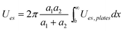
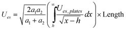
| U = ∫∞hupp(h′)A(h′)dh′ | (22) |
When applied to two interacting spheres,173 with radii a1 and a2, the Derjaguin approximation gives the interaction potential
 | (23) |
| Geometry | Potential | Boundary Condition | Range |
|---|---|---|---|
| Sphere/Sphere | U es = −2πεεoaφ2oln(1 − exp(−κh)) | Constant Charge |

|
| σ o = σo,1 = σo,2 | |||
| a = a1 = a2 | |||
| Sphere/Sphere | U es = 2πεεoaφ2oln(1 + exp(−κh)) | Constant Potential |

|
| φ o = φo,1 = φo,2 | |||
| a = a1 = a2 | |||
| Sphere/Sphere | U es = 2πεεoaφ2o exp(−κh) | Constant Charge or Constant Potential |

|
| a = a1 = a2 | |||
| Plate/Plate |
|
Constant Charge | φ o ≤ 25 mV |
| σ o = σo,1 = σo,2 | |||
| Plate/Plate | U es = εεoκφ2o[1 − tanh(−κh/2)] | Constant Potential | φ o ≤ 25 mV |
| φ o = φo,1 = φo,2 | |||
| Plate/Plate |
|
Constant Potential | φ o ≤ 25 mV |
| φ o,1 ≠ φo,2 | |||
| Sphere/Sphere |
|
Given by Ues,plates | Any from Ues,plates |
| a 1 ≠ a2 | |||
| Cylinder/Cylinder (Side-to-Side) |
|
Given by Ues,plates | Any from Ues,plates |
| Cylinder/Cylinder (Crossed) |

|
Given by Ues,plates | Any from Ues,plates |
| Cylinder/Sphere |

|
Given by Ues,plates | Any from Ues,plates |
| Plate/Sphere |

|
Given by Ues,plates | Any from Ues,plates |
In LSA, it is assumed that the potential of the entire system may be written as a sum of the potentials of isolated particles:
 | (24) |
These approximations have been compared to exact integrations for both the linearized174,175 and nonlinear176 PB equations for interacting spheres in terms of dimensionless diameters, κa, and κh, where a is the NP radius and h is the distance between the charged surfaces of the NPs. As shown in Fig. 6, the Derjaguin approximation for the force between two spheres is generally within 10% of the exact nonlinear PB solution for small separations and κa > 2, while it entails more than 10% error when used for smaller κa values. To understand these comparisons in terms of actual physical dimensions and concentrations, we note that if two 5 nm diameter spheres are interacting, the Derjaguin approximation would be valid if the concentration of a symmetric monovalent electrolyte surrounding them were ∼60 mM or greater.
The Derjaguin approximation is very useful because the nonlinear PB equation can be solved in a closed form between parallel plates. This allows for the force or interaction energy between two nano-objects to be expressed in a closed form as well – that is, a reasonably accurate estimation of the forces/energies can be made without using more complicated numerical techniques. On the other hand, when the particles are far apart, the LSA provides a better estimate than the Derjaguin formalism. This is so because, as the distance from a nano-object increases, the values of φ and ∂φ/∂r both decrease to zero. Thus, if one were to calculate the energetic change of a system of NPs using these approximations, the LSA should be used for the particles being far apart, while the Derjaguin approximation should be used for more closely spaced particles.
The linearized PB equation is, as expected, more accurate for lower potentials in both the constant-charge and constant-potential situations. Interestingly, this approximation is better for small separations in the constant potential case, and for large separations in the constant charge case; consequently, one must use caution when applying it to any charge-regulating systems.
While the numerical integration of both forms of the PB equation for interacting spheres is no longer a technical challenge, it is often convenient to use one of many analytical approximations for the interaction between different objects. For instance, the free energy of two interacting spheres that are separated by a distance r > κ−1 can be written as:
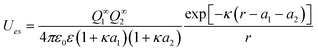 | (25) |
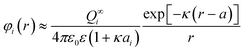 | (26) |
In the low potential limit, the renormalized charge is proportional to the surface charge density, Q∞i = 4πa2iσ∞i. At large surface potentials (φ ≈ 4kBT/e), the renormalized charge saturates, and can be estimated using eqn (26) as Q∞i = 4πε0εai(1 + κai)(4kBT/e). This has been further extended in the case of the linearized PB equation in both series and closed forms for spherical particles with different diameters and all possible combinations of constant charge, charge regulating, and constant potential boundary conditions.177 Similar approximations have been derived for interactions between spheres, plates and rods in multiple configurations as shown in Table 1, were a's denote radii of the interacting particles, and h is the separation between their surfaces
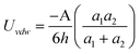
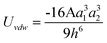
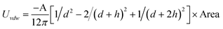
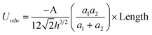
In real NP systems, these potentials are often considered in conjunction with attractive vdW interactions between the NPs (Table 2 lists potentials for some typical geometries). In this table the characteristic radius of the problem is a, the separation between the particle surfaces is h, and A is the Hamaker coefficient specific to the material/solvent system. This juxtaposition is the basis of the so called Derjaguin-Landau-Verwey-Overbeek, DLVO, theory,170,171,178–180 which yields total interaction potentials such as those illustrated in Fig. 7 for like-charged spherical particles.
![(a) Scheme of interacting NPs of radius ai and charge qi, whose surfaces are separated by distance h. (b) Plots of the magnitudes of electrostatic, Ues, and van der Waals, Uvdw, energies for NPs of charge q = 1e, 10e, and 100e as a function of NP radius, a, at a fixed separation of h = 2.8 nm (twice the thickness of a C12 SAM). (c) Electrostatic, van der Waals, and total energy profiles as a function of separation between two 10 nm NPs of charge q = 5e. Electrostatic forces are long-ranged compared to the van der Waals interactions that dominate at smaller separations (the separation distance due to the thickness of the SAMs is indicated by the vertical dashed line). The net energy barrier at a finite separation prevents particle aggregation. (d)Utotal profiles for NPs of various radii. All electrostatic interactions shown here are for the case of unscreened NPs ([Ions] = 0, κ−1 = ∞) of charge q = 15e. In all plots, the van der Waals interactions are calculated for Au NPs with water as the solvent (Hamaker constant, A = 9 × 10⁻²⁰J).](/image/article/2011/NR/c0nr00698j/c0nr00698j-f7.gif) | ||
| Fig. 7 (a) Scheme of interacting NPs of radius ai and charge qi, whose surfaces are separated by distance h. (b) Plots of the magnitudes of electrostatic, Ues, and van der Waals, Uvdw, energies for NPs of charge q = 1e, 10e, and 100e as a function of NP radius, a, at a fixed separation of h = 2.8 nm (twice the thickness of a C12 SAM). (c) Electrostatic, van der Waals, and total energy profiles as a function of separation between two 10 nm NPs of charge q = 5e. Electrostatic forces are long-ranged compared to the van der Waals interactions that dominate at smaller separations (the separation distance due to the thickness of the SAMs is indicated by the vertical dashed line). The net energy barrier at a finite separation prevents particle aggregation. (d)Utotal profiles for NPs of various radii. All electrostatic interactions shown here are for the case of unscreened NPs ([Ions] = 0, κ−1 = ∞) of charge q = 15e. In all plots, the van der Waals interactions are calculated for Au NPs with water as the solvent (Hamaker constant, A = 9 × 10⁻²⁰J). | ||
| Geometry | Potential | Range |
|---|---|---|
| Sphere/Sphere |
|
a 1,a2 ≫ h |
| Sphere/Sphere |
|
a 1,a2 ≪ h |
| Plate/Plate (semi-infinite) |

|
|
| Plate/Plate (finite thickness, d) |
|
|
| Cylinder/Cylinder (Side-to-Side) |
|
a 1,a2 ≫ h |
| Cylider/Cylinder (Side-to-Side) |
|
a 1,a2 ≪ h |
| Cylinder/Cylinder (Crossed) |
|
a 1,a2 ≫ h |
| Plate/Sphere |

|
a ≫ h |
| Plate/Sphere |

|
a ≪ h |
3.3 Limitations of pairwise continuum interactions
Although, as we have discussed, the Derjaguin approximation and LSA are good for many types of interparticle interactions, they become less accurate at small κa and κh, where the EDL thickness, particle size and particle separation are all of similar magnitude, which is especially relevant to charged nanoparticles. Also, as two particles approach one another, the EDLs around them merge causing the ions within the layers to redistribute around the entire particle as opposed to the local redistribution that occurs at large κa. When a third particle is introduced to the system, its interaction causes further adjustment of the EDL not only due to the distances between the individual particles (pairwise interactions), but also from contributions due to all three EDLs interacting (three-body interactions). In systems of like-charged particles, pairwise interactions (i.e., particles 1 and 2, 2 and 3, and 1 and 3) are all repulsive, however, recent experimental181–184 and theoretical183,185–187 work has shown that three-body interactions between like charged particles can be attractive in systems where κa ∼ 1. Conceptually, the addition of a third charged particle screens the interaction between the other two, thus making the three-body contribution energetically favorable. Interestingly, both two- and three-body interactions in nonlinear PB systems can be well approximated by the so-called Yukawa potentials.185 The two-body interactions are represented as U = A2 exp(−κr)/r, while the three- body interactions scale as U = −A3 exp(−γL)/L where L = r12 + r23 + r13 is the total distance between particle centers and the parameters A2, A3 and γ depend on the charge and the screening length of the system. While the pairwise and three-body interactions have the same profile, the total distance between particle centers in the three-body interactions will typically be longer than the pairwise interactions, so the energetic contribution of each three-body interaction will be less than each pairwise interaction; however, there are many more three-body interactions in close packed structures than two-body ones, so the overall energy of forming an extended structure can be favorable. It must be remembered though, that these undisputedly fascinating effects are still poorly understood and more fundamental work is needed before they can be used to explain formation of specific nanostructures.4. Nanoscale electrostatics in practice—key systems and experiments
Armed with the basic knowledge of the fundamentals of nanoscale electrostatics, we are now in position to review the recent studies involving charged nano-objects. We will begin by discussing the properties of individual charged nanoparticles, will then focus on the basic aspects of interparticle interactions, and will conclude with the discussion of large assemblies and materials comprised of charged NPs.4.1 Individual charged particles
 | (27) |
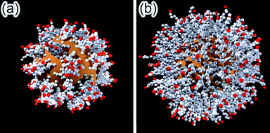 | ||
| Fig. 8 Monte Carlo simulation of spherical nanopartciles functionalized with ligands having hydrophobic tails terminated in (a) uncharged and (b) charged groups. In SAMs presenting charged end-groups, the ligands are more strateched out and form a more homogeneous monolayer. In both cases, the simulation accounts for 392 ligands, 10 monomers each, bound to a 5 nm particle (as in, for example, 5 nm AuNPs covered with alkane thiolates). | ||
When MC simulations are performed according to the Metropolis algorithm and with simulated annealing cooling schedule, the typical equilibrium configurations are such as those in Fig. 8. For the uncharged end-groups (Fig. 8a), the energy of the system is dominated by the hydrophobic interactions between the chains, which tend to bundle together and form “patches,” whose number depends strongly on the grafting density of the ligands as well as their chain length. On the other hand, when the end groups are charged (Fig. 8b), the electrostatic repulsions dominate – in particular, for relatively short chain lengths (6–12 monomeric units, corresponding to typical alkane thiolates used to stabilize nanoparticles), these repulsions prevent bundling and the ligands stretch out into the surrounding solvent maximizing the average distances between the charged groups and effectively rendering the SAMs more homogeneous. This relative homogeneity partly justifies the use of continuum models in which the charge density on the surface of NPs is, for a given particle size/curvature, treated as constant.
Of course, these intuitive arguments cannot substitute for a “real” theory. A notable – though relatively complex – theoretical treatment has been developed by Szleifer et al. and accounts for the free energies of acidic ligands as well as the surrounding counterions. We emphasize that the use of free energies rather than potential energies is necessary to model the equilibrium constants and, consequently, the pKa dependencies. In this approach,192–194 the free energy functional F, is written as a sum of several contributions, F = −TSmix − TSconf + Evdw + Erep + Eelec + Fchem, where T is the temperature, Smix is the mixing entropy of the mobile species (cations, anions, water, hydroxyl ions, and protons), Sconf is the conformational entropy of the grafted ligands, Evdw is the energy of the attractive van der Waals interactions, Erep accounts for the steric repulsive interactions between all the molecular species, Eelec is the total electrostatic energy, and Fchem represents the free energy associated with the acid–base chemical equilibrium, which is the free energy associated with the degree of protonation and deprotonation of the acid groups. While the mathematical details of this model are well beyond the scope current Review, it is worth noting that the model treats explicitly all possible conformations of the NP-grafted ligands and configurations of ions, and weights their energetic contributions according to the principles of statistical mechanics. This exhaustive treatment translates into a singular accuracy of this approach – the pKa trends predicted by the model (see solid lines in Fig. 9b) are in close agreement with experimental data.
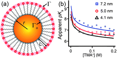 | ||
| Fig. 9 (a) Scheme of a nanoparticle or radius r covered with a SAM of charged ligands (of thickness L). The density of charged end-groups at the outermost surface of the SAM is Γ = Γo(r/r + L)2 where Γo is the density of binding sites for ligands on the NP (e.g., Γ0 ≈ 4.7 nm−2 for alkane thiols on Au190). (b) The apparent pKa of carboxylic acids bound to a NP surface is a function of the bulk ionic concentration of the surrounding solution, and also of the NP radius. Here, we see that a difference of ∼3 nm in the NP core diameter leads to a change of ∼1 pH unit in the pKa. Markers correspond to experimental data, lines are theoretical fits.248 | ||
![(a) Scheme of AuNPs functionalized with electron-rich TTF stalks (left) and bistable [2]rotaxanes (right). (b) Structural formulae of the ligands. (c,d)Cyclic voltammograms of ligands (c)2 and (d)34+ present free in solution and adsorbed on Au NPs at various surface concentrations, χ. (e,f) Experimental (×) and calculated (□) shifts in the redox potential, φ, of TTF in (e)1/2-Au NPs and (f)1/34+-Au NPs as a function of the surface coverage, χ. Blue and yellow traces correspond to the first and second oxidation potentials of TTF, respectively. Adapted with permission from ref. 168. Copyright 2010 American Chemical Society.](/image/article/2011/NR/c0nr00698j/c0nr00698j-f10.gif) | ||
| Fig. 10 (a) Scheme of AuNPs functionalized with electron-rich TTF stalks (left) and bistable [2]rotaxanes (right). (b) Structural formulae of the ligands. (c,d)Cyclic voltammograms of ligands (c)2 and (d)34+ present free in solution and adsorbed on Au NPs at various surface concentrations, χ. (e,f) Experimental (×) and calculated (□) shifts in the redox potential, φ, of TTF in (e)1/2-Au NPs and (f)1/34+-Au NPs as a function of the surface coverage, χ. Blue and yellow traces correspond to the first and second oxidation potentials of TTF, respectively. Adapted with permission from ref. 168. Copyright 2010 American Chemical Society. | ||
In the context of our discussion of nanoscale electrostatics it is important to note that these results can be quantified by relating the shifts in redox potential, E, to the changes in the electrostatic potential around the particles, φ. Two observations are relevant here: (i) that the oxidation of ligands X adsorbed on NP surfaces causes φ around the particle to increase and (ii) that the more of the oxidized species are already present on the surface, the more difficult it is to oxidize more of these groups and introduce additional charge onto the particle (negative electrostatic cooperativity). Based on these premises, it can be expected that the oxidation potential of adsorbed X is related to φ: to the first approximation, one can write Ex = E0 + φ, where Ex is the observed oxidation potential at the particle's surface (metal core plus SAM) and E0 is the oxidation potential of molecule X in a dilute solution. In other words, the shift in the oxidation potential Ex − E0 is equal to the electrostatic potential due to the immobilized ligands, φ. The value of the latter is found readily by solving the by-now familiar Poisson–Boltzmann equation, ∇2ψ = κ2sinh(ψ), where κ−1 is the Debye screening length, and ψ = eϕ/kT is the dimensionless potential. Importantly, the dependence of the potential on the surface concentration of the ligands, χ, and the curvature/radius of the nanoparticle, R, influences the solution to the problem via the boundary condition of the form  , where σ stands for the surface charge density on the NP. While other mathematical details can be found in ref. 195 and 168, the key point is that this relatively straightforward model predicts accurately – to within less than 5% – the changes in redox potentials for NPs of different sizes and functionalized with various types of redox-active molecules including structurally complex pseudorotaxanes, bistable [2]rotaxanes (Fig. 10e,f), or catenanes. Lastly, the model is generic in the sense that it can be easily adapted to other types of charged switches.
4.2 Aggregates of charged nanoparticles
Isolated charged nano-objects such as those described in previous Sections are an idealization and in real experiments the sample contains multiple particles. While the interactions between like-charged objects are typically strictly repulsive and incapable of bringing these particles together (but see Section 4.2.2 below), the mixtures of oppositely charged NPs appear naturally suited for the assembly of larger structures. We will first describe phenomena in which the charged NPs form either smaller and/or internally disordered aggregates—the assemblies and materials exhibiting long-range crystalline ordering will be described in Section 4.3.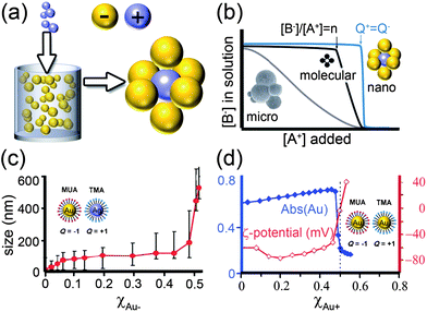 | ||
| Fig. 11 a) Scheme of the titration experiment in which a solution of negatively charged NPs (e.g., Au/SH-(CH2)11-COO−, MUA; yellow) is titrated with a solution containing positively charged NPs (e.g., Ag/SH-(CH2)11-N(CH3)3+, TMA; blue-gray). When a small number of positively charged NPs are added to a large number of negatively charged NPs, they form clusters whose negative surface charge stabilizes them in solution. b) The titrated nanoparticles precipitate from solution sharply only upon reaching the point of whereby the charges on the NPs are balanced. In contrast, molecular ions precipitate at the product of solubility, whereas oppositely charged colloids precipitate continuously. c) Average size of aggregates measured by DLS during titration of 11 nm AuMUAs with 11 nm AgTMAs. d) Intensity of the Au SPR band at λmax 520–550 nm (blue line) and the values of the ζ-potential (red line) for the titrations of oppositely charged, 5.5 nm AuNPs. Figure adapted with permission from ref. 190. Copyright 2006 American Chemical Society. | ||
Naturally, as the titration progresses, the oppositely charged NPs aggregate—this is evidenced both by the dynamic light scattering, DLS, data in Fig. 11c as well as the red-shifting of the particles' SPR band (blue curve in Fig. 11d). Surprisingly, however, the surface potential of the forming aggregates remains constant (red curve in Fig. 11d) despite the fact that the added/“minority” NPs have charge opposite to that of the “majority” particles originally present in solution. Only when the solution is about to precipitate, the magnitude of the potential decreases rapidly and is zero at the precipitation point (Fig. 11d). These findings—supported by UV-Vis spectroscopic analyses203 as well as theoretical considerations199,201—indicate that the NPs form aggregates whose outer shells contributing to surface potential are composed mostly of the “majority” particles (Fig. 11a). These shells render all aggregates like-charged and stabilize them in solution by mutual electrostatic repulsions. When the net charge on the NPs is close to neutral, there are not enough “excess” NPs to form like-charged shells, and precipitation ensues.
These results pose some interesting questions. Why, one might ask, are the NP clusters forming before the point of electroneutrality stable despite having net charge? And why, in the first place, is the sharp precipitation a nanoscale-specific phenomenon not seen with larger, microscopic particles?196–198 To answer these questions, we observe that the solutions of NPs before precipitation point are stable not only kinetically for a given period of time, but also thermodynamically (in experiment, for months). This property implies that NP aggregation can be explained based on the energies of interparticle interactions.
To calculate electrostatic interparticle interactions, we can use the formalism developed in Sections 2 and 3 to first solve for the electrostatic potential, φ, and then derive the free energy of interaction via the thermodynamic integration method described in detail in ref. 177, 178. Since the potentials around charged NPs are usually less than ∼50 mV, the linearized version of the Poisson–Boltzmann (PB) equation, ∇2φ = κ2φ, can be used together with the “charge-regulating” boundary conditions we discussed in Section 2.3. For the case of an individual NP coated with NT positively charged surface ligands, A+, in a solution containing negatively charged counterions, B−, the counterion dissociation equilibrium is determined by NA+CB−/NAB = K+ exp(eφs/kBT), where NA+ and NAB are, respectively, the numbers of counterion-free and counterion-bound surface ligands (NA+ + NAB = NT), CB– is the concentration of counterions in solution, K+ is the equilibrium constant in the absence of any external fields, and φs is the electrostatic potential at the NP's surface. From this relation, the surface charge density, σ, may be expressed as σ = eρ/[1 + (CB−/K+)exp(eφs/kBT)], where ρ = NT/4πR2 is the surface density of charged groups, and R is the NP radius. Assuming the dielectric constant of the NPs (εp ≈ 2 for the SAM coating) is small compared to that of the solvent (ε ≈ 80 for water), the surface charge is related to the potential at the NP surface by  , where
 ![[n with combining right harpoon above (vector)]](https://www.rsc.org/images/entities/i_char_006e_20d1.gif) is outward surface normal. Equating the two relations for σ provides the necessary boundary condition for a positively charged NP and allows us to solve for the equilibrium constant of the charged ligands; the case of a negatively charged particle may be derived in a similar fashion.
is outward surface normal. Equating the two relations for σ provides the necessary boundary condition for a positively charged NP and allows us to solve for the equilibrium constant of the charged ligands; the case of a negatively charged particle may be derived in a similar fashion.
Once the equilibrium constant of the charged ligands is known on a single NP, the linearized PB equation must be solved numerically in conjunction with the linearized charge regulating boundary conditions177 for the case of two interacting NPs. This process yields potential profiles which are used to calculate the interaction potentials in Fig. 12.
![(a,b) Electrostatic potential along the axis, x, connecting two (a) oppositely charged and (b) like charged NPs. Note that the potential is smaller between oppositely charged NPs, resulting in desorption of counterions and enhanced electrostatic attraction. The potential is larger between like-charged NPs, causing further adsorption of counterions and reduced electrostatic repulsion. (c) Magnitude of the electrostatic interaction energy, |ues|, between two oppositely charged and two like-charged NPs as a function of the distance between their centers, d. The dashed line is the approximate form ues(d) = 4πε0εφ2sR2exp[−κ(d − 2R1)]/d. Reprinted with permission from ref. 190. Copyright Wiley-VCH Verlag GmbH & Co. KGaA, 2007.](/image/article/2011/NR/c0nr00698j/c0nr00698j-f12.gif) | ||
| Fig. 12 (a,b) Electrostatic potential along the axis, x, connecting two (a) oppositely charged and (b) like charged NPs. Note that the potential is smaller between oppositely charged NPs, resulting in desorption of counterions and enhanced electrostatic attraction. The potential is larger between like-charged NPs, causing further adsorption of counterions and reduced electrostatic repulsion. (c) Magnitude of the electrostatic interaction energy, |ues|, between two oppositely charged and two like-charged NPs as a function of the distance between their centers, d. The dashed line is the approximate form ues(d) = 4πε0εφ2sR2exp[−κ(d − 2R1)]/d. Reprinted with permission from ref. 190. Copyright Wiley-VCH Verlag GmbH & Co. KGaA, 2007. | ||
The striking feature of these dependencies is that the attractive energy between oppositely charged NPs at contact is nearly twice that of like-charged NPs at the same distance. This effect is due to the desorption of bound ions from the NPs' surfaces in the regions of reduced electrostatic potential (cf. the equilibrium relation above). Specifically, when oppositely charged NPs approach one another, the magnitude of the potential in the region between them decreases (Fig. 12a) causing counterions to desorb. This desorption, in turn, increases the local charge density and the electrostatic interaction energy. In contrast, the magnitude of the potential between proximal, like-charged NPs is enhanced (Fig. 12b), causing further adsorption of counterions, decrease in the local charge density, and reduction of the electrostatic interaction energy. The differences in the like-charged and oppositely charged interaction potentials are of central importance in rationalizing the core-shell NP clusters observed in experiments (cf.Fig. 11a)—colloquially put, the like-charge repulsions are more effectively screened than opposite-charge attractions, and so the like-charged NPs can form the “shells” stabilizing the NP aggregates forming before the point of electroneutrality is reached.
An interesting corollary of the NPs' singular precipitation behavior is the ability to control precisely the fractions of charged ligands on NP surfaces. Here, one begins by preparing “standard” NPs—typically, noble-metal nanoparticles of known size and fully covered with alkane thiols terminated in a charged functionality. Since the area of the surface occupied by each thiol is known (e.g., 21.4 Å2 for Au204) the charge of the “standard” is readily calculated. Then, to read the unknown charge on nano-objects of a different type, the solution of the “unknowns” is titrated with that of the “standards,” and the precipitation point where ∑ QNP(+) + ∑ QNP(−) = 0 reports the charge on the former. The precision of this method is within ∼3%, and we have found it particularly useful in determining charges of NPs covered with mixed self-assembled monolayers (mSAMs) composed of charged and uncharged thiols. Fig. 13 illustrates this method applied to NPs covered with a mSAM of 11-mercaptoundecanol (HS(CH2)11OH; MUO) and 11-mercaptoundecanoic acid (HS(CH2)10COOH; MUA), in a molar ratio αsurf = cMUOsurf/cMUAsurf = x/y. Naively, one might expect that mSAM of such composition, can be prepared by simply soaking non-functionalized, “bare” NPs in a solution containing x moles of MUO and y moles of MUA. In reality, the surface composition obtained in this way almost certainly will not be x:y, since the equilibrium constants for the adsorption of different thiols are different (Fig. 13a). Instead, a series of solutions of different proportions of the two thiols (say αsol = 0,2,4,8,16, 32, …) are prepared and their pH adjusted to 11 to deprotonate all MUA's carboxylic groups. This solution is then titrated with like-sized NPs fully covered with positively charged TMA thiols and the positions of the precipitation points χPas a function of αsol are recorded. To determine equilibrium constants from these experiments, we note that the absorption equilibrium constant of each thiol onto AuNPs is given by KT = cTAu/cTsolcAu, where T = MUO or MUA, cTAu is the concentration of thiol adsorbed onto AuNPs, cTsol is the concentration of free thiol in solution, and cAu is the concentration of free adsorption sites on the surface of AuNPs. Because the mole fraction of MUA thiol on the surface can be written as ηMUA = 1/[1 + αsol(KMUO/KMUA)], the positions of precipitation points for different values of αsol are related by χPα = χP0·ηMUA/(1 + χP0·ηMUA − χP0), where χP0is the precipitation point of AuNPs soaked in pure MUA (αsol = 0). Therefore, the ratio of the equilibrium constants KMUO and KMUA can be determined from the slope of the dependence of 1/χPα on αsol: 1/χPα = 1/χP0 + (1/χP0 − 1)(KMUO/KMUA)αsol (Fig. 13c). Knowing the relative adsorption equilibrium constants, one can then easily prepare NPs of desired charges—such particles then constitute building blocks of “nanoionic” materials to be discussed later in Section 4.3.
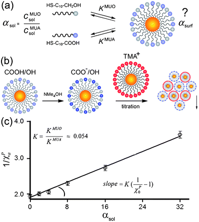 | ||
| Fig. 13 (a) The proportions of the MUA and MUO thiols in solution (αsol) and in the mixed SAM on the NPs (αsurf) are not equal. (b) To determine αsurf and the ratio of adsorption equilibrium constants, K, the MUA/MUO NPs are first deprotonated and then titrated with TMA NP “standards”. (c) The value of K is calculated from the slope of the dependence of 1/χPα on αsol. Reprinted with permission from ref. 190. Copyright Wiley-VCH Verlag GmbH & Co. KGaA, 2007. | ||
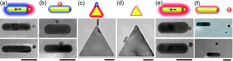 | ||
| Fig. 14 Site-selective electrostatic self-assembly of oppositely- and like-charged particles. Schemes and representative TEM images of (a, b) Oppositely charged nanoparticle/nanorod (NP/NR) systems. The “tip” arrangements shown in (a) is observed for large-screening length where charge-induced dipole interactions are appreciable (here, for TMA NPs/MUA NRs pair with κ−1≈ 10 nm). The “side” arrangement in (b) is observed for small screening lengths (TMA NPs/MUA NRs, κ−1≈ 0.6 nm). (c, d) Similar trends hold for nanotriangle/nanorod (NT/NR) systems (here TMA NTs/MUA NRs) with both (c) large and (d) small screening lengths. (e, f) Like-charged NP/NR systems. (e) for large screening lengths (here, TMA NPs/TMA NRs, cS ≈ 1 mM, κ−1≈ 10 nm) where charge-induced dipole attraction overcomes electrostatic repulsion, the particles aggregate in a “tip” arrangement; (f) when screening length is small (TMA NPs/TMA NRs, cS ≈ 250 mM, κ−1≈ 0.6 nm) and induced dipoles are negligible, repulsive electrostatic interactions dominate and the particles repel one another. In the schemes, the screening length is proportional to the thickness of the halos around the particles; red and blue colors indicate, respectively, positive and negative particle polarity. Scale bars for NR/NP and NT/NR systems are 20 nm and 50 nm, respectively. Reprinted with permission from ref. 99. Copyright 2010 American Chemical Society. | ||
An even more striking manifestation of the importance of the charge-induced dipole effects is illustrated in Fig. 14 e,f. Here, both the NPs and the NRs are like-charged. When the screening length is large, the charge induced dipole attraction actually overcomes the like-charge attraction and the particles aggregate in the “tip” configuration. When, however, the screening length is decreased (by the addition of salt), the charge-charge repulsion has the upper hand and the assembly falls apart.
A few comments are due regarding the theoretical treatment of electrostatics in systems of non-spherical particles. As might be expected, analytical solutions of the PB equation for such low-symmetry systems are difficult and in many cases prohibitive. Consequently, one can either resort to gross approximations—for instance, treat interacting particles as point charges and/or point dipoles (see ref. 99 for details)—or else use numerical packages such as COMSOL Multiphysics (previously known as FEM Lab) whereby the interacting objects are represented as a three-dimensional triangulated mesh (Fig. 15a) and the PB equation with appropriate boundary conditions is solved by the Finite Element Method.205FEM method is computationally intensive but can handle particles of any shape. It is important to remember, however, that while most software packages triangulate particle surfaces automatically, the quality of triangulation should be checked by the user to make sure that regions of higher curvature have finer mesh (this avoids the formation of sharp ‘edges’ in the mesh, which can prevent the convergence on a solution). When properly setup, FEM methods give solutions that have accuracy typically within a fraction of a per-cent from analytical ones (in problems where analytical solutions are available). An example of the results from such a calculation is shown in Fig. 15b, where an energy diagram is created for the NR/NP system discussed above. The energy of the system can be computed for the NP moving along the contour of the NR to show the configuration of lowest energy for each screening length.
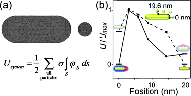 | ||
| Fig. 15 (a) Finite Element Method (FEM) can be used to solve for the potential around more complex geometries by representing these objects as a 3-dimensional mesh. After solving the PB equation with the appropriate boundary conditions (see Section 2.3) the surface potential can be numerically integrated over the surface and the energy of the system/configuration can be found. (b) Energy diagrams can be obtained from FEM calculations for various particle orientations and experimental conditions. Here, we show the normalized energy as a NP moves along the contour of a NR at either large or small screening lengths. As observed in the corresponding experiments (see Fig. 14), the FEM method predicts that a ‘tip’ assembly is preferred when the electrostatic interactions are unscreened, but the ‘side’ assembly becomes most favorable when the screening lengths are short. Reprinted with permission from ref. 99. Copyright 2010 American Chemical Society. | ||
4.3 Nanoscale self-assembly driven by electrostatic interactions
As we have seen in the previous Section, the nature (attractive/repulsive), the range and the directionality of electrostatic interactions at the nanoscale can be tailored by adjusting the shapes and sizes of the NPs as well as the characteristics of the surrounding medium. With such a flexible control, electrostatic forces are well suited to mediate assembly of nanostructured materials. In this section, we will review some recent examples of structures held by electrostatic forces, ranging from one dimensional chains to three-dimensional crystals and even crystals-within-crystals.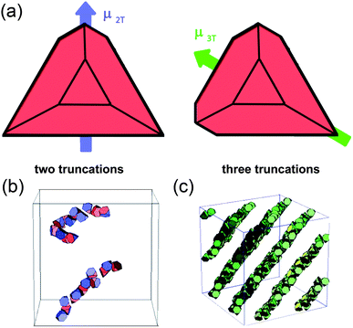 | ||
| Fig. 16 (a) The direction of dipole moments in tetrahedral CdTe nanoparticles with two and three truncations. (b, c) Computer simulations of the assembly of CdTe nanoparticles into (b) chains and (c) sheets. From ref. 207. Reprinted with permission of AAAS. | ||
The formation of “pearl-necklace” 1D assemblies illustrated in Fig. 16b depended crucially on the interplay between charge-charge repulsions and dipole–dipole attractions. In particular, these structures form only when some of the charged ligands are desorbed from CdTe surfaces such that the charge-charge repulsions are weakened. With careful control of this process, the dipole–dipole interactions remain significant and commensurate with charge-charge repulsions (both a few kT). The well-known preference of dipoles to align then leads to the formation of particle chains that can be up to 1μm long and exactly one nanoparticle wide.
The same CdTe nanoparticles but stabilized with positively charged DMAET rather than negatively charged TGA assemble into 2D sheets (Fig. 16c).33DMAET ligands have charges of magnitudes smaller than TGA and also bear methyl groups which contribute to attractive hydrophobic interactions between the NPs. The direction of the dipole, attractive hydrophobic interactions and repulsive electrostatic interactions between NPs then all contribute to the assembly of planar sheets. Calculations confirm that this type of assembly is the lowest-energy configuration characterized by antiparallel orientation of nearby dipoles, and is crucially dependent on the electrostatic effects. For instance, without electrostatic repulsions, the particles are predicted to form 3D aggregates with random arrangement of the CdTe components.
Referring a reader interested in mechanistic theoretical details to ref. 200, 211 we highlight some practical advantages of the method. First, since deposition leads to monolayers incorporating equal numbers of “+” and “−” NPs and is driven by the electrostatics alone (and not by the nature of the NPs' cores), it is possible to prepare the coatings made of different combinations of materials. For example, a solution of 25% of AuTMA NPs, 25% of AgTMA NPs and 50% of PdMUA NPs (TMA = SH-(CH2)11-N(CH3)3+; MUA = SH-(CH2)11-COO−) deposits a coating whose elemental composition is 1![[thin space (1/6-em)]](https://www.rsc.org/images/entities/char_2009.gif) :1:2 (see Fig. 17a for this and other examples). Second, because deposition is solution based, it can give uniform coatings over curved surfaces, including inner surfaces of vials and tubing. Fig. 17b shows examples of AgNP(+)/AgNP(−) coatings formed inside of Tygon tubing used in medical applications—owing to the bacteriostatic nature of silver nanoparticles, the tubing remains sterile in the presence of both Gram positive S. Aureus and Gram negative E. Coli bacteria.210 Finally, the ordering of the coatings can be improved by performing the deposition in the presence of AC fields that “jiggle” the charged particles and drive their close packing (Fig. 17c). The electrohydrodynamic phenomena accompanying AC forcing are described in detail in ref. 212.
:1:2 (see Fig. 17a for this and other examples). Second, because deposition is solution based, it can give uniform coatings over curved surfaces, including inner surfaces of vials and tubing. Fig. 17b shows examples of AgNP(+)/AgNP(−) coatings formed inside of Tygon tubing used in medical applications—owing to the bacteriostatic nature of silver nanoparticles, the tubing remains sterile in the presence of both Gram positive S. Aureus and Gram negative E. Coli bacteria.210 Finally, the ordering of the coatings can be improved by performing the deposition in the presence of AC fields that “jiggle” the charged particles and drive their close packing (Fig. 17c). The electrohydrodynamic phenomena accompanying AC forcing are described in detail in ref. 212.
 | ||
| Fig. 17 (a) SEM images (left panel) and XPS spectra showing structure and metal composition (right panel) of coatings composed of oppositely charged NPs having same or different metal cores: AgMUA/AgTMA (top), AuMUA/AgTMA (middle) and AuTMA/AgTMA/PdMUA (bottom). TMA = SH-(CH2)11-N(CH3)3+; MUA = SH-(CH2)11-COO−. (b) Examples of medically relevant components coated with bacteriostatic NP monolayers of oppositely charged nanoparticles: Tygon-R tubing, polypropylene micropipette tips, glass vials, and polypropylene syringes. Yellow-orange coatings are made of AgMUA/AgTMA; pink coatings, from AuMUA/AgTMA. Uncolored pieces are shown for reference. (c)SEM images of typical binary AuMUA/AgTMA NPs coatings deposited with different AC frequencies ranging from 100 to 800 kHz. All samples were prepared at the same electric field strength of 150 V cm−1 (i.e., 5 V across 340 μm) and 15 min of field application. Scale bars are 100 nm; the insets are 50 nm × 50 nm. Reprinted with permission from ref. 210. Copyright 2010 American Chemical Society. | ||
In their experiments, Shevchenko et al. used different combinations of metallic and semiconductor NPs (PbSe, PbS, Au, Ag, Pd, Fe2O3, CoPt3, and Bi) stabilized by the addition of different amounts of surfactants like oleic acid (OA) and tri-n-octylphosphine oxide (TOPO) that can modify the NPs surface charge. Electrophoretic mobility (μe) measurements without excess of any capping ligands demonstrated that these NPs have few fundamental charges each. The mobility distribution curve showed several distinct peaks corresponding to particle populations with −1, 0, 1 and 2 fundamental charges. However, by introducing an excess of TOPO and/or OA it was possible to prepare samples with NPs of precisely defined charge. While the mechanism behind this charge adjustment is not fully understood, it is an interesting illustration of controlling charges by means other than the ubiquitous self-assembled monolayers.
A case in point are PbSe NPs coated with oleate ligands, C17H33COO−, attaching to the Pb atoms on the particle's surface. When oleic acid is added to the solution in excess, some oleate species on the NP surface can be protonated and desorbed, leaving behind positively charged surface sites. The excess OA can also protonate the negatively charged oxidized Se sites (forming upon exposure to atmospheric oxygen), again increasing particle's net positive charge. In contrast, TOPO charges the NPs negatively, likely because of its ability to complex (positively charged) lead ions and abstract them from the NP surface, leaving behind an excess of negatively charged Se sites.
With charge magnitudes controlled to within one fundamental charge per nanoparticle, Shevchenko et al. were able to crystallize various BNSLs. For example (Fig. 18), 6.2 nm PbSe and 3.0 nm Pd nanoparticles formed orthorhombic AB- and AlB2-type lattices in the presence of oleic acid (under these conditions, metallic and semiconductor NPs were oppositely charged), while addition of TOPO caused the change of the BNSL structure to NaZn13-type (negative charge on metallic nanoparticles was neutralized by TOPO, and positively charged semiconductor nanoparticles became negatively charged).
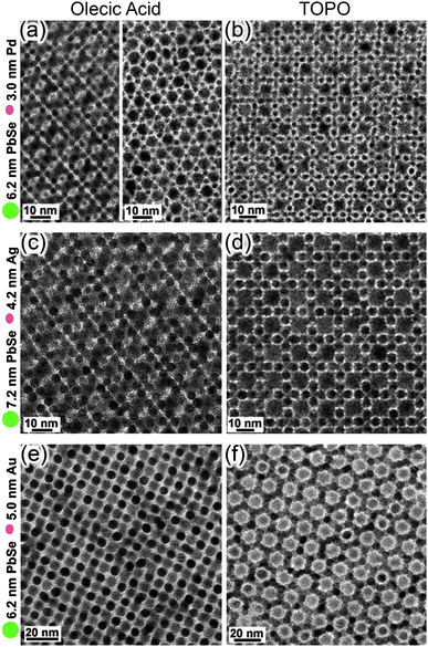 | ||
| Fig. 18 TEM images of BNSLs assembled in the presence of OA (left column) and TOPO (right column). (a) 6.2 nm PbSe and 3.0 nm Pd nanoparticles self-assembled into orthorhombic AB- and AlB2-type BNSLs in the presence of OA. (b) Same nanoparticles form NaZn13-type BNSL in the presence of TOPO(c, d) 7.2 nm PbSe and 4.2 nm Ag nanoparticles self-assembled into orthorhombic AB and cuboctahedral AB13 BNSLs, respectively. (e, f) 6.2 nm PbSe and 5.0 nm Au nanoparticles self-assembled into CuAu-type and CaCu5-type BNSLs, respectively. Reprinted by permission from Macmillian Publishers Ltd: Nature, 2006.32 | ||
It is worth mentioning that electrostatic interactions not only stabilize the superlattices, but also determine their stoichiometry. For the growth of large, ordered areas, the electroneutrality condition has to be fulfilled – that is, the positive charges should compensate the negative ones or else the local electrostatic energy of the lattice becomes unfavorable and further growth self-terminates. This was indeed seen in experiments showing relatively small regions of different types of BNSLs nucleating on the same substrate, but not exceeding 100 NPs, while stable structures with compensated charges comprised up to tens of millions of NPs.
Our work105 focused on the assembly of metallic nanotriangles, NTs, that are of particular interest due to the presence of sharp edges where electro-magnetic fields are concentrated into “hot-spots” which enhance SERS (Surface Enhanced Raman Spectroscopy) sensing abilities.219–223 In our experiments, the as-prepared NTs were stabilized by hexadecyltrimethylammonium bromide (CTAB). For these particles, crystallization protocol based on solvent evaporation led to disordered aggregates as illustrated in Fig. 19a. When, however, the NTs were functionalized with charged ligands such as N,N,N-trimethyl(11-mercaptoundecyl) ammonium chloride, TMA, they crystallized into large arrays several layers thick (Fig. 19b). Furthermore, when the charge on the NTs was further increased by intercalation of charged surfactants into charged SAMs, the triangles formed large-area monolayers (Fig. 19c).
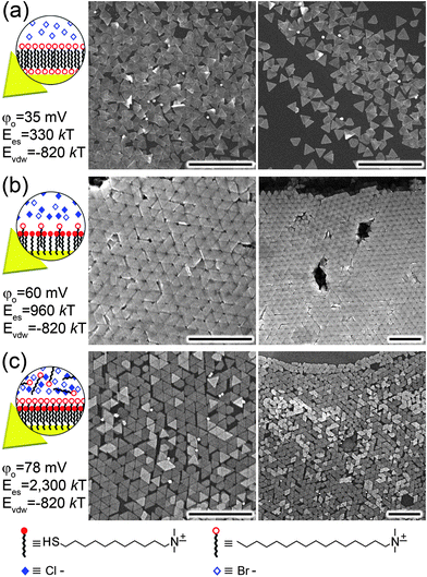 | ||
| Fig. 19 (a) Gold nanotriangles, AuNTs, stabilized only by excess cetyltrimethylammonium bromide (CTAB) surfactant (20 mM CTAB, surface potential φo = 35 mV, Eel ∼ 330 kT) form disordered aggregates. (b) Triangles functionalized with positively charged SAMs (here, of TMA thiols) and with only small quantities of CTAB surfactant present (<1 mM CTAB, φo = 60 mV, Eel ∼ 960 kT) organize into large, ordered multilayers. (c) AuNTs stabilized with TMA SAMs and in the presence of excess CTAB (20mM CTAB, φo = 79 mV, Eel ∼ 2,300 kT) give large monolayer arrays. All scale bars = 1 μm. Reprinted with permission from ref. 105. Copyright Wiley-VCH Verlag GmbH & Co. KGaA, 2010. | ||
While exact calculations of free energies (i.e., including entropic effects) for this system are prohibitively complicated, the experimental trends can be rationalized based on the interplay between van der Waals (vdW) attractions and electrostatic repulsions. The vdW forces increase with the area of contact and are the strongest when the NTs are stacked “on top” of one another. Approximating the triangles as semi-infinite plates of finite thickness, the energy of these interactions is EvdW = −A[1/d2 − 2/(d + h)2 + 1/(d + 2h)2]/12π,178 where A ∼ 10−19 J224 is the Hamaker constant for gold across water, d is the distance between the two plates (here, about two times SAM thickness, ∼2.8 nm28), and h ∼ 8.7 nm is the thickness of the plates (see Table 2). For the NTs we used, the maximal surface area of contact (when two triangles are stacked perfectly) is ∼11,000 nm2, and the corresponding Evdw ∼ −820 kT.
The vdW energies are partly offset by electrostatic repulsions. The electrostatic energy, per unit area, between two semi-infinite plates with equivalent potentials is225Eel = εεokφ2o(1 − tanh(kd/2)), where φois the constant potential at the plate's surface226 (see also Table 1). To determine φo, the by-now familiar linearized Poisson-Boltzman (PB) equation, ∇2φ = κ2φ, is solved with the relation between charge density and potential, σ = dφo/dx, applied at the boundaries x = 0 and x = d (coordinate x is perpendicular to the plates' surfaces). Solving yields σ = εκφo(coth(κd) − csch(κd)) which relates the surface potential to the charge density (determined from electrophoretic mobility experiments;227σ = μνκ,225 where μ is the mobility, ν is the viscosity of the medium, and κ−1 is the electrostatic screening length of a given solution). Once the surface potential of the particles is known, the electrostatic energy of the assembly can be calculated. For NTs stabilized by CTAB alone, the surface potential was measured at φo = 35 mV, and the calculated energy of electrostatic repulsion is Eel ∼ 330 kT. Since this energy is significantly smaller than Evdw, the process of assembly is dominated by vdW forces leading to rapid and indiscriminate aggregation. This situation changes for TMA-functionalized NTs for which φo = 60 mV and Eel ∼ 960 kT is commensurate with Evdw. In this case, the “balance” between electrostatic repulsions and the vdW attractions allows the NTs to adjust their mutual orientations during assembly leading to well-ordered, multilayer structures. Finally, when TMA SAM has extra charged surfactant intercalated, φo = 79 mV, and Eel ∼ 2,300 kT —then, the net interaction between the NTs is repulsive and the stacking of the NTs into multilayers is energetically unfavorable. At the same time, the triangles are large and massive enough that they sediment from solution onto the deposition substrate where they form monolayers.
The main and probably counterintuitive insight from these studies is that electrostatic repulsions can actually facilitate nanoscale self-assembly by softening strongly attractive interparticle potentials. It is a useful trick to remember!
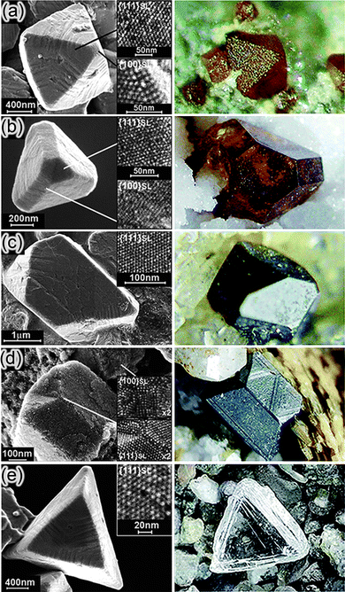 | ||
| Fig. 20 The left column has the SEM images of diamond-like crystals formed from oppositely charged, 5 nm Au and AgNPs. Insets zoom on the particles on the crystals' faces. The right column has the zinc-blend crystals (lattice isostructural with diamond) with similar morphologies. From ref. 28. Reprinted with permission of AAAS. | ||
While for equally sized and oppositely charged NPs one might expect – by analogy to inorganic ions – the crystal structure to be either NaCl or CsCl, nanoscale electrostatics again defies the intuitive. Surprisingly, the NPs crystallize into diamond-like structure, in which each NP is surrounded by four tetrahedrally arranged neighbors. Although in the diamond lattice each NP forms only n = 4 favorable “±” contacts (versus n = 6 in NaCl and n = 8 in CsCl), the like-charged particles in this open-lattice structure are farther apart than in the closed-packed NaCl or CsCl. Then, because the screening length around the NPs is commensurate with the particle diameters, the repulsions between like-charged next-nearest-neighbors in the diamond lattice are screened and effectively do not contribute to the unfavorable electrostatic energy of the crystal. Colloquially put, by “opening up” the structure one looses the favorable “±” energy, but saves on the “+/+” and “−/−” unfavorable contributions.
The sizes of the crystals can be controlled from several tens of nanometres up to several microns (see Fig. 21) by the addition of excess NPs of either polarity. The measurements of the ζ- potential indicate that the excess NPs “terminate” crystal growth by forming protective shells around the growing aggregates (see Section 4.2.1) – although the particles in these shells are all like-charged, the interactions between them are effectively screened, and the shells are stable.
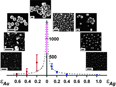 | ||
| Fig. 21 Size control during crystallization of equally sized, ∼5 nm AuMUA and AgTMA nanoparticles at pH 10. The graph plots average sizes (in nm) of crystals grown with different amounts of excess gold or silver NPs (εAu/εAg, respectively). Vertical bars denote the ranges of the crystals sizes observed; insets have the SEM images of typical crystals (scale bars are 100 nm for εAu = 0.6 and εAg = 0.2, 0.4, 1.0, and 1 μm for all other experiments). Dashed line is a theoretical fit to the expected d ∝ 1/εAg dependence. Reprinted with permission from ref. 249. Copyright 2007 American Chemical Society. | ||
It should be noted that crystallization of particles having different sizes and or charges remains problematic. In the former case, the NPs prefer to phase separate rather than co-crystallize. In the latter, the NPs often precipitate even if the charge ratios are small rational numbers – the reasons for this behavior are still not fully understood.
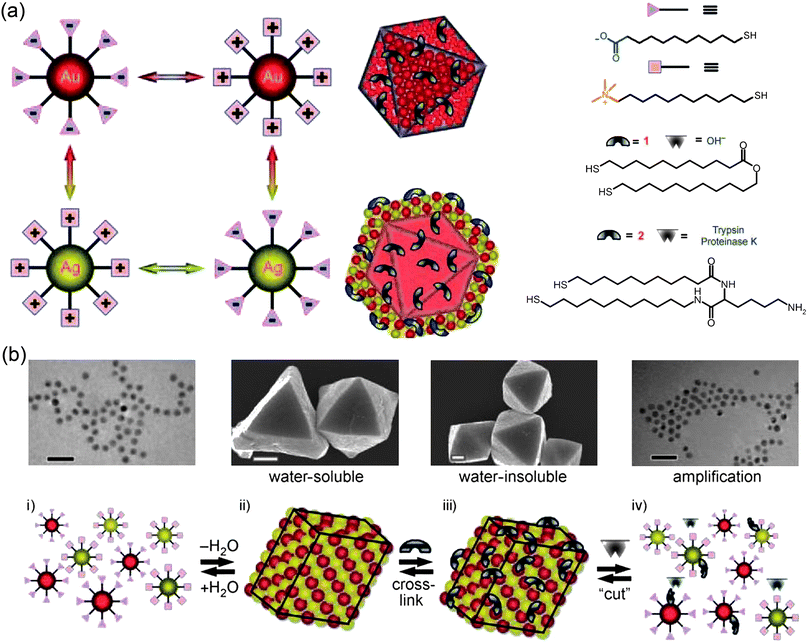 | ||
| Fig. 22 (a) Schematic representation of nanoparticles, crystals, and core-shell (“Russian Doll”) crystals used for amplified sensing. The fornulas on the right give the structures of the thiols coating the NPs, and also of two dithiols used to crosslink the crystals. One of the dithiols shown can be “cut” by hydroxyl ions; the other is cut by enzymes such as Trypsin or Proteinase K. (b) Procedure of amplified chemical sensing using nanoparticle supracrystals. Crystals self-assemble from oppositely charged NPs (i) and are soluble in water (ii). These crystals gain permanence and become water-insoluble when they are cross-linked with dithiols containing cleavable groups (see examples in a) (iii). When a specific analyte is added, the cross-links are chemically cut, and the crystals disintegrate into individual nanoparticles (iv). Reprinted with permission from ref. 228. Copyright Wiley-VCH Verlag GmbH & Co. KGaA, 2010. | ||
The same concept can be extended to “nanoionic” core-shell crystals. In this case, NP crystals stabilized with cross-linker “A” can be used as seeds for “epitaxial” growth of an additional crystalline layer (see Fig. 22a). Such crystals can then be again stabilized with dithiol crosslinkers, “B”. As formed “Russian doll” NP crystals with the core and the shell stabilized with different types of dithiols allow for stepwise release of the outer and the inner NPs (upon exposure to analytes cutting, respectively, dithiols B and A). One practical application of these nanostructures could be in targeted drug delivery whereby the crystals release parts of their NP cargo only if they travel through specific concentration “landscapes” of the analytes (see ref. 228 for details)
Many of these systems were developed by the van Blaaderen group and comprised polymethylmethacrylate (PMMA)231 and/or silica30 particles in a mixture of bromocyclohexane and cis-decaline that matches the refractive index of the particles and eliminated van der Waals forces.231 The magnitudes and the range of electrostatic interactions were controlled by the addition of a salt like tetrabuthylammonium bromide (TBAB). In apolar solvents, TBAB could not only regulate the screening length, but also reverse the polarity of PMMA particles from positive to negative at moderate salt concentrations (see ref. 232, 233 for details); silica particles were always negatively charged. Electrophoretic mobility experiments allowed estimating surface charge densities on the particles (e.g., Z = +110 for 1.08 μm PMMA spheres in the presence of 60 μM TBAB) that were small enough to prevent irreversible particle aggregation.
Similarly-sized particles (∼1 μm) crystallized into a CsCl type structure. Particles having considerably different sizes (L- large, S- small) could crystallize into several lattices depending on the experimental conditions. For example, at 120 μM concentration of TBAB, positive and negative PMMA particles (d+ = 0.36 μm and d− = 1.16 μm) formed a LS6 lattice (see Fig. 23a–d) with large spheres arranged on a face-centered orthorhombic lattice, one small sphere occupying each of the tetrahedral holes, and four small spheres located in each of the octahedral holes. Interestingly, the same system only in the slightly lower ionic strength crystallized into a LS8 lattice. However, when no salt was added and small particles had no surface charge while large particles retained a small charge, the same system was found to crystallize into a LS structure of NaCl or NiAs type (see Fig. 23e–g).
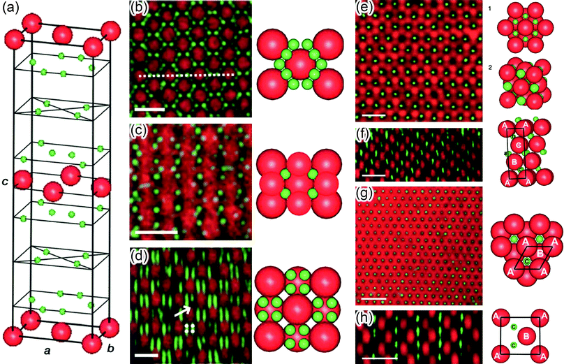 | ||
| Fig. 23 (a–d) AB6-type binary crystals. Positive (green, radius 0.36 μm) and negative (red, 1.16 μm) PMMA-particles in TBAB-containing CHB-decalin, forming a structure with AB6 stoichiometry. (a) Unit cell and (b–d) confocal images and models of different ab-projections. The arrow indicates a “missing” particle. All scale bars are 4 μm. (e–h) AB-type binary crystals. Charged (red, radius 1.16 μm) and uncharged (green, 0.36 μm) PMMA-particles in CHB-decalin. Confocal images of (e, f)NaCl-type- and (g, h) NiAs-type crystal. Reprinted by permission from Macmillian Publishers Ltd: Nature, 2003.30 | ||
We note that charged colloids offer some practical advantages over small, charged nanoparticles. For one, these particles can be made very monodisperse facilitating crystallization. They can be manipulated with optical tweezers234 and can be arranged in desired patterns or structures with which to study epitaxial growth of colloidal crystals.235,236 Also, they can be imaged by various microscopic modalities including confocal microscopy allowing for the direct reconstruction of the crystal's internal structure.
5. Conclusions and outlook
In summary, it is our hope that the examples presented in this Review, both theoretical and experimental, illustrate the versatility of electrostatic forces in controlling aggregation and self-assembly of nanoscale structures. While a significant amount of fundamental work has been done to quantify electrostatic interactions, the nanoscale still remains a relatively unexplored region where discoveries await. The role of nanoscience is to apply known forces in the design of new nanomaterials, but unfortunately, because of the complexities unique to this size regime, most theoretical justifications come a posteriori. This does not necessarily arise due to the inaccuracy or computational limitations of nano-electrostatic models (although this field continues to develop and improve), but rather to the large disconnect which often exists between those who develop the theory and those who perform the experiments. We hope that, at least in part, this Review will serve as a primer for experimentalists curious about the fundamentals of nanoscale electrostatics and for theorists curious about experimental practice. The rational engineering of nanoscale assembliesvia electrostatic interactions is only possible when these two perspectives work closely together and support one another.Acknowledgements
We acknowledge the assistance of Paul J. Wesson for his contributions to the discussion of continuum models, boundary conditions, and energies of interactions. This work was in part supported by the Materials Research Science and Engineering Center (MRSEC) funded by the National Science Foundation under NSF Award Number DMR-0520513 (D.A.W., and M.O.C). The work was also supported by the Non-equilibrium Energy Research Center (NERC) which is an Energy Frontier Research Center funded by the U.S. Department of Energy, Office of Science, Office of Basic Energy Sciences under Award Number DE-SC0000989 (B.K., and B.A.G.).References
- M. C. Daniel and D. Astruc, Chem. Rev., 2004, 104, 293–346 CrossRef CAS.
- T. S. Ahmadi, Z. L. Wang, T. C. Green, A. Henglein and M. A. El-Sayed, Science, 1996, 272, 1924–1926 CrossRef CAS.
- S. H. Sun, C. B. Murray, D. Weller, L. Folks and A. Moser, Science, 2000, 287, 1989–1992 CrossRef CAS.
- Y. G. Sun and Y. N. Xia, Science, 2002, 298, 2176–2179 CrossRef CAS.
- R. Gref, Y. Minamitake, M. T. Peracchia, V. Trubetskoy, V. Torchilin and R. Langer, Science, 1994, 263, 1600–1603 CrossRef CAS.
- C. R. Martin, Science, 1994, 266, 1961–1966 CrossRef CAS.
- M. Bruchez, M. Moronne, P. Gin, S. Weiss and A. P. Alivisatos, Science, 1998, 281, 2013–2016 CrossRef CAS.
- T. Trindade, P. O'Brien and N. L. Pickett, Chem. Mater., 2001, 13, 3843–3858 CrossRef CAS.
- E. A. Meulenkamp, J. Phys. Chem. B, 1998, 102, 5566–5572 CrossRef CAS.
- S. H. Sun and H. Zeng, J. Am. Chem. Soc., 2002, 124, 8204–8205 CrossRef CAS.
- C. B. Murray, C. R. Kagan and M. G. Bawendi, Annu. Rev. Mater. Sci., 2000, 30, 545–610 CrossRef CAS.
- S. Vaucher, M. Li and S. Mann, Angew. Chem., Int. Ed., 2000, 39, 1793 CrossRef CAS.
- C. Burda, X. B. Chen, R. Narayanan and M. A. El-Sayed, Chem. Rev., 2005, 105, 1025–1102 CrossRef CAS.
- A. N. Shipway, E. Katz and I. Willner, ChemPhysChem, 2000, 1, 18–52 CrossRef CAS.
- A. C. Templeton, M. P. Wuelfing and R. W. Murray, Acc. Chem. Res., 2000, 33, 27–36 CrossRef CAS.
- R. Elghanian, J. J. Storhoff, R. C. Mucic, R. L. Letsinger and C. A. Mirkin, Science, 1997, 277, 1078–1081 CrossRef CAS.
- K. L. Kelly, E. Coronado, L. L. Zhao and G. C. Schatz, J. Phys. Chem. B, 2003, 107, 668–677 CrossRef CAS.
- K. S. Lee and M. A. El-Sayed, J. Phys. Chem. B, 2006, 110, 19220–19225 CrossRef CAS.
- W. P. McConnell, J. P. Novak, L. C. Brousseau, R. R. Fuierer, R. C. Tenent and D. L. Feldheim, J. Phys. Chem. B, 2000, 104, 8925–8930 CrossRef CAS.
- L. J. Sherry, R. C. Jin, C. A. Mirkin, G. C. Schatz and R. P. Van Duyne, Nano Lett., 2006, 6, 2060–2065 CrossRef CAS.
- J. J. Storhoff, A. A. Lazarides, R. C. Mucic, C. A. Mirkin, R. L. Letsinger and G. C. Schatz, J. Am. Chem. Soc., 2000, 122, 4640–4650 CrossRef CAS.
- A. Nitzan and M. A. Ratner, Science, 2003, 300, 1384–1389 CrossRef CAS.
- A. T. Bell, Science, 2003, 299, 1688–1691 CrossRef CAS.
- M. Haruta, Gold Bulletin, 2004, 37, 27–36 CAS.
- R. Narayanan and M. A. El-Sayed, J. Phys. Chem. B, 2005, 109, 12663–12676 CrossRef CAS.
- J. Y. Park, Y. Zhang, M. Grass, T. Zhang and G. A. Somorjai, Nano Lett., 2008, 8, 673–677 CrossRef CAS.
- N. Tian, Z. Y. Zhou, S. G. Sun, Y. Ding and Z. L. Wang, Science, 2007, 316, 732–735 CrossRef CAS.
- A. M. Kalsin, M. Fialkowski, M. Paszewski, S. K. Smoukov, K. J. M. Bishop and B. A. Grzybowski, Science, 2006, 312, 420–424 CrossRef CAS.
- W. Kung, P. Gonzalez-Mozuelos and M. O. de la Cruz, Soft Matter, 2010, 6, 331–341 RSC.
- M. E. Leunissen, C. G. Christova, A. P. Hynninen, C. P. Royall, A. I. Campbell, A. Imhof, M. Dijkstra, R. van Roij and A. van Blaaderen, Nature, 2005, 437, 235–240 CrossRef CAS.
- S. Y. Park, A. K. R. Lytton-Jean, B. Lee, S. Weigand, G. C. Schatz and C. A. Mirkin, Nature, 2008, 451, 553–556 CrossRef CAS.
- E. V. Shevchenko, D. V. Talapin, N. A. Kotov, S. O'Brien and C. B. Murray, Nature, 2006, 439, 55–59 CrossRef.
- Z. Y. Tang, Z. L. Zhang, Y. Wang, S. C. Glotzer and N. A. Kotov, Science, 2006, 314, 274–278 CrossRef CAS.
- I. Hussain, Z. X. Wang, A. I. Cooper and M. Brust, Langmuir, 2006, 22, 2938–2941 CrossRef CAS.
- R. Klajn, K. J. M. Bishop, M. Fialkowski, M. Paszewski, C. J. Campbell, T. P. Gray and B. A. Grzybowski, Science, 2007, 316, 261–264 CrossRef CAS.
- M. M. Maye, J. Luo, I. I. S. Lim, L. Han, N. N. Kariuki, D. Rabinovich, T. B. Liu and C. J. Zhong, J. Am. Chem. Soc., 2003, 125, 9906–9907 CrossRef CAS.
- T. K. Sau and C. J. Murphy, Langmuir, 2005, 21, 2923–2929 CrossRef CAS.
- C. B. Murray, C. R. Kagan and M. G. Bawendi, Science, 1995, 270, 1335–1338 CrossRef CAS.
- N. R. Jana, Angew. Chem., Int. Ed., 2004, 43, 1536–1540 CrossRef CAS.
- S. A. Harfenist, Z. L. Wang, M. M. Alvarez, I. Vezmar and R. L. Whetten, J. Phys. Chem., 1996, 100, 13904–13910 CrossRef CAS.
- B. A. Grzybowski, A. Winkleman, J. A. Wiles, Y. Brumer and G. M. Whitesides, Nat. Mater., 2003, 2, 241–245 CrossRef CAS.
- E. C. Hao, B. Yang, J. H. Zhang, X. Zhang, J. Q. Sun and S. C. Shen, J. Mater. Chem., 1998, 8, 1327–1328 RSC.
- J. Kolny, A. Kornowski and H. Weller, Nano Lett., 2002, 2, 361–364 CrossRef CAS.
- D. Lee, M. F. Rubner and R. E. Cohen, Nano Lett., 2006, 6, 2305–2312 CrossRef CAS.
- A. N. Shipway, M. Lahav, R. Gabai and I. Willner, Langmuir, 2000, 16, 8789–8795 CrossRef CAS.
- D. A. Walker and V. K. Gupta, Nanotechnology, 2008, 19 Search PubMed.
- R. Klajn, K. J. M. Bishop and B. A. Grzybowski, Proc. Natl. Acad. Sci. U. S. A., 2007, 104, 10305–10309 CrossRef CAS.
- Z. H. Sun, W. H. Ni, Z. Yang, X. S. Kou, L. Li and J. F. Wang, Small, 2008, 4, 1287–1292 CrossRef CAS.
- D. Philp and J. F. Stoddart, Angew. Chem., Int. Ed., 1996, 35, 1155–1196.
- C. A. Mirkin, R. L. Letsinger, R. C. Mucic and J. J. Storhoff, Nature, 1996, 382, 607–609 CrossRef CAS.
- J. M. Lehn, Angew. Chem., Int. Ed. Engl., 1990, 29, 1304–1319 CrossRef.
- M. Kimura, S. Kobayashi, T. Kuroda, K. Hanabusa and H. Shirai, Adv. Mater., 2004, 16, 335 CrossRef CAS.
- S. R. Johnson, S. D. Evans and R. Brydson, Langmuir, 1998, 14, 6639–6647 CrossRef CAS.
- X. G. Hu, W. L. Cheng, T. Wang, E. K. Wang and S. J. Dong, Nanotechnology, 2005, 16, 2164–2169 CrossRef CAS.
- L. Cusack, R. Rizza, A. Gorelov and D. Fitzmaurice, Angew. Chem., Int. Ed. Engl., 1997, 36, 848–851 CrossRef CAS.
- A. K. Boal, F. Ilhan, J. E. DeRouchey, T. Thurn-Albrecht, T. P. Russell and V. M. Rotello, Nature, 2000, 404, 746–748 CrossRef CAS.
- A. P. Alivisatos, K. P. Johnsson, X. G. Peng, T. E. Wilson, C. J. Loweth, M. P. Bruchez and P. G. Schultz, Nature, 1996, 382, 609–611 CrossRef CAS.
- Y. H. Wei, R. Klajn, A. O. Pinchuk and B. A. Grzybowski, Small, 2008, 4, 1635–1639 CrossRef CAS.
- M. Golosovsky, Y. Saado and D. Davidov, Appl. Phys. Lett., 1999, 75, 4168–4170 CrossRef CAS.
- S. L. Tripp, S. V. Pusztay, A. E. Ribbe and A. Wei, J. Am. Chem. Soc., 2002, 124, 7914–7915 CrossRef CAS.
- H. Zeng, J. Li, J. P. Liu, Z. L. Wang and S. H. Sun, Nature, 2002, 420, 395–398 CrossRef CAS.
- Y. Sahoo, M. Cheon, S. Wang, H. Luo, E. P. Furlani and P. N. Prasad, J. Phys. Chem. B, 2004, 108, 3380–3383 CrossRef CAS.
- B. Kowalczyk, A. M. Kalsin, R. Orlik, K. J. M. Bishop, A. Z. Patashinskii, A. Mitus and B. A. Grzybowski, Chem.–Eur. J., 2009, 15, 2032–2035 CrossRef CAS.
- T. Hirakura, Y. Nomura, Y. Aoyama and K. Akiyoshi, Biomacromolecules, 2004, 5, 1804–1809 CrossRef CAS.
- B. I. Ipe, S. Mahima and K. G. Thomas, J. Am. Chem. Soc., 2003, 125, 7174–7175 CrossRef CAS.
- N. Katsonis, M. Lubomska, M. M. Pollard, B. L. Feringa and P. Rudolf, Prog. Surf. Sci., 2007, 82, 407–434 CrossRef CAS.
- T. Vossmeyer, E. DeIonno and J. R. Heath, Angew. Chem., Int. Ed. Engl., 1997, 36, 1080–1083 CrossRef CAS.
- H. Hiramatsu and F. E. Osterloh, Langmuir, 2003, 19, 7003–7011 CrossRef CAS.
- C. J. Orendorff, P. L. Hankins and C. J. Murphy, Langmuir, 2005, 21, 2022–2026 CrossRef CAS.
- S. Cammas, K. Suzuki, C. Sone, Y. Sakurai, K. Kataoka and T. Okano, J. Controlled Release, 1997, 48, 157–164 CrossRef CAS.
- N. N. Guan, J. Xu, L. Y. Wang and D. J. Sun, Colloids Surf., A, 2009, 346, 221–228 CrossRef CAS.
- Y. Lu, G. L. Liu and L. P. Lee, Nano Lett., 2005, 5, 5–9 CrossRef CAS.
- E. C. M. Vermolen, A. Kuijk, L. C. Filion, M. Hermes, J. H. J. Thijssen, M. Dijkstra and A. van Blaaderen, Proc. Natl. Acad. Sci. U. S. A., 2009, 106, 16063–16067 CrossRef CAS.
- C. C. You, M. De, G. Han and V. M. Rotello, J. Am. Chem. Soc., 2005, 127, 12873–12881 CrossRef CAS.
- R. Hong, N. O. Fischer, A. Verma, C. M. Goodman, T. Emrick and V. M. Rotello, J. Am. Chem. Soc., 2004, 126, 739–743 CrossRef CAS.
- S. H. Brewer, W. R. Glomm, M. C. Johnson, M. K. Knag and S. Franzen, Langmuir, 2005, 21, 9303–9307 CrossRef CAS.
- S. Phadtare, V. P. Vinod, K. Mukhopadhyay, A. Kumar, M. Rao, R. V. Chaudhari and M. Sastry, Biotechnol. Bioeng., 2004, 85, 629–637 CrossRef CAS.
- A. Gole, C. Dash, V. Ramakrishnan, S. R. Sainkar, A. B. Mandale, M. Rao and M. Sastry, Langmuir, 2001, 17, 1674–1679 CrossRef CAS.
- P. Asuri, S. S. Karajanagi, A. A. Vertegel, J. S. Dordick and R. S. Kane, J. Nanosci. Nanotechnol., 2007, 7, 1675–1678 CrossRef CAS.
- Y. F. Huang, C. C. Huang and H. T. Chang, Langmuir, 2003, 19, 7498–7502 CrossRef CAS.
- A. Gole, C. Dash, C. Soman, S. R. Sainkar, M. Rao and M. Sastry, Bioconjugate Chem., 2001, 12, 684–690 CrossRef CAS.
- A. Dyal, K. Loos, M. Noto, S. W. Chang, C. Spagnoli, K. Shafi, A. Ulman, M. Cowman and R. A. Gross, J. Am. Chem. Soc., 2003, 125, 1684–1685 CrossRef CAS.
- E. J. Bjerneld, Z. Foldes-Papp, M. Kall and R. Rigler, J. Phys. Chem. B, 2002, 106, 1213–1218 CrossRef CAS.
- M. E. Aubin, D. G. Morales and K. Hamad-Schifferli, Nano Lett., 2005, 5, 519–522 CrossRef CAS.
- L. Wang and E. K. Wang, Electrochem. Commun., 2004, 6, 49–54 CrossRef CAS.
- T. Pascher, J. P. Chesick, J. R. Winkler and H. B. Gray, Science, 1996, 271, 1558–1560 CrossRef CAS.
- H. Q. Liu, Y. Tian and Z. F. Deng, Langmuir, 2007, 23, 9487–9494 CrossRef CAS.
- K. R. Brown, A. P. Fox and M. J. Natan, J. Am. Chem. Soc., 1996, 118, 1154–1157 CrossRef CAS.
- W. J. Parak, T. Pellegrino, C. M. Micheel, D. Gerion, S. C. Williams and A. P. Alivisatos, Nano Lett., 2003, 3, 33–36 CrossRef CAS.
- T. G. Drummond, M. G. Hill and J. K. Barton, Nat. Biotechnol., 2003, 21, 1192–1199 CrossRef CAS.
- C. M. Niemeyer, Angew. Chem., Int. Ed., 2001, 40, 4128–4158 CrossRef CAS.
- N. L. Rosi and C. A. Mirkin, Chem. Rev., 2005, 105, 1547–1562 CrossRef CAS.
- H. X. Li and L. Rothberg, Proc. Natl. Acad. Sci. U. S. A., 2004, 101, 14036–14039 CrossRef CAS.
- M. G. Warner and J. E. Hutchison, Nat. Mater., 2003, 2, 272–277 CrossRef CAS.
- J. L. Coffer, S. R. Bigham, X. Li, R. F. Pinizzotto, Y. G. Rho, R. M. Pirtle and I. L. Pirtle, Appl. Phys. Lett., 1996, 69, 3851–3853 CrossRef CAS.
- J. Wang, R. Polsky, A. Merkoci and K. L. Turner, Langmuir, 2003, 19, 989–991 CrossRef CAS.
- M. Rycenga, J. M. McLellan and Y. Xia, Adv. Mater., 2008, 20, 2416 CrossRef CAS.
- J. Zhou, J. An, B. Tang, S. P. Xu, Y. X. Cao, B. Zhao, W. Q. Xu, J. J. Chang and J. R. Lombardi, Langmuir, 2008, 24, 10407–10413 CrossRef CAS.
- D. A. Walker, C. E. Wilmer, B. Kowalczyk, K. J. M. Bishop and B. A. Grzybowski, Nano Lett., 2010, 10, 2275–2280 CrossRef CAS.
- P. E. Laibinis, G. M. Whitesides, D. L. Allara, Y. T. Tao, A. N. Parikh and R. G. Nuzzo, J. Am. Chem. Soc., 1991, 113, 7152–7167 CrossRef CAS.
- Y. N. Xia and G. M. Whitesides, Annu. Rev. Mater. Sci., 1998, 28, 153–184 CrossRef CAS.
- D. Witt, R. Klajn, P. Barski and B. A. Grzybowski, Curr. Org. Chem., 2004, 8, 1763–1797 CrossRef CAS.
- G. R. Maskaly, R. E. Garcia, W. C. Carter and Y. M. Chiang, Phys. Rev. E: Stat., Nonlinear, Soft Matter Phys., 2006, 73 Search PubMed.
- X. S. Shen, G. Z. Wang, X. Hong and W. Zhu, CrystEngComm, 2009, 11, 753–755 RSC.
- D. A. Walker, K. P. Browne, B. Kowalczyk and B. A. Grzybowski, Angew. Chem., Int. Ed., 2010, 49, 6760–6763 CrossRef CAS.
- C. M. Goodman, C. D. McCusker, T. Yilmaz and V. M. Rotello, Bioconjugate Chem., 2004, 15, 897–900 CrossRef CAS.
- T. R. Pisanic, J. D. Blackwell, V. I. Shubayev, R. R. Finones and S. Jin, Biomaterials, 2007, 28, 2572–2581 CrossRef CAS.
- P. K. Stoimenov, R. L. Klinger, G. L. Marchin and K. J. Klabunde, Langmuir, 2002, 18, 6679–6686 CrossRef CAS.
- T. H. Chung, S. H. Wu, M. Yao, C. W. Lu, Y. S. Lin, Y. Hung, C. Y. Mou, Y. C. Chen and D. M. Huang, Biomaterials, 2007, 28, 2959–2966 CrossRef CAS.
- S. Patil, A. Sandberg, E. Heckert, W. Self and S. Seal, Biomaterials, 2007, 28, 4600–4607 CrossRef CAS.
- C. Wilhelm and F. Gazeau, Biomaterials, 2008, 29, 3161–3174 CrossRef CAS.
- R. G. Nuzzo and D. L. Allara, J. Am. Chem. Soc., 1983, 105, 4481–4483 CrossRef CAS.
- D. L. Allara and R. G. Nuzzo, Langmuir, 1985, 1, 45–52 CrossRef CAS.
- R. Heinz and J. P. Rabe, Langmuir, 1995, 11, 506–511 CrossRef CAS.
- A. Dhirani, M. A. Hines, A. J. Fisher, O. Ismail and P. Guyotsionnest, Langmuir, 1995, 11, 2609–2614 CrossRef CAS.
- A. Nemetz, T. Fischer, A. Ulman and W. Knoll, J. Chem. Phys., 1993, 98, 5912–5919 CrossRef CAS.
- S. M. Driver and D. P. Woodruff, Langmuir, 2000, 16, 6693–6700 CrossRef CAS.
- O. Azzaroni, M. E. Vela, M. Fonticelli, G. Benitez, P. Carro, B. Blum and R. C. Salvarezza, J. Phys. Chem. B, 2003, 107, 13446–13454 CrossRef CAS.
- A. Imanishi, K. Isawa, F. Matsui, T. Tsuduki, T. Yokoyama, H. Kondoh, Y. Kitajima and T. Ohta, Surf. Sci., 1998, 407, 282–292 CrossRef CAS.
- H. Rieley, G. K. Kendall, A. Chan, R. G. Jones, J. Ludecke, D. P. Woodruff and B. C. C. Cowie, Surf. Sci., 1997, 392, 143–152 CrossRef CAS.
- J. A. Williams and C. B. Gorman, J. Phys. Chem. C, 2007, 111, 12804–12810 CrossRef CAS.
- J. C. Love, D. B. Wolfe, R. Haasch, M. L. Chabinyc, K. E. Paul, G. M. Whitesides and R. G. Nuzzo, J. Am. Chem. Soc., 2003, 125, 2597–2609 CrossRef CAS.
- A. Carvalho, M. Geissler, H. Schmid, B. Michel and E. Delamarche, Langmuir, 2002, 18, 2406–2412 CrossRef.
- H. Murayama, N. Ichikuni, Y. Negishi, T. Nagata and T. Tsukuda, Chem. Phys. Lett., 2003, 376, 26–32 CrossRef CAS.
- Z. Mekhalif, J. Riga, J. J. Pireaux and J. Delhalle, Langmuir, 1997, 13, 2285–2290 CrossRef CAS.
- S. Noel, F. Houze, L. Boyer, Z. Mekhalif, J. Delhalle and R. Caudano, IEEE Trans. Compon. Packag. Technol., 1999, 22, 79–84 CrossRef CAS.
- M. E. Castro and J. M. White, Surf. Sci., 1991, 257, 22–32 CrossRef CAS.
- E. Ruckenstein and Z. F. Li, Adv. Colloid Interface Sci., 2005, 113, 43–63 CrossRef CAS.
- D. D. Gandhi, M. Lane, Y. Zhou, A. P. Singh, S. Nayak, U. Tisch, M. Eizenberg and G. Ramanath, Nature, 2007, 447, 299–U292 CrossRef CAS.
- Y. G. Cai, Langmuir, 2009, 25, 5594–5601 CrossRef CAS.
- A. R. Morrill, D. T. Duong, S. J. Lee and M. Moskovits, Chem. Phys. Lett., 2009, 473, 116–119 CrossRef CAS.
- R. Helmy and A. Y. Fadeev, Langmuir, 2002, 18, 8924–8928 CrossRef CAS.
- K. Shafi, A. Ulman, X. Z. Yan, N. L. Yang, M. Himmelhaus and M. Grunze, Langmuir, 2001, 17, 1726–1730 CrossRef CAS.
- M. A. White, J. A. Johnson, J. T. Koberstein and N. J. Turro, J. Am. Chem. Soc., 2006, 128, 11356–11357 CrossRef CAS.
- C. Yee, G. Kataby, A. Ulman, T. Prozorov, H. White, A. King, M. Rafailovich, J. Sokolov and A. Gedanken, Langmuir, 1999, 15, 7111–7115 CrossRef CAS.
- A. K. Gupta and M. Gupta, Biomaterials, 2005, 26, 3995–4021 CrossRef CAS.
- Y. Sahoo, H. Pizem, T. Fried, D. Golodnitsky, L. Burstein, C. N. Sukenik and G. Markovich, Langmuir, 2001, 17, 7907–7911 CrossRef CAS.
- F. Schreiber, Prog. Surf. Sci., 2000, 65, 151–256 CrossRef CAS.
- M. J. Hostetler, J. E. Wingate, C. J. Zhong, J. E. Harris, R. W. Vachet, M. R. Clark, J. D. Londono, S. J. Green, J. J. Stokes, G. D. Wignall, G. L. Glish, M. D. Porter, N. D. Evans and R. W. Murray, Langmuir, 1998, 14, 17–30 CrossRef CAS.
- C. Haensch, S. Hoeppener and U. S. Schubert, Chem. Soc. Rev., 2010, 39, 2323–2334 RSC.
- R. K. Smith, P. A. Lewis and P. S. Weiss, Prog. Surf. Sci., 2004, 75, 1–68 CrossRef CAS.
- J. J. Gooding, F. Mearns, W. R. Yang and J. Q. Liu, Electroanalysis, 2003, 15, 81–96 CrossRef CAS.
- M. O. de la Cruz, Soft Matter, 2008, 4, 1735–1739 RSC.
- H. Helmholtz, Proggendorff's Annals, 1853, 89, 211–233 Search PubMed , 353–377.
- G. Gouy, J. Phys., 1910, 4, 457.
- G. Gouy, Comt. Rend., 1909, 149, 654 Search PubMed.
- D. L. Chapman, Phil. Mag., 1913, 6, 475.
- D. R. Lide, ed., CRC Handbook of Chemistry and Physics, CRC Press, New York, 2005 Search PubMed.
- K. Sharp, A. Jeancharles and B. Honig, J. Phys. Chem., 1992, 96, 3822–3828 CrossRef CAS.
- R. Messina, J. Chem. Phys., 2002, 117, 11062–11074 CrossRef CAS.
- G. I. Guerrero-Garcia, E. Gonzalez-Tovar and M. O. de la Cruz, Soft Matter, 2010, 6, 2056–2065 RSC.
- R. Ramirez and R. Kjellander, J. Chem. Phys., 2003, 119, 11380–11395 CrossRef CAS.
- P. Gonzalez-Mozuelos, M. S. Yeom and M. O. de la Cruz, Eur. Phys. J. E, 2005, 16, 167–178 CrossRef CAS.
- G. I. Guerrero-Garcia, E. Gonzalez-Tovar, M. Lozada-Cassou and F. D. Guevara-Rodriguez, J. Chem. Phys., 2005, 123 Search PubMed.
- G. I. Guerrero-Garcia, E. Gonzalez-Tovar and M. Chavez-Paez, Phys. Rev. E: Stat., Nonlinear, Soft Matter Phys., 2009, 80 Search PubMed.
- F. Jimenez-Angeles and M. Lozoda-Cassou, J. Phys. Chem. B, 2004, 108, 7286–7296 CrossRef CAS.
- M. Quesada-Perez, E. Gonzalez-Tovar, A. Martin-Molina, M. Lozada-Cassou and R. Hidalgo-Alvarez, ChemPhysChem, 2003, 4, 234–248 CrossRef.
- G. I. Guerrero-Garcia, E. Gonzalez-Tovar, M. Chavez-Paez and M. Lozada-Cassou, J. Chem. Phys., 2010, 132 Search PubMed.
- A. P. dos Santos, A. Diehl and Y. Levin, J. Chem. Phys., 2010, 132 Search PubMed.
- A. G. Moreira and R. R. Netz, Phys. Rev. Lett., 2001, 87 Search PubMed.
- A. Naji, S. Jungblut, A. G. Moreira and R. R. Netz, Phys. A, 2005, 352, 131–170 CrossRef.
- J. W. Zwanikken and M. O. de la Cruz, Phys. Rev. E: Stat., Nonlinear, Soft Matter Phys., 2010, 82, 050401 CrossRef.
- This value can also be computed for dipoles and higher order multipoles from changes in the electric field and its derivatives.
- O. Stern, Zeitschrift fur Elektrochemie, 1924, 30, 508–516 CAS.
- A. Travesset and S. Vangaveti, J. Chem. Phys., 2009, 131 Search PubMed.
- H. Trauble and H. Eibl, Proc. Natl. Acad. Sci. U. S. A., 1974, 71, 214–219 CAS.
- D. Y. C. Chan and D. J. Mitchell, J. Colloid Interface Sci., 1983, 95, 193–197 CrossRef CAS.
- A. Coskun, P. J. Wesson, R. Klajn, A. Trabolsi, L. Fang, M. A. Olson, S. K. Dey, B. A. Grzybowski and J. F. Stoddart, J. Am. Chem. Soc., 2010, 132, 4310–4320 CrossRef CAS.
- K. J. M. Bishop, C. E. Wilmer, S. Soh and B. A. Grzybowski, Small, 2009, 5, 1600–1630 CrossRef CAS.
- J. T. G. Overbeek, Colloids Surf., 1990, 51, 61–75 CrossRef CAS.
- B. V. Derjaguin, Kolloid-Z., 1934, 69, 155 CrossRef.
- B. V. Derjaguin, Acta Physico Chimica U.S.S.R., 1939, 10, 333 Search PubMed.
- R. Hogg, T. W. Healy and D. W. Fuerstenau, Trans. Faraday Soc., 1966, 62, 1638 RSC.
- A. B. Glendinning and W. B. Russel, J. Colloid Interface Sci., 1983, 93, 95–104 CrossRef CAS.
- J. W. Krozel and D. A. Saville, J. Colloid Interface Sci., 1992, 150, 365–373 CrossRef CAS.
- S. L. Carnie, D. Y. C. Chan and J. Stankovich, J. Colloid Interface Sci., 1994, 165, 116–128 CrossRef CAS.
- S. L. Carnie, D. Y. C. Chan and J. S. Gunning, Langmuir, 1994, 10, 2993–3009 CrossRef CAS.
- E. J. W. Verwey and J. T. G. Overbeek, Theory of the Stability of Lyophobic Colloids, Elsevier, New York, 1948 Search PubMed.
- J. C. F. Toledano, F. Sciortino and E. Zaccarelli, Soft Matter, 2009, 5, 2390–2398 RSC.
- E. Sanz, K. A. White, P. S. Clegg and M. E. Cates, Phys. Rev. Lett., 2009, 103 Search PubMed.
- M. Brunner, J. Dobnikar, H.-H. von Grunberg and C. Bechinger, Phys. Rev. Lett., 2004, 92, 078301 CrossRef.
- J. Dobnikar, M. Brunner, H. H. von Grunberg and C. Bechinger, Phys. Rev. E: Stat., Nonlinear, Soft Matter Phys., 2004, 69 Search PubMed.
- J. W. Merrill, S. K. Sainis and E. R. Dufresne, Phys. Rev. Lett., 2009, 103, 138301 CrossRef.
- B. V. R. Tata, M. Rajalakshmi and A. K. Arora, Phys. Rev. Lett., 1992, 69, 3778–3781 CrossRef CAS.
- C. Russ, H. H. von Grunberg, M. Dijkstra and R. van Roij, Phys. Rev. E: Stat. Phys., Plasmas, Fluids, Relat. Interdiscip. Top., 2002, 66 Search PubMed.
- A. P. Hynninen, M. Dijkstra and R. van Roij, Phys. Rev. E: Stat., Nonlinear, Soft Matter Phys., 2004, 69 Search PubMed.
- J. Dobnikar, Y. Chen, R. Rzehak and H. H. von Grunberg, J. Phys.: Condens. Matter, 2003, 15, S263–S268 CrossRef CAS.
- G. Vernizzi and M. O. de la Cruz, Proc. Natl. Acad. Sci. U. S. A., 2007, 104, 18382–18386 CrossRef CAS.
- M. J. Stevens, J. Chem. Phys., 2004, 121, 11942–11948 CrossRef CAS.
- K. J. M. Bishop and B. A. Grzybowski, ChemPhysChem, 2007, 8, 2171–2176 CrossRef CAS.
- A. Albert and E. P. Serjeant, Ionization Constants of Acids and Bases, Methuen & Co Ltd., London, 1962 Search PubMed.
- M. Tagliazucchi, M. O. de la Cruz and I. Szleifer, Proc. Natl. Acad. Sci. U. S. A., 2010, 107, 5300–5305 CrossRef CAS.
- P. Gong, J. Genzer and I. Szleifer, Physical Review Letters, 2007, 98 Search PubMed.
- M. A. Carignano and I. Szleifer, J. Chem. Phys., 1993, 98, 5006–5018 CrossRef CAS.
- R. Klajn, L. Fang, A. Coskun, M. A. Olson, P. J. Wesson, J. F. Stoddart and B. A. Grzybowski, J. Am. Chem. Soc., 2009, 131, 4233 CrossRef CAS.
- P. D. Yates, G. V. Franks, S. Biggs and G. J. Jameson, Colloids Surf., A, 2005, 255, 85–90 CrossRef CAS.
- A. Y. Kim and J. C. Berg, J. Colloid Interface Sci., 2000, 229, 607–614 CrossRef CAS.
- J. M. Lopez-Lopez, A. Schmitt, A. Moncho-Jorda and R. Hidalgo-Alvarez, Soft Matter, 2006, 2, 1025–1042 RSC.
- A. O. Pinchuk, A. M. Kalsin, B. Kowalczyk, G. C. Schatz and B. A. Grzybowski, J. Phys. Chem. C, 2007, 111, 11816–11822 CrossRef CAS.
- S. K. Smoukov, K. J. M. Bishop, B. Kowalczyk, A. M. Kalsin and B. A. Grzybowski, J. Am. Chem. Soc., 2007, 129, 15623–15630 CrossRef CAS.
- A. M. Kalsin, A. O. Pinchuk, S. K. Smoukov, M. Paszewski, G. C. Schatz and B. A. Grzybowski, Nano Lett., 2006, 6, 1896–1903 CrossRef CAS.
- A. M. Kalsin, B. Kowalczyk, P. Wesson, M. Paszewski and B. A. Grzybowski, J. Am. Chem. Soc., 2007, 129, 6664 CrossRef CAS.
- A. M. Kalsin, B. Kowalczyk, S. K. Smoukov, R. Klajn and B. A. Grzybowski, J. Am. Chem. Soc., 2006, 128, 15046–15047 CrossRef CAS.
- H. Sellers, A. Ulman, Y. Shnidman and J. E. Eilers, J. Am. Chem. Soc., 1993, 115, 9389–9401 CrossRef CAS.
- B. A. Grzybowski, Chemistry in Motion: Reaction-Diffusion Systems for Micro- and Nanotechnology, John Wiley & Sons Ltd., West Sussex, UK, 2009 Search PubMed.
- Z. Y. Tang, N. A. Kotov and M. Giersig, Science, 2002, 297, 237–240 CrossRef CAS.
- Z. L. Zhang, Z. Y. Tang, N. A. Kotov and S. C. Glotzer, Nano Lett., 2007, 7, 1670–1675 CrossRef CAS.
- S. M. Liff, N. Kumar and G. H. McKinley, Nat. Mater., 2007, 6, 76–83 CrossRef CAS.
- M. Es-Souni and H. Fischer-Brandies, Adv. Funct. Mater., 2008, 18, 3179–3188 CrossRef CAS.
- S. Huda, S. K. Smoukov, H. Nakanishi, B. Kowalczyk, K. Bishop and B. A. Grzybowski, ACS Appl. Mater. Interfaces, 2010, 2, 1206–1210 CrossRef CAS.
- K. V. Tretiakov, K. J. M. Bishop, B. Kowalczyk, A. Jaiswal, M. A. Poggi and B. A. Grzybowski, J. Phys. Chem. A, 2009, 113, 3799–3803 CrossRef CAS.
- M. G. Song, K. J. M. Bishop, A. O. Pinchuk, B. Kowalczyk and B. A. Grzybowski, J. Phys. Chem. C, 2010, 114, 8800–8805 CrossRef CAS.
- L. Filion, M. Marechal, B. van Oorschot, D. Pelt, F. Smallenburg and M. Dijkstra, Physical Review Letters, 2009, 103 Search PubMed.
- V. Sharma, Q. F. Yan, C. C. Wong, W. C. Cartera and Y. M. Chiang, J. Colloid Interface Sci., 2009, 333, 230–236 CrossRef CAS.
- T. Ming, X. S. Kou, H. J. Chen, T. Wang, H. L. Tam, K. W. Cheah, J. Y. Chen and J. F. Wang, Angew. Chem., Int. Ed., 2008, 47, 9685–9690 CrossRef CAS.
- F. Huang, R. Rotstein, S. Fraden, K. E. Kasza and N. T. Flynn, Soft Matter, 2009, 5, 2766–2771 RSC.
- A. Guerrero-Martinez, J. Perez-Juste, E. Carbo-Argibay, G. Tardajos and L. M. Liz-Marzan, Angew. Chem., Int. Ed., 2009, 48, 9484–9488 CrossRef CAS.
- S. C. Glotzer and M. J. Solomon, Nat. Mater., 2007, 6, 557–562 CrossRef.
- R. Boyack and E. C. Le Ru, Phys. Chem. Chem. Phys., 2009, 11, 7398–7405 RSC.
- S. B. Chaney, S. Shanmukh, R. A. Dluhy and Y. P. Zhao, Appl. Phys. Lett., 2005, 87, 3.
- E. Hao and G. C. Schatz, J. Chem. Phys., 2004, 120, 357–366 CrossRef CAS.
- S. M. Nie and S. R. Emery, Science, 1997, 275, 1102–1106 CrossRef CAS.
- B. Nikoobakht, J. P. Wang and M. A. El-Sayed, Chem. Phys. Lett., 2002, 366, 17–23 CrossRef CAS.
- G. B. Irani, T. Huen and F. Wooten, J. Opt. Soc. Am., 1971, 61, 128 CrossRef CAS.
- R. J. Hunter, Foundations of Colloid Science, Oxford University Press, New York, 2001 Search PubMed.
- Our estimates of electrostatic energies neglect edge effects due to finite sizes of the triangles. We note, however, that because of screening, electrostatic forces are relatively-short ranged (∼5 nm), the edge effects are negligible (at most ∼12% of the total electrostatic energy).
- Charge density was calculated from the electrophoretic mobility, as determined by a Malvern Zetasizer Nano-ZS.
- B. Kowalczyk, D. A. Walker, S. Soh and B. A. Grzybowski, Angew. Chem., Int. Ed., 2010, 49, 5737–5741 CrossRef CAS.
- M. C. Roco, in Handbook on Nanoscience, Engineering and Technology, Taylor and Francis, 2 edn, 2007, pp. 3.1-3.26 Search PubMed.
- D. Derks, H. Wisman, A. van Blaaderen and A. Imhof, J. Phys.: Condens. Matter, 2004, 16, S3917–S3927 CrossRef CAS.
- A. Yethiraj and A. van Blaaderen, Nature, 2003, 421, 513–517 CrossRef CAS.
- U. Gasser, E. R. Weeks, A. Schofield, P. N. Pusey and D. A. Weitz, Science, 2001, 292, 258–262 CrossRef CAS.
- E. H. A. de Hoog, W. K. Kegel, A. van Blaaderen and H. N. W. Lekkerkerker, Phys. Rev. E: Stat. Phys., Plasmas, Fluids, Relat. Interdiscip. Top., 2001, 64 Search PubMed.
- J. P. Hoogenboom, D. L. J. Vossen, C. Faivre-Moskalenko, M. Dogterom and A. van Blaaderen, Appl. Phys. Lett., 2002, 80, 4828–4830 CrossRef CAS.
- M. E. Leunissen, H. R. Vutukuri and A. van Blaaderen, Adv. Mater., 2009, 21, 3116 CrossRef CAS.
- A. van der Horst, A. I. Campbell, L. K. van Vugt, D. A. M. Vanmaekelbergh, M. Dogterom and A. van Blaaderen, Opt. Express, 2007, 15, 11629–11639 CrossRef CAS.
- C.-W. Li and B. E. Volcani, Philos. Trans. R. Soc. London, Ser. B, 1984, 304, 519–528 CrossRef.
- K. Y. Win and S. S. Feng, Biomaterials, 2005, 26, 2713–2722 CrossRef CAS.
- B. Honig and A. Nicholls, Science, 1995, 268, 1144–1149 CrossRef CAS.
- G. S. Lee, Y. J. Lee and K. B. Yoon, J. Am. Chem. Soc., 2001, 123, 9769–9779 CrossRef CAS.
- R. C. Mucic, J. J. Storhoff, C. A. Mirkin and R. L. Letsinger, J. Am. Chem. Soc., 1998, 120, 12674–12675 CrossRef CAS.
- E. Dujardin, L. B. Hsin, C. R. C. Wang and S. Mann, Chem. Commun., 2001, 1264–1265 RSC.
- C. Chen, M. C. Daniel, Z. T. Quinkert, M. De, B. Stein, V. D. Bowman, P. R. Chipman, V. M. Rotello, C. C. Kao and B. Dragnea, Nano Lett., 2006, 6, 611–615 CrossRef CAS.
- H. Ohshima and A. Hyono, J. Colloid Interface Sci., 2009, 333, 202–208 CrossRef CAS.
- H. C. Hamaker, Physics, 1937, 4, 1058 Search PubMed.
- J. Mahanty and B. W. Ninham, Dispersion Forces, Academic Press, London, 1976 Search PubMed.
- L. R. White, J. N. Israelachvili and B. W. Ninham, J. Chem. Soc., Faraday Trans. 1, 1976, 72, 2526–2536 RSC.
- D. Wang, R. J. Nap, I. Lagzi, B. Kowalczyk, S. Han, I. Szleifer and B. A. Grzybowski, J. Am. Chem. Soc., 2011 DOI:10.1021/ja108154a.
- A. M. Kalsin and B. A. Grzybowski, Nano Lett., 2007, 7, 1018–1021 CrossRef CAS.
| This journal is © The Royal Society of Chemistry 2011 |